Optical Observations of the Black Hole Candidate XTE J1550-564 During Re-Flare and Quiescence

Abstract

We report optical monitoring of the soft X-ray transient XTE J1550-564 during the 1999 season (4 January 1999 to 24 August 1999). The first optical observations available in 1999 show that the peak “re-flare” brightness had exceeded the peak brightness of the initial optical flare in September 1998 by over half a magnitude. We compare the optical re-flare light curves with the total X-ray flux, the power-law flux and disk flux light curves constructed from the spectral fits to RXTE/PCA data made by Sobczak et al. (1999, 2000). During the first 60 days of the observed optical re-flare, we find no correspondence between the thermal component of the X-rays often associated with a disk and the optical flux – the former remains essentially flat whereas the latter declines exponentially and exhibits three substantial dips. However, the power law flux is anti-correlated with the optical dips, suggesting that the optical flux may by up-scattered into the X-ray by the hot corona. Periodic modulations were discovered during the final stage of the outburst (May to June), with P=$1.546\pm 0.038$ days, and during quiescence (July and August), with P=$1.540\pm 0.008$ days. The analysis of the combined data set reveals a strong signal for a unique period at P=$1.541\pm 0.009$ days, which we believe to be the orbital period.

1 Introduction

X-ray binaries, which contain a neutron star or a black hole, are among the brightest and most carefully studied X-ray sources. A subclass of X-ray binaries, called soft X-ray transients (SXTs) or X-ray novae, are mass transferring binaries in which the Roche filling mass donor is a dwarf or sub-giant and the accreting compact object is a black hole or a neutron star. SXTs undergo long periods of quiescence (when the X-ray luminosity is $\leq 10^{33}$ergs s^-1) which is occasionally interrupted by luminous X-ray and optical outbursts lasting anywhere from $\sim 10$ to $\gtrsim$ 100 days (Tanaka & Shibazaki 1996; Chen, Shrader, & Livio 1997). The mass function, which is a firm lower limit on the mass of the compact object, can be obtained from optical observations for systems which are bright in quiescence and dominated by the secondary star. The inclination and mass ratio can also be determined, leading to a complete knowledge of the orbital parameters and the masses.

Nine SXTs have been shown to contain a black hole (van Paradijs & McClintock 1995; Bailyn et al. 1998; Orosz et al. 1998a, Filippenko et al. 1999), as their mass functions, or the constrained masses, exceed the maximum stable limit of a neutron star, which is $\approx 3M_{\sun}$ (Chitre & Hartle 1976). In comparison to the numerous observations of SXTs during quiescence (Bradt & McClintock 1983; van Paradijs & McClintock 1995), thorough optical observations of SXTs during outburst are rare. Obtaining good outburst light curves in the optical and in X-ray bands requires an all sky monitor on board an X-ray satellite and uninterrupted access, throughout the year, to an optical telescope. There have been several all sky monitors on previous X-ray satellites, but the opportunity to obtain excellent X-ray light curves of transients dramatically increased with the introduction of the Rossi X-ray Timing Explorer (RXTE). Generally, SXT outbursts are covered with a series of pointed RXTE observations every $\sim$ few days (with energy range between 2-200 keV and time resolution as low as 1$\mu$s), while the All Sky Monitor (ASM; Levine et al. 1996) provides more frequent and less sensitive coverage by scanning most of the X-ray sky every few hours. On the other hand, comparable optical light curves have been difficult to obtain, due to inflexible telescope scheduling, unpredictable weather conditions, and the limitations posed by the position of the object in the night sky. To circumvent the difficulties posed by conventional telescope scheduling, we have used the Yale 1-m telescope located in CTIO and operated by the YALO (Yale, AURA, Lisbon, and Ohio State) consortium. Observations are requested, nightly, via the web and taken by two permanent staff observers, providing the flexible scheduling necessary for studying new outbursts.

Simultaneous X-ray and optical data on SXT outbursts are important for several reasons. First, optical observations provide diagnostics of the properties of the outer accretion disk. The optical emission of a black hole SXT is generally thought to arise in the outer accretion disk due to reprocessing of X-rays that are emitted by the inner disk (van Paradijs & McClintock 1995; King & Ritter 1998). Recent work suggests that the outer disk must be significantly warped in order to explain the high intensity of the reprocessed flux (Esin et al. 1999; hereafter EKMN). A warped disk was also invoked by Esin, Lasota and Hynes (hereafter ELH) to explain the different decay profiles of both optical and X-ray light curves of GRO 1655-40, however the optical light curve was sparsely sampled. In another model for the accretion geometry, the inner accretion disk is replaced by an optically thin ADAF (Narayan, Mahadevan, & Quataert 1998, and references therein). In this case, optical data provide important information required to constrain the spectra predicted by this composite model.

Second, the features of the optical and X-ray light curves are often correlated, with delays spanning several seconds to days. Such delays are related to interesting physical timescales, such as the viscous and thermal timescales or the light-crossing time, which in turn provide information about the $\alpha$-viscosity parameter, radial extent of the disk, and accretion rates. For example, strong evidence in support of the composite ADAF and thin disk model for quiescent SXTs (Lasota 1999) comes from a recent observation of a 6 day delay between the rise of the 1996 optical and X-ray outbursts of GRO 1655-40 (Orosz et al. 1997), which has been successfully modeled by an accretion flow consisting of an outer thin disk and an inner ADAF region (Hameury et al. 1997). However, it is sometimes the case that the X-ray and optical light curves are uncorrelated (e.g. XTE J1550-564, Jain et al. 1999a; this paper). Such contrasting X-ray and optical behavior poses a challenge to models which simply predict an exponentially declining light curve at all wavelengths and to models which simply assume optical photons come from the X-ray heated outer disk.

The soft X-ray transient XTE J1550-564 was discovered with the ASM on the RXTE on September 6, 1998 (Smith et al. 1998). The optical counterpart (Orosz, Bailyn, & Jain 1998b; Jain et al. 1999a) as well as the radio counterpart (Campbell-Wilson et al. 1998) were identified shortly thereafter. Spectra of the optical counterpart during outburst show prominent H$\alpha$ emission as well as broad and weaker emission lines from H$\beta$ and He II (Sánchez-Fernández et al. 1999, hereafter S-F). Based on the equivalent widths of Na D absorption lines and the diffuse interstellar features, S-F find $E(B-V)=0.60$ and infer a distance of 2.5 kpc. The object continued to increase in brightness, reaching a maximum of $6.8$ crab during a bright flare, making XTE J1550-564 the second brightest new X-ray source detected by RXTE (Sobczak et al. 1999).

We have published the X-ray spectral, X-ray timing, and optical results for the period 1998 September 6 to October 28: Sobczak et al. 1999 (Paper I); Remillard et al. 1999 (Paper II); and Jain et al. 1999a (Paper III). We observed the canonical spectral states of a black hole SXT, both the high and low frequency QPOs, and optical responses to large amplitude X-ray fluctuations.

As shown by the ASM X-ray light curve in Fig. 7d, near the end of 1998, the source appeared to be heading towards quiescence (Paper I). However, a prolonged re-flare was observed in the X-ray and optical between MJD 51162 (1998 December 15) and $\sim$ MJD 51350 (1999 June 20). In this paper we report our optical observations and results for this 27 week period. We present comparisons between the optical and X-ray light curves as well as evidence for periodic behavior in the optical light curve both during the final stages of outburst and quiescence. The spectral and timing analysis of the RXTE proportional counter array (PCA) data as well as their correlations for both the 1998 and the 1999 data, up to the end of RXTE Gain Epoch 3 (i.e. before 16:30 (UT) on 1999 March 22) can be found in Paper I, II and Sobczak et al. 2000 (hereafter Paper IV).

In §2 we discuss the observation and data reduction methods. In §3 we present the re-flare light curve and discuss some of its salient features. To facilitate the discussion we divide the re-flare light curves into four intervals. In §4 we describe evidence for periodic behavior of the re-flare light curve shortly before and during quiescence. We also discuss the possible origin of the periodic behavior. In §5, we compare the $B$,V and I light curves with the X-ray light curve. The total X-ray flux can be decomposed into contributions from a disk blackbody component and a power law component (Paper IV) and we compare the behavior of each of these components with the optical light curve. In §6 we provide a discussion which compares the present data set with existing models and in §7 we end with a brief summary.

2 Observations and Reductions

We obtained standard (Johnson) $B$, $V$, and (Kron) $I$ and wide bandpass Johnson $R$ photometry using the Yale 1m telescope at CTIO, which is currently operated by the YALO consortium (Bailyn et al. 2000). Data were acquired using the ANDICAM optical/IR camera which contains a TEK $2048\times 2048$ CCD with $10.2\times 10.2$ arcmin² field of view with a scale of 0.3 arcsec pixel^-1. There are gaps in the light curve in April due to equipment failure caused by a lightening strike, and early July when the IR array was brought into operation. No IR data was obtained for XTE J1550-564.

Paper III reported data between 1998 September 8.99 and October 26.9. Due to observational constraints imposed by the location of the object in the night sky, we were not able to re-embark on our $BVI$ observing campaign until 1999 January 4. After this, at least one exposure was taken per filter for each night the weather and equipment permitted. We concluded the $B$, $V$, and $I$ observations on 1999 May 7.3 as the source brightness approached the limiting magnitudes. During 1999, we obtained 241, 280, and 262 exposures in $B$, $V$, and $I$, respectively, with observation times ranging between 300 and 1200 seconds (see Table 1 for journal of observations).

Although the object was too faint for the $B$, $V$, and $I$ filters by mid-May, we were able to continue observing using the Johnson $R$ (or wide $R$) filter. The bandpass of this filter is approximately the same as the combined bandpass of the standard Kron $R$ and $I$ filters, which makes the wide $R$ filter ideally suited for studying faint red objects. Unfortunately, calibration standards, e.g. those from Landolt, are not available in Johnson $R$ (hereafter simply $R$), therefore we will work exclusively with differential magnitudes. Observations in $R$ started on 1999 April 27 and ended on 1999 August 24. We obtained 171 images with exposure times ranging from 900 to 1200 seconds (see Table 1). The last 82 exposures consist of 41 pairs of 2 consecutive 1200 second integrations, which were summed to increase the signal to noise ratio. The seeing throughout the $B$, $V$, $R$, and $I$ campaign varied from 1.2” to 2.4” with a median value of 1.5”. Ninety percent of the exposures had seeing less than 1.8”.

Preliminary data reduction to make the bias, overscan and flat field corrections, were handled using customized scripts which invoke IRAF routines. The light curve was obtained using IRAF versions of DAOPHOT and the stand-alone code DAOMATCH and DAOMASTER (Stetson 1987, 1992a, 1992b; Stetson, Davis, & Crabtree 1990). The DAOPHOT instrumental magnitudes in $BVI$ were calibrated to standard scales using 4 neighbor stars, whose calibrated magnitudes were obtained previously (see Fig. 7, Table 2 and Paper III)

3 The Re-flare Light Curve

Based on the ASM light curve from late October and November of 1998, XTE J1550-564 appeared to be heading steadily towards quiescence. However, by December 15th, the X-ray flux of the source had clearly increased, as the ASM count rate from this time is double the average count rate of the previous 35 days (see Fig. 7d). This was the beginning of a X-ray re-flare which eventually lasted for $\sim 140$ days. The optical monitoring did not cover the earliest stages of the re-flare, and by the time we resumed observations in early January, the source had brightened by 0.54, 0.8, and 0.60 magnitudes in $B$, $V$, and $I$, respectively, compared to the values obtained during the optical flare in September 1998 (see Fig 7, Paper III).

The general features of the light curve of the 1999 re-flare data differ substantially from the 1998 light curve (Paper III). With the exception of one large flare, the 1998 optical light curves can be described as an exponential decay of the flux with constant e-folding timescale of $\sim 30$ days. Low amplitude flares, dips, and periodic signals in the light curve were generally not observed. Slight deviations from the smooth exponential decline can be found during the first ten and the last seven days of the 1998 light curve, which can better be described as plateau periods. On the other hand, the re-flare light curve exhibited a wider range of phenomena. In Fig. 7 we have plotted the $V$, $V-I$, $R$, ASM count rate and ASM hardness ratio (HR2) light curves (where HR2 is defined as the ratio of 5-12 counts and 3-5 keV counts). The $R$ light curve was placed on the same scale as the $V$ light curve by adding an offset determined from the data taken in late April when both filters were used. This was done only to facilitate the comparison of the $R$ light curve with other colors, and these magnitudes should not be taken to represent true $R$ magnitudes since $V-R$, presumably, is not zero. To draw attention to the salient features of the light curve, we have divided the observation run into four intervals (with days in units of MJD): Interval 1 (51180 to 51229), Interval 2 (51230 to 51313), Interval 3 (51314 to 51345), and Interval 4 (51346 to 51420) – see Table 3 & Fig. 7.

3.1 Interval 1 – Large Flux and Slow Decay

During Interval 1 the optical brightness decreased very slowly, and roughly exponentially at a rate of $\sim$0.009 mag/day in $V$, corresponding to an e-folding time of 121 days (see Figs. 7, 7, and 7). During this time, there were two sharp dips in the optical light curve, which occurred around MJD 51200 and 51215 with amplitudes of $\sim 0.33$ and 0.25 in $B$, $\sim$0.32 and 0.25 in $V$, and $\sim 0.32$ and 0.24 in $I$ (see Figs. 7 and 7). Each of the dips lasted $\sim 3$ days. Other than these two features, the light curve does not deviate significantly from an exponential decay. The $V-I$ color increased slowly at a rate of about $6\times 10^{-4}$ magnitudes/day, which corresponds to a slight reddening of the system. We do not find periodic signatures from the de-trended data from Interval 1.

3.2 Interval 2 – Steep Decline with Random Variability

Around MJD 51231, the optical flux of XTE J1550-564 began to drop dramatically and deviate strongly from the smooth exponential decline found during Interval 1 (see Figs. 7 & 7). Within the first three days of Interval 2, between MJD 51230.34 and 51233.40, the $V$-band flux dropped by $\sim$0.6 magnitudes, nearly 22 times more rapidly than the rate found during Interval 1. Subsequently, the source brightened by $\sim 0.21$ mag in the next 5 days (or by MJD 51238.27) and then decreased again in brightness by $\sim 0.85$ magnitudes during the next 4 days. Between MJD 51244 and 51300 the optical light curve is much less variable and resembles an exponential decline with an e-folding time of $\sim 27$ days, or a decay of $\sim 0.04$ mag/day, which is $\sim 5$ times larger than the value found during Interval 1. There is also flickering in the light curve, of order $0.1\sim 0.2$ magnitudes superposed on this decaying component. As mentioned in section II, there is a substantial gap in the light curves between MJD 51267 and 51294; however it is likely that the $V$ light curve during the gap continued with the exponential decline, as the data immediately after the gap are still consistent with the exponential decay. Finally, the $V$ light curve tapers into a brief plateau as the rate of decay between MJD 51300 and 51313 diminishes to $\sim 1.4\times 10^{-3}$ mag/day, corresponding to an e-folding time of $\sim 776$ days.

We began our $R$-band observations on MJD 51295.18 (see Fig. 7). The $R$-band data is essentially flat between MJD 51295 and 51312 with minimal decay of only $\sim 3.1\times 10^{-3}$ mags/day. It is difficult to compare the $R$ light curve to the $V$ light curve due to the small number of data points which overlap in time. However, the transition from an exponential decay to a plateau which is seen in the $V$ light curve during the last few days of Interval 2, just before MJD $\sim 51300$, is difficult to see in the $R$ light curve (Fig. 7 & 7). It may be that this transition occurred earlier in $R$, prior to our first observations in this filter.

3.3 Interval 3 – Exponential Decay with Periodic Variability

During Interval 3 (between MJD 51313 and 51345) and the next interval, data were collected only in $R$ as the object was too faint for the narrower $V$ and $I$ filters. Contrary to the indications near the end of Interval 2 that the source might be approaching quiescence, its brightness continued to decline throughout Interval 3 (see Figs. 7 and 7). We find no dips of the sort found in Intervals 1 and 2. The light curve can be described as a superposition of a sinusoidal component and an exponential decay, with a rate of $\sim 0.048$ mags/day or e-folding time of $\sim 22.6$ days. This value is comparable to the e-folding time of $\sim 27$ days found during the exponentially decaying phase of Interval 2. Detailed discussion of the periodic component of the light curve during this interval follows in section 4.

3.4 Interval 4 – Quiescence

Between MJD 51346 and the end of the observing campaign on MJD 51420, we believe the source was in or close to full quiescence. A linear fit to the light curve reveals a slight decreasing trend in the brightness, with a rate of $\sim 3.0\times 10^{-3}$ mag/day or an e-folding time of 362 days (see Fig. 7 &7). As there was still a decaying component to the light curve, there remains the possibility that true quiescence had not been reached. During Interval 4, the source brightness was approaching the limiting magnitude of the instrument, hence we averaged two consecutive 1200s integrations to increase the signal to noise ratio. In addition, due to inclement weather and engineering tests, we were unable to get data on a daily basis, with notable gaps between MJD 51368 and 51378 and MJD 51395 and 51406, thus limiting our analysis.

It is important to establish the quiescent magnitude corresponding to a standard set of filters to facilitate comparisons with other sources. Unfortunately the quiescent data were taken using the wide-$R$ filter, which is difficult to calibrate using conventional methods (e.g. via Landolt standards). However, during the last ten days of Interval 2, the light curve is relatively flat, and moreover we have data available in all four filters. Assuming the source did not change color significantly, we can estimate the $B$, $V$, and $I$ magnitudes in quiescence by adding the difference between the average $R$ band magnitudes from the end of Interval 2 and 4 to the $B$, $V$, and $I$ magnitudes from the end of Interval 2. Clearly, the assumption of constant color may be wrong as the $V-I$ color changed substantially, during the steep decline of Interval 2 (see Figure 7). If we adopt the change in $V-I$ color observed during Interval 2, $\sim 0.34$ mags as an additional source of uncertainty, we obtain the mean quiescent $V$ and $I$ magnitudes of $21.3\pm 0.4$ and $19.01\pm 0.4$, respectively. This value is similar to that of XN Oph 1977 which has a quiescent $m_{V}=21.3$ (Remillard et al. 1996). There are only four data points in the $B$-band data during the last ten days of Interval 2 and the associated errors are large due to the faintness of the source. Hence the quiescent $B$ value of $22.7\pm 0.4$ must be taken with some caution. However, this value is consistent with the quiescent magnitude of $22\pm 0.5$ which was obtained from aperture photometry of the digitized SERC J plate No. J2977 (Paper III).

4 Timing Analysis of Intervals 3 and 4

We find strong evidence for periodic signatures from Intervals 3 (Jain et al. 1999b) and 4. Before applying the period searching algorithms, the data had to be de-trended in order to minimize the contribution to the power spectrum from the decaying component of the light curve. The decaying component is subtracted by a linear fit for the data from Interval 3. During interval 4 there is a large gap in the data which roughly separates the light curves into two shorter segments. We took account of the decaying component during Interval 4 by subtracting a linear fit to the entire Interval 4 data set as well as by scaling the average value of the data from both segments to a common value. Subsequently, we used the publicly available time series analysis package PERIOD, which is distributed by project Starlink, to search for periodic signatures in the time series data. Among the various methods for detecting periodic signatures from time series data, we used three independent methods: the CLEAN algorithm (Roberts, Lehár, & Dreher 1987), the Lomb-Scargle periodogram (L-S, Lomb 1976; Scargle 1982; Press & Rybicki 1989), and the phase dispersion minimization algorithm (PDM, Stellingwerf 1978). By using three independent methods, we are less likely to be misled by spurious results.

Using these techniques we have searched for periodic signatures from Intervals 1 through 4. We find no significant peaks in the spectra computed from the de-trended data from Interval 1 and 2. In Fig. 7 we have plotted the results of our period search from Interval 3. We find clear peaks detected by all three methods at $0.647\pm 0.015$ cycles/day corresponding to a period of $1.546\pm 0.038$ days. The quoted uncertainty in the frequency is the half width at half maximum (HWHM) of the gaussian fit to the peaks in the power spectra. We also find weaker peaks corresponding to approximately twice the period. In Fig. 7 we present light curves folded on the three biggest peaks. The light curve folded with a period of $1.546$ days looks the cleanest, although the light curve folded by $3.095\pm 0.044$ days, which is almost exactly double 1.546 days, looks reasonably clean as well. The peak-to-peak amplitude is roughly 0.15 mag although there is substantial scatter, especially at the maximum.

The timing analysis of the data from Interval 4 also provides strong evidence for periodic behavior (see Fig. 7). The analyses show four strong features at $0.296\pm 0.007$, $0.649\pm 0.0032$, $0.652\pm 0.006$, and $1.298\pm 0.006$ cycles/day, corresponding to periods of $3.370\pm 0.076$, $1.540\pm 0.008$, $1.533\pm 0.012$, and $0.770\pm 0.0034$ days, respectively. Here also, the strongest signal is found at $\sim 0.65$ cycles/day. The $R$ band light curve from Interval 4 was folded using the four periods mentioned above. All of the folded light curves look reasonably clean (see Fig. 7), but the cleanest light curve is again obtained by folding with a period of 1.540 days. This folded light curve clearly exhibits two maxima and minima per phase, and the peak-to-peak amplitude is $\sim 0.36$ mags, more than double the value corresponding to Interval 3.

The periodic behavior could be due to several different underlying mechanisms. During outbursts, modulations in the light curve can arise from the precession of the tidally distorted accretion disk, known as superhumps (Whitehurst 1988), or from the X-ray heated secondary star (van Paradijs & McClintock, 1995). During quiescence, if the light curve has periodic features, it is usually an ellipsoidal variation. Ellipsoidal light curves exhibit two equal maxima and two unequal minima when folded by the orbital period (van Paradijs & McClintock 1995). During the transition from outburst to quiescence optical modulations can be caused by a combination of all of these effects.

The presence of disk heating can explain the absence of a second minimum in the folded light curve from Interval 3 (see Fig. 7). As the source was still in outburst during this time, secondary heating from the disk may have been significant enough to produce a broad maximum during superior conjunction, which results in a light curve with only one minimum and one maximum per orbit (Orosz 1996). This scenario is supported by the fact that the peak to peak amplitudes of the optical light curve increased, by a factor of $\sim 2$, as the overall brightness continued to drop between Interval 3 and 4. This can only happen if the modulation was coming from the secondary star and not from the disk itself. Therefore, we favor the interpretation of the Interval 3 and 4 light curves as a combination of secondary heating and ellipsoidal modulation, which together suggest an orbital period $\sim 1.54$ days.

An alternative interpretation of Interval 3 data using superhumps seems to be ruled out by our observations. Superhump periods are usually $\sim 1\%$ longer than the orbital period, hence the combined, detrended Interval 3 and 4 light curves should manifest a phase offset when folded by the the same period, if the Interval 3 periodicity was from a superhump. To test this possibility, we combined the de-trended data from Interval 3 and 4 and performed timing analysis of this joint data set and found a strong peak at $P=1.541\pm 0.009$ days, or frequency of $0.649\pm 0.004$ cycles/day (Fig. 7). The combined data set was folded with 1.541 days and is shown in Fig. 7. As the maxima and minima line up in phase, superhumps appear to be ruled out because a $1\%$ difference in period would have caused an appreciable offset in phase over the span of the observation. The existing evidence shows that the true orbital period is close to 1.54 days and that ellipsoidal variability is present.

5 Correlation with the X-ray Light Curve

During the entire outburst, RXTE PCA and ASM observations were conducted on a daily basis. The detailed analysis of the timing and spectral analysis are presented elsewhere (see Paper I,II,IV). Here we compare the optical light curve from 1998, as well as from Interval 1 and 2 with the X-ray light curve. In particular, we will make use of the detailed spectral information from the PCA data to decompose the total X-ray flux from 2-20 keV into the contribution from the model components. The model used in Papers I and IV consists of the following components: interstellar absorption, multi-color disk blackbody, power law, and a broad Fe emission line. Therefore, based on the fit using the model above, the total X-ray flux can be decomposed into the disk blackbody flux and the power law flux.

From Figs. 7 and 7 it is clear that the shape of the optical and X-ray light curves are quite different. For example, during the steep decline of the 1998 optical light curves between MJD 51080 and 51100, the X-ray disk flux was nearly constant, until MJD 51100 (see Fig. 7) when it suddenly increased. During this time the power law flux decreased very slowly with an e-folding time of $\sim 63.0$ days, nearly double the optical value. The slow decline in the X-ray intensity is unusual, since typically the X-ray decay is much faster than the optical – compare the average e-folding decay time-scales of 17.4 and 67.6 days for the X-ray and optical light curves, respectively, computed from a large sample of SXTs (Chen et al. 1997).

During Interval 1, the earliest stages of the re-flare, the optical flux slowly declined as the X-ray flux first increased slightly and then decreased by a similar amount, thereby producing a concave X-ray light curve with a maximum at around MJD 51200. During Interval 1 there were two prominent dips in the $V$ light curve at MJD 51200.3 and 51215, with amplitudes of $\sim$0.32 & 0.25 respectively (see the Observations section). The disk flux light curve shows no sign of similar dips (see Fig. 7). On the other hand, the power-law flux is anti-correlated with the first optical dip, exhibiting a mini-flare, although there is no response to the second optical dip. The power-law mini-flare peaks at MJD 51201.78, which is nearly 2 days after the peak of the optical dip, and has an X-ray flux of roughly $1.0\times 10^{-8}$ erg s^-1 cm^-2 relative to the ten day average between MJD 51190 and 51200. The relative amplitude of the power-law mini-flare is roughly twice as large as the corresponding optical dip. Since we only have two data points representing this mini-flare, the estimate of the peak could be off by as much as half a day.

At the beginning of Interval 2, MJD 51230, the optical light curve decreases sharply, by $\sim 0.6$ magnitudes. Again, the disk flux showed no change as the optical flux dipped. However, the power-law flux light curve is once again anti-correlated with the $V$-light curve. It is difficult to determine when exactly the power-law flux began to increase, due to the large error bars and sparse data coverage. Clearly, by MJD 51232.25, the power-law flux had increased by $4.42\times 10^{-9}$ erg s^-1 cm^-2, compared to the average values between MJD 51226 to 51230. Since the optical flux during outburst is typically believed to be dominated by the component from the accretion disk, the absence of any correlation between the optical flux and the X-ray disk flux is surprising. On the other hand, our results suggest that both the optical and the power-law component may be a manifestation of the same physical process.

One possibility is that the optical flux is upscattered to the X-ray by the hot corona. In this scenario, during the optical dip, a larger fraction of the optical photons are reprocessed into hard X-rays by compton scattering in the corona, resulting in a decrease in the optical photons accompanied by an increase in the power-law component. This can occur if there is an increase in the size of the corona or an increase in the solid angle it subtends at the outer edge of the disk, or if the opacity suddenly increases. If variations in the properties of the outer edge of the accretion disk were causing the optical dips (e.g. due to a mass transfer instability), we should expect to see a corresponding dip in the X-ray as well, with a delay set by the viscous timescale. The viscous timescale is much longer than the $\sim 2.25$ days delay we find, hence this possibility seems to be ruled out by the data. Nevertheless, even if the optical flux is up-scattered to X-ray, the delay of $\sim 2$ days is difficult to explain since the corresponding light travel time far exceeds the size of the compton cloud. Perhaps there is a time dependence in the efficiency of the scattering resulting in the delay, but it is unclear how this may arise.

Finally, we see remarkable transitions in both the disk flux and power-law light curves starting at around MJD 51240 (see Fig 7). During the next ten days, the disk component dropped by $3.5\times 10^{-8}$ erg s^-1 cm^-2, or by a factor of 3.0 and the power-law flux increased by nearly $3.80\times 10^{-8}$ erg s^-1 cm^-2, or a factor of 4.9. As mentioned before, between MJD 51230 and MJD 51245 there are large fluctuations in the optical light curve, complicating the comparison of the X-ray and optical light curves. Clearly the e-folding timescale of the optical light curves between Interval 1 and 2 are different, but it is not clear whether the transition occurred at around MJD 51230 or MJD 51240 (see Fig. 7). It is clear, however, that the disk flux between MJD 51240 and 51250 is now correlated with the optical whereas the power-law component is anti-correlated. The correlation of the disk flux and anti-correlation of the power-law component with optical magnitudes between MJD 51240 and 51250 suggests the onset of a global change in the accretion disk spanning the outer and inner disk as well as the corona.

6 Discussion

Recent progress has been made in understanding the optical light curve and their relation to the X-ray light curve for a number of well known black hole SXTs. By using a model consisting of an inner ADAF region and an irradiated outer thin disk, Esin et al. have fitted the optical and X-ray light curves of A0620-00, a canonical black hole SXT, and GRS 1124-68, also known as Nova Muscae (see Esin et al. 1997; hereafter EMN, and EKMN). The model essentially depends only on two key parameters, the accretion rate in Eddington units, $\dot{m}$, and the transition radius between the ADAF and the thin disk, $r_{tr}$. The optical flux, which originates from the outer region, is dominated by X-ray irradiation of the disk surface, and therefore is proportional to the X-ray flux emitted from the inner regions (van Paradijs 1996; King & Ritter 1998). It is clear that the particular choice of $\dot{m}$ and $r_{tr}$ will dictate not only the X-ray spectrum but the optical spectrum as well, due to the coupling by X-ray heating. According to the scenario outlined in EMN and EKMN, after the source has reached its maximum brightness, the accretion rate $\dot{m}$ begins to decrease exponentially in time as the transition radius $r_{tr}$ increases, although not necessarily at the same time. At the highest accretion rate and smallest transition radius, the source is in the very high state. Subsequently, as $\dot{m}$ decreases, the source passes through the high state and at a critical value of at $\dot{m}$, reaches the intermediate state when the inner disk starts to evaporate. During the intermediate state, the spectral and temporal characteristics shift from the high state to the low state. Finally, the outer accretion disk is restricted to large radii and the source enters the quiescent state. Spectral transitions, as described above, occurred in XTE J1550-564 throughout the outburst and re-flare (Paper IV; Fig 7). From the very beginning of the outburst to MJD 51115, the object was in the very high state. Between MJD 51115 and 51150 the source faded rapidly and entered the high state, although occasionally the source appeared to be in the intermediate state. During most of the the re-flare (after MJD 51150) the source was in the high state although the source briefly entered the very high state after MJD 51230, at which time the power-law flux increased considerably. Finally the spectrum of one of the last few observations resembles the low state (see Fig. 7). The luminosity of the source was consistent with the scenario laid out by EMN, where the very high state is more luminous than the high state which is in turn more luminous than the intermediate state and low state, with the exception of the last few observations which is perhaps too bright to be in the low state.

Although the scenario laid out by EMN and EKMN applies very well to A0620-00 and Nova Muscae, it is rather difficult to understand the light curves of XTE J1550-564 within this framework. The obvious difficulty lies in the dramatically different morphologies of the optical and X-ray light curves. We also find substantial optical emission during Interval 3, even though there is no discernible X-ray emission. Clearly such behavior can not be explained within the context of a simple irradiated disk, as the optical flux is proportional to the X-ray emission in such models (van Paradijs & McClintock 1995; King & Ritter 1998). Moreover, there are substantial features in the optical light curve, such as sudden changes in the e-folding timescale, dips and mini-flares, which are absent in the X-ray light curve.

Recently ELH have modeled the optical, UV, and X-ray light curves of GRO J1655-40 during the 1996 outburst, which are quite similar to the light curves of XTE J1550-564 from Intervals 1 and 2. Both sources exhibit an exponentially declining optical light curve, whereas the X-ray remains constant or increases slightly. Furthermore, both outbursts began as a flat top with a very high state spectra, followed by a re-flare. The model depends on several critical assumptions. First, the mass transfer rate $\dot{M}_{T}$ must be close to the stability limit for an irradiated disk. Second, $\dot{M}_{T}$ needs to be increased above the critical accretion rate by the irradiation of the secondary due to the X-ray emission from the disk. This prevents the X-ray flux from decreasing exponentially. Finally, the warping of the disk required by recent theoretical work for the outer disk to be irradiated (Dubus et al. 1999) must diminish with a characteristic warp damping time-scale $t_{damp}\sim 4\alpha^{2}t_{vis}$ (ELH) which is about 100 days for $\alpha=0.1$, where $t_{vis}$ is the the viscous time-scale and $\alpha$ is the parameter of viscosity (Shakura & Sunyaev 1973). Due to the incomplete optical coverage of GRO J1655-40, the re-flare which occurred $\sim 270$ days after the initial outburst was not considered at all in ELM. Although this scenario may apply to the optical light curves of XTE J1550-564, judging from the similarity of the source and the light curves, the present data set clearly requires a detailed consideration of the re-flare.

There has been great attention paid to the exponential nature of optical and X-ray light curves, perhaps at the expense of recognizing the interesting exceptions. This is not surprising, as optical data coverage is often incomplete and indeed the prominent X-ray light curve morphology for SXTs is the fast rise followed by an exponential decay (or FREDs) (Chen et al. 1997). Disk instability models generally produce such exponentially decaying light curves (Mineshige & Wheeler 1989; Cannizzo, Chen, & Livio 1995; Hameury et al. 1998). The present data of XTE J1550-564 provide a nearly complete picture of the entire optical outburst including the re-flare, and thus pose a qualitatively more complex challenge to models of outburst and decay of SXTs.

7 Summary

We have presented comprehensive optical light curves for XTE J1550-564 from September 1998 to August 1999 and compared them with the X-ray results presented in Papers I, II, and IV. The shape of the optical and X-ray light curves differ substantially from the typical fast rise and exponential decay and the correspondence between the overall optical and X-ray flux levels is poor, although there are several instances of anti-correlation between the optical flux and the hard power law component of the X-ray system. Analysis of the R-band data at and near quiescence reveal strong periodic signatures at $\sim 1.54$ days with peak to peak amplitudes of 0.15-0.36 mags which we interpret as the orbital period. The single hump behavior in the decay toward quiescence may be due to ellipsoidal modulation and X-ray heating, whereas the double humped signal in quiescence is presumably due to ellipsoidal modulation, with marginal irradiation from the disk. However, more data from quiescence will be required to fully resolve the nature of the modulation.

Top to Bottom (a,b,c,d,e): $B$, $V$, $I$, ASM and ASM HR2 light curves covering the entire observation campaign (including what was presented in Paper III). ASM HR2 (hardness ratio 2) is defined as the ratio of ASM count rates between 5-12 and 3-5 keV. HR2 values were not computed beyond day MJD 51,295 since the ASM count rate is too low to obtain meaningful ratios. The calendar dates are indicated on the top of the plot. The corresponding modified Julian date (MJD) is denoted by the first character of the months, i.e. the labels are left justified with respect to the corresponding MJD.

Finding chart of XTE J1550-564 taken with the YALO 1m telescope (V $3\arcmin\times 3\arcmin$). North is to the right and east is to the bottom.

Top to Bottom (a,b,c,d,e): $V$, $V-I$ color, $R$, ASM and ASM HR2 light curves for the 1999 re-flare. The calendar dates are indicated on the top of the plot. The corresponding MJD is denoted by the first character of the months, i.e. the labels are left justified with respect to the corresponding MJD. The light curve is divided into four intervals as indicated.

The $V$ light curve from Interval 1 (MJD 51180 to 51229). Note the prominent dips and the slow decline, with an e-folding time of 124 days.

The V light curve from Interval 2 (MJD 51230 to 51312). The e-folding time for the data from MJD 51244 to 51300 is 27 days.

The $R$ light curve from Interval 3 (MJD 51313 to 51345). We find evidence for periodic behavior from this interval. The e-folding time is 22.6 days.

The $R$ light curve from Interval 4 (MJD 51346 to 51420). We find periodic motion from this interval as well. There is a slowly decaying component to the light curve corresponding to a very long e-folding time of 362 days.

Result of the three different period searching algorithms for Interval 3 data. From top to bottom: PDM (Phase Dispersion Minimization) statistics, CLEAN power spectrum, and Lomb-Scargle power spectrum. The strongest signals is found at $0.647\pm 0.015$ cycles/day or a period of $1.546\pm 0.038$ days. We also find peaks in the PDM power spectrum at $0.323\pm 0.005$ cycles/day and in the Lomb-Scargle periodogram at $0.356\pm 0.015$ cycles/day, corresponding to periods of $3.095\pm 0.044$ and $2.809\pm 0.03$ days.

De-trended folded R-light curves from Int. 3. Top: The folding period is 1.546 days. The folded light curve is clearly periodic and sinusoidal. Middle: The light curve folded with a period of 2.809 days. Bottom: The light curve folded with a period of 3.095 days. This is nearly double the first folding period, hence we see two cycles per phase.

Result of the three different period searching algorithms for Interval 4. From top to bottom PDM: (Phase Dispersion Minimization) statistics, CLEAN power spectrum, and Lomb-Scargle power spectrum. The strong signals are found at $0.296\pm 0.007$, $0.649\pm 0.0032$, $0.652\pm 0.006$, and $1.298\pm 0.006$ cycles/day (corresponding to periods of $3.370\pm 0.076$, $1.540\pm 0.008$, $1.533\pm 0.012$ and $0.770\pm 0.0034$ days).

De-trended folded light curves from Int. 4, folded with periods corresponding to periods of 0.770, 1.533, 1.540, and 3.370 (from top to bottom). The light curve folded at $P=1.540$ days exhibits a double humped sinusoidal behavior, although there is considerable noise.

Result of three different period searching algorithms for the combined the de-trended data from Int. 3 and Int. 4. From top to bottom: PDM (Phase Dispersion Minimization) statistics, CLEAN power spectrum, and Lomb-Scargle power spectrum. The strongest feature is found at $f=0.649$ cycles/day or $P=1.541$ days.

De-trended folded $R$ light curve from Interval 3 and Interval 4 ($P=1.541$ days). Data from Intervals 3 and 4 were separately de-trended. Squares correspond to data from Interval 3 and the dots correspond to Interval 4. The phase seems to be maintained throughout both intervals.

$V$ light curve and the logarithm of the X-ray fluxes. The X-ray fluxes (2-20keV) are computed from the best fitting model (see Paper I & IV). From top to bottom: The $V$ band light curve, the total X-ray flux, disk flux, and the power law flux light curves. The vertical lines enclose regions with different spectral states, which are indicated in the lowest panel. The source was in the very high state (VHS) from the beginning of the outburst until MJD 51115. Subsequently between MJD 51115 and 51150, the source entered the high state (HS), although occasionally the source appeared to be in the intermediate state (IS). During most of the re-flare (after MJD 51150) the source was in the high state. At the very final stage of the re-flare (beyond MJD 51230) the power-law flux increased and the source temporary entered the very high state before entering the low state (LS).

The same light curves as Fig. 7 zoomed on Intervals 1 & 2. The dashed line corresponds to the optical dip at time 200.3, the dash-dotted line corresponds to the end of Interval 1 and the beginning of Interval 2 and finally the dotted line corresponds to the onset of dramatic global changes in the accretion disk, exemplified by the concurrent changes in the optical flux as well as the disk and power law fluxes.

Table 1: Journal of Observations

	Date MJD, (UT MM/DD)	Number of Exposures	Exposure Times (s)
$B$	$51187.37\sim 51266.27,\ (01/09\sim 03/29)$	230	300, 600, 900
	$51294.37\sim 51304.26,\ (04/26\sim 05/06)$	11	1200s
$V$	$51182.34\sim 51266.25,\ (01/04\sim 03/29)$	260	300, 450
	$51294.36\sim 51312.40,\ (04/26\sim 05/14)$	20	900, 1200
$I$	$51182.35\sim 51266.26,\ (01/04\sim 03/29)$	245	300, 450
	$51294.24\sim 51305.33,\ (04/26\sim 05/07)$	17	900
$R$	$51295.18\sim 51367.16,\ (04/27\sim 07/08)$	136	900, 1200
	$51379.05\sim 51415.00,\ (07/20\sim 08/24)$	34	1200

Table 2: Calibrated Standards

Star ID	$B$	$V$	$I$
A	$18.01\pm 0.03$	$16.13\pm 0.02$	$14.13\pm 0.03$
B	$18.77\pm 0.06$	$16.96\pm 0.02$	$14.89\pm 0.03$
C	$19.11\pm 0.08$	$16.84\pm 0.02$	$14.21\pm 0.03$
D	$15.24\pm 0.02$	$14.48\pm 0.02$	$13.56\pm 0.03$

Table 3: Observation Intervals and the Dates

Interval #	MJD	Periodic	Decay (e-folding timescale)
1	51180-51229	No	124 d
2	51230-51313	No	27 d
3	51314-51345	Yes	22.6 d
4	51346-51420	Yes	362 d

Figure 1:

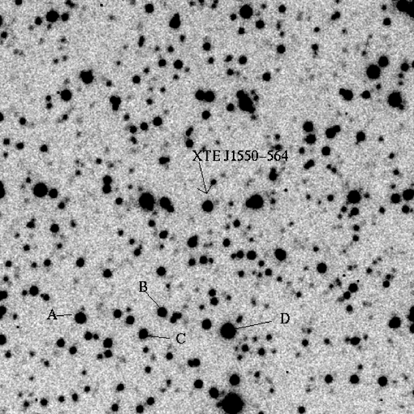
Figure 2:

Figure 3:

Figure 4:

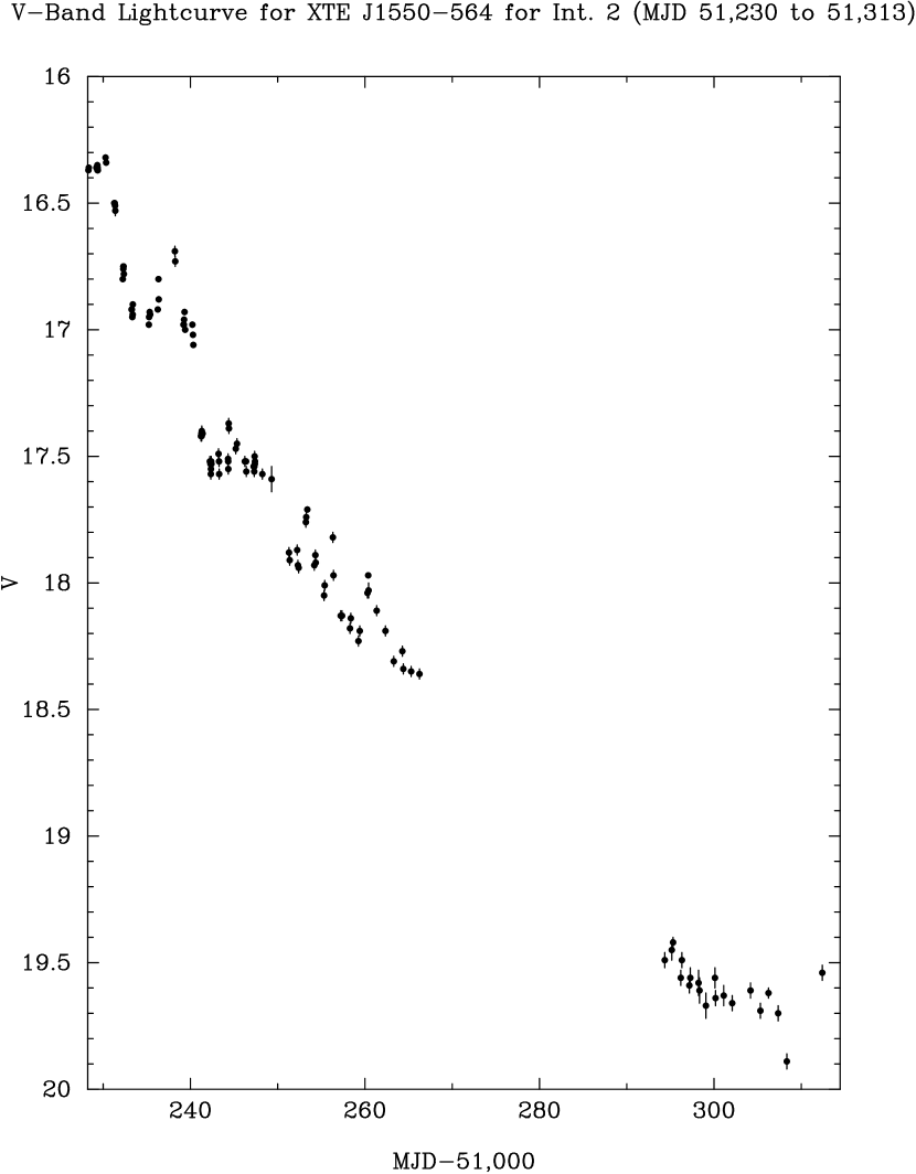
Figure 5:

Figure 6:

Figure 7:

Figure 8:

Figure 9:

Figure 10:

Figure 11:

Figure 12:

Figure 13:

Figure 14:

Figure 15:

References

- (1)
- (2) Bailyn, C. D., Depoy, D., Agostinho, R., Mendez, R., Espinoza, J., & Gonzalez, D. 2000, AAS, 195.8706B
- (3)
- (4) Bailyn, C. D., Jain, R. K., Coppi, P., & Orosz, J. A. 1998, ApJ, 499, 367
- (5)
- (6) Bradt, H. V. D., & McClintock, J. E. 1983, ARA&A, 21, 13
- (7)
- (8) Campbell-Wilson, D., McIntyre, V., Hunstead, R., Green, A., Wilson, R.B., & Wilson, C.A. 1998, IAU Circ., 7010
- (9)
- (10) Cannizzo, J. K., Chen, W., & Livio, M. 1995, ApJ, 454, 880
- (11)
- (12) Chen, W., Shrader, C. R., & Livio, M. 1997, ApJ, 491, 312
- (13)
- (14) Chitre, D. M., & Hartle, J. B. 1976, ApJ, 207, 592
- (15)
- (16) Dubus, G., Lasota, J.-P., Hameury, J.-M., Charles, P. 1999, MNRAS, 303, 139
- (17)
- (18) Esin, A. A., Kuulkers, E., McClintock, J. E., & Narayan, R. 2000, ApJ, 532, 1069 (EKMN)
- (19)
- (20) Esin, A. A., Lasota, J.-P., Hynes, R. I. 2000, A&A, 354, 978 (ELH)
- (21)
- (22) Esin, A. A., McClintock, J. E., Narayan, R. 1997, ApJ, 489, 865 (EMN)
- (23)
- (24) Filippenko et al. 1999, PASP, 111. 969
- (25)
- (26) Hameury, J.-M., Lasota, J.-P., McClintock, J. E., & Narayan, R. 1997, ApJ, 489, 234
- (27)
- (28) Hameury, J.-M., Kristen, M., Dubus, G., Lasota, J.-P., & Hure, J.-M. 1998, MNRAS, 298, 1048
- (29)
- (30) Jain, R. K., Bailyn, C. D., Orosz, J. A., Remillard, R.A., & McClintock, J. E. 1999a, ApJ, 517, L131
- (31)
- (32) Jain, R.K., Bailyn, C. D., Greene, J., Orosz, J. A., Remillard, R.A., & McClintock, J. E. 1999b, IAU Circ., 7187
- (33)
- (34) King, A. R., & Ritter, H. 1998, MNRAS, 293, L42
- (35)
- (36) Landolt, A. U. 1992 AJ, 104, 340
- (37)
- (38) Lasota, J.-P., 1999 in The Theory of Black Hole Accretion Disks, eds. M. A. Abramowicz, G. Björnsson, & J. E. Pringle (Cambridge: Cambridge Univ. Press), 183
- (39)
- (40) Levine, A. M., et al. 1996, ApJ, 469, L33
- (41)
- (42) Lomb, N. R. 1976, Ap&SS, 78, 175
- (43)
- (44) Mineshige, S., & Wheeler, J. C. 1989, ApJ, 343, 241
- (45)
- (46) Narayan, R., Mahadevan, R., & Quataert, E., 1999 in The Theory of Black Hole Accretion Disks, eds. M. A. Abramowicz, G. Björnsson, & J. E. Pringle (Cambridge: Cambridge Univ. Press), 148.
- (47)
- (48) Orosz, J. A., Jain, R. K., Bailyn, C. D., McClintock, J. E., & Remillard, R. A. 1998a, ApJ, 499, 375
- (49)
- (50) Orosz, J. A., Bailyn, C. D., & Jain, R. K. 1998b, IAU Circ., 7009
- (51)
- (52) Orosz, J. A., Remillard, R. A., Bailyn, C. D., McClintock, J. E., 1997, ApJ, 478, L83
- (53)
- (54) Orosz, J. A. 1996, Ph.D. thesis, Yale Univ.
- (55)
- (56) Press, W. H., & Rybicki, G. B. 1989 , ApJ, 338, 277
- (57)
- (58) Remillard, R. A., Orosz, J. A., McClintock, J. E., & Bailyn, C. D. 1996, ApJ, 459, 226
- (59)
- (60) Remillard, R. A., McClintock, J. E., Sobczak, G. J., Bailyn, C. D., Orosz, J. A., Morgan, E. H., & Levine, A. M. 1999, ApJ, 517, L127 (Paper III)
- (61)
- (62) Roberts, D. H., Lehàr, J., & Dreher, J. W. 1987, AJ, 93, 968
- (63)
- (64) Sànchez-Fernàndez 2000, Private Communication
- (65)
- (66) Sànchez-Fernàndez et al. 1999, A&A, 348, L9
- (67)
- (68) Scargle, J. D. 1982, ApJ, 263, 835
- (69)
- (70) Shakura, N. I., & Sunyaev, R. A., 1973, A&A, 24, 337
- (71)
- (72) Smith, D. A., et al. 1998, IAU Circ., 7008
- (73)
- (74) Sobczak, G. J., McClintock, J. E., Remillard, R. A., Cui, W., Levine, A. M., Morgan, E. H., Orosz, J. A. & Bailyn, C. D. 2000, ApJ, 531, 537 (Paper IV)
- (75)
- (76) Sobczak, G. J., McClintock, J. E., Remillard, R. A., Levine, A. M., Morgan, E. H., Bailyn, C. D., & Orosz, J. A. 1999 ApJ, 517, L121 (Paper I)
- (77)
- (78) Stellingwerf, R. F. 1978, ApJ, 224, 953
- (79)
- (80) Stetson, P. B. 1987, PASP, 99, 191
- (81)
- (82) Stetson, P. B., Davis, L. E., & Crabtree, D. R. 1991, in “CCDs in Astronomy,” ed. G. Jacoby, ASP Conference Series, Volume 8, page 282
- (83)
- (84) Stetson, P. B. 1992a, in “Astronomical Data Analysis Software and Systems I,” eds. D. M. Worrall, C. Biemesderfer, & J. Barnes, ASP Conference Series, Volume 25, page 297
- (85)
- (86) Stetson, P. B. 1992b, in “Stellar Photometry—Current Techniques and Future Developments,” IAU Coll. 136, eds. C. J. Butler, & I. Elliot, Cambridge University Press, Cambridge, England, page 291
- (87)
- (88) Tanaka, Y. & Shibazaki, N. 1996, ARA&A, 34, 607
- (89)
- (90) van Paradijs, J., & McClintock, J. E. 1995 in “X-ray Binaries”, eds. W. H. G. Lewin, J. van Paradijs, & E. P. J. van den Heuvel, Cambridge University Press, Cambridge, England, page 58
- (91)
- (92) van Paradijs, J. 1996, ApJ, 464, L139
- (93)
- (94) Whitehurst, R. 1988, MNRAS, 232, 35
- (95)