The Pseudo-$C_{l}$ method: cosmic microwave background anisotropy power spectrum statistics for high precision cosmology

Abstract

As the era of high precision cosmology approaches, the empirically determined power spectrum of the microwave background anisotropy $C_{l}$ will provide a crucial test for cosmological theories. We present an exact semi–analytic framework for the study of the ampling statistics of the $C_{l}$ resulting from observations with partial sky coverage and anisotropic noise distributions. This includes space–borne, air–borne and ground–based experiments. We apply this theory to demonstrate its power for constructing fast but unbiased approximate methods for the joint estimation of cosmological parameters. Further applications, such as a test for possible non–Gaussianity of the underlying theory and a “poor man’s power spectrum estimator” are suggested. An appendix derives recursion relations for the efficient computation of the couplings between spherical harmonics on the cut sky.

I Introduction

During the next few years ground based observations and balloon missions [1] as well as satellite observation [2, 3] promise exquisite determinations of the angular distribution of cosmic microwave background (CMB) anisotropies.

Inflationary cosmogonies, the most popular theories of structure formation, predict a statistically isotropic CMB with Gaussian fluctuations. To linear order in perturbation theory this means that within this class of models all cosmologically relevant information contained in the map of anisotropies is distilled in the angular power spectrum $C_{l}$.

An accurate estimate of these quantities therefore promises to have tremendous impact on our knowledge of the global properties of the universe and the physical processes which lead to the formation of structure[4, 5, 6, 7]. This knowledge is quantified in terms of cosmological parameters such as $\Omega_{tot}$, $\Omega_{b}$, $H_{0}$, etc.

The $C_{l}$ are uniquely defined as rotationally invariant quadratic combinations of the coefficients of an expansion of the anisotropy $\frac{\Delta T}{T}$ in spherical harmonics. Their useful statistical properties rest on the the fact that the spherical harmonics are a complete and orthogonal basis set on the sphere. However, in realistic experiments, only part of the celestial sphere is covered, if only because our CMB sky is obscured by the Milky Way. Also, due the particulars of the observational strategy, non–uniform and possibly correlated noise contaminates the observed signal. In order to interpret past observations and forecast the impact of future observations we need a framework for studying the sampling statistics of the $C_{l}$ for incomplete sky coverage in the presence of non–uniform noise.

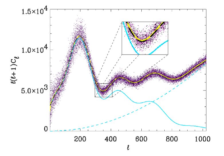
FIG. 1.: The dots are 20 of our 3328 Monte Carlo simulations. On these we superpose the Monte Carlo average (yellow) and the theoretical $C_{l}$ (black dashed), which are the sum of signal (blue, solid) and noise (blue, dashed). The discrepancy seen at low $l$, and to a lesser degree in the inset, demonstrates the effect of correlations due to partial sky coverage even for a satellite experiment capturing 70% of the CMB sky.

It is worth noting that there are several different kinds of $C_{l}$ which we will be referring to in this paper.

The stochastic nature of the observed $C_{l}$ is illustrated in Figure 1, where the straightforward computation of $C_{l}$ from a subset of our Monte Carlo simulations of incomplete and noisy skies are overlaid on the theoretical predictions. One or more of the following simplifying assumptions can be invoked in cases where one would like to avoid the full complexity of the problem (e.g.  [4, 5, 8, 9]):

• (Independence) The observed $C_{l}$ are approximately independent due to nearly full and uniform sky coverage,

• (Scaled $\chi^{2}$) Their sampling distributions do not change appreciably from the $\chi^{2}$ distributions which apply for the full sky, apart from a rescaling of the number of degrees of freedom by the sky fraction $f$, and

• (Gaussianity) Their sampling distributions are well–approximated by Gaussian distributions which have the same first and second moments as these rescaled $\chi^{2}$ distributions.

There are several reasons to carefully assess these approximations and, if necessary, go beyond them. One reason is that in the short term balloon and ground based experiments will provide the leading edge science results to the field. Due to practical limitations we cannot hope to even come close to full sky coverage with these types of experiments. The observation regions are often ring–shaped or cover a circular region of the sky which subtends a small solid angle. It is an urgent matter to assess statistically how these imminent experiments can constrain the power spectrum and cosmological parameters.

Further, the planned satellite missions are aiming to determine the $C_{l}$ to sub–percentage accuracy. In the case of the Planck Surveyor mission, this has given us the hope of detecting small effects such as secondary anisotropies which are due to nonlinear gravitational effects on the CMB photons during the free–streaming epoch. An example of such an effect is anisotropies due to gravitational lensing. This is an important issue because a detection would break otherwise present parameter degeneracies and allow a consistent parameter estimation from CMB data alone [10].

More generally, the impact CMB observations will have on cosmology makes it important to use approximations in a controlled way. For example, in the analysis of COBE–DMR data it was realized that using Gaussian approximations for quadratic quantities introduced systematic biases [11]. At the same time, we need approximations to make feasible the analysis of the huge CMB data sets we expect in the coming years.

The Maximum Likelihood Inversion (MLI) method (cf.  [12, 13, 14, 15] for applications in a cosmological context) is the standard framework for solving this type of problem. To illustrate, we write down the likelihood functional for a Gaussian sky. In order to do so we need to define the vector of observed pixel temperatures on the sky ${\bf{d}}$ with $N_{pix}$ components. A given theory and observational strategy on the sky imply the covariance structure of the elements $d_{i}$ in terms of signal and noise covariance matrices ${\bf{S}}$ and ${\bf{N}}$ such that

$$\left\langle{d_{i}d_{j}}\right\rangle=S_{ij}+N_{ij}.$$ (1)

The signal covariance matrix $S$ is simply a discretised version of the theoretical angular correlation function

$$\xi\!\left(\alpha_{ij}\right)=\sum_{l=2}^{\infty}\frac{2l+1}{4\pi}C_{l}P_{l}(\alpha_{ij}),$$ (2)

evaluated at the pixel locations. The noise covariance ${\bf{N}}$ reflects those imperfections of the experiment and observational strategy which lead to spatial correlations in the projected noise.

This leads to an expression for the likelihood

$$L(d|\mathrm{theory})=\frac{\exp{\left(-{\frac{1}{2}}{\bf{d^{T}}}({\bf{S}}+{\bf{N}})^{-1}{\bf{d}}\right)}}{\sqrt{(2\pi)^{N_{pix}}\left|{{\bf{S}}+{\bf{N}}}\right|}}$$ (3)

The matrix ${\bf{S}}$ is a function of predicted $C_{l}$, which are in turn determined by the parameters of some theory. The matrix ${\bf{N}}$ includes a model of the expected noise covariance given the experimental setup. The structures of both ${\bf{S}}$ and ${\bf{N}}$ also depend on the observed region on the sky.

For a given set of data the likelihood is then considered as a function of the parameters of a given theory. The maximum likelihood parameter estimates are determined as those which maximise Eq. (3). While these manipulations are conceptually simple, the practical difficulties are apparent. The number of operations needed to evaluate Eq. (3) (or equivalently an estimator derived from it) scales as the most costly operations contained in it. These are the determinant evaluation in the denominator and the matrix inverse in the exponent. For a general situation both of these require $N_{pix}^{3}$ operations.

In the near future $N_{pix}$ will be $10^{5}$ from balloon experiments (such as Maxima), then $10^{6}$ for MAP and in less than a decade $10^{7}$–$10^{8}$ for Planck. These numbers imply $10^{15}$–$10^{24}$ computations. Even when considering future growth in computing performance, estimates of the computational time required to evaluate Eq. (3) a single time reach up to many years [16]. To compute the maximum likelihood estimator requires many likelihood evaluations and would thus require an unfeasibly long period of time. For practical purposes, straightforward applications of the MLI method therefore fail to give answers in finite computational time.

Previous studies of this subject have usually directly addressed the problem of ”solving for the $C_{l}$”. Tegmark [17] rejects the maximum likelihood estimator on the grounds that it is too time–consuming to compute and suggests a minimum variance (and hence “optimal”) method based on a quadratic estimator which makes a form of the Gaussianity assumption above. While this method is powerful in the regime where it is applicable, it does not provide a means of assessing the validity of this assumption. Within our analysis we can make the connection between the minimum variance and the maximum likelihood methods (cf.  subsection III A).

The approach of Bond, Jaffe and Knox [18] is again very different from ours. It consists in finding an approximate form for the likelihood and parametrising the shape of the power spectrum in terms of a set of top hat functions, whose height gives the average value of the $C_{l}$ over its width. The width of these top hats is chosen wide enough that correlations between them become small. Their method is of practical significance because their approximate ansatz for the likelihood is easy to evaluate.

Our perspective is the following: we endeavour to provide an ab initio formalism which lays bare the statistical properties of the power spectrum coefficients. It then turns out that the insight gained from this study can be used to formulate unbiased and well–controlled methods for parameter estimation.

FIG. 2.: Annuli, circular patches such as polar caps and even disjoint geometries such as the full sky with an annulus (such as a Galactic cut) removed are within the class for which our formalism is exact.

To provide a quantitative basis for this discussion we present in this paper an efficient semi–analytic calculational framework within which the statistical properties of the $C_{l}$ power spectrum coefficients can be studied for theories which generate a Gaussian CMB sky. This framework is exact for the important class of survey geometries and noise patterns which obey rotational symmetry about one arbitrary axis and is not limited to large sky coverage. This class contains both skies with symmetric and asymmetric cuts north and south of the Galactic equator, rings, annuli, and polar cap shaped regions of any size as indicated in Figure 2. For this class we obtain exact analytical solutions for the mean $\left\langle{C_{l}}\right\rangle$, the variance $\left\langle{\left(\Delta C_{l}\right)^{2}}\right\rangle$, the skewness, kurtosis and all higher moments of the sampling distribution for all $l$. We derive exact and conveniently computable analytic expressions for the marginalised probability distributions of the cut sky $C_{l}$ for all $l$ as well as integral representations for the joint distribution of all $C_{l}$. As an added bonus we find that our methods also allow dealing with arbitrary noise patterns to very good accuracy and conclude by illustrating their use in some applications.

To test our results we perform state–of–the–art Monte Carlo simulations for a high resolution CMB satellite with a Galactic cut of size $\pm 20^{\circ}$ (resulting in a sky coverage comparable to COBE). We use a sine modulated noise template as a simple model of the noise pattern which would result from scanning along great circles through the ecliptic poles. The numerical results we obtain provide a solid check on our analytic calculations.

The plan of this paper is as follows: in section II we lay out the general framework. Section III develops the statistical theory of power spectrum coefficients for observation regions which are azimuthally symmetric about some axis. We arrive at expressions for the cut–sky moments of any order and solve the moment problem to obtain the exact sampling distributions. We compare our analytical results to Monte–Carlo simulations in section IV. Several applications of our methods are presented in section V. Section VI contains further discussion and our conclusions. Appendix A discusses the effects of non-cosmological foregrounds on the results presented in this paper. Details of our analytical and numerical techniques are given in three further appendices.

II The framework

The full sky of CMB temperature fluctuations can be expanded in spherical harmonics, $Y_{lm}$, as

$$T({\bf\gamma})=\sum_{l=0}^{l_{max}}\sum_{m}a_{lm}Y_{lm}(\gamma)$$ (4)

where ${\bf{\gamma}}$ denotes a unit vector pointing at polar angle $\theta$ and azimuth $\phi$. Here we have assumed that there is insignificant signal power in modes with $l>l_{max}$ and introduce the convenient notation that all sums over $m$ run from $-l_{max}$ to $l_{max}$ but all quantities with index ${lm}$ vanish for $m>l$.

In a universe which is globally isotropic and contains Gaussian fluctuations, the $a_{lm}$ are independent, Gaussian distributed with zero mean and specified variance $C^{theory}_{l}\equiv\langle\left|{a_{lm}}\right|^{2}\rangle$. Hence, for noiseless, full sky measurements, each measured $C_{l}$ independently follows a $\chi^{2}$–distribution with $2l+1$ degrees of freedom and mean $C^{theory}$. Owing to Galactic foregrounds, limited surveying time or other constraints inherent in the experimental setup, the temperature map that comes out of an actual measurement will be incomplete. In addition, a given scanning strategy will produce a noise template: high noise per pixel results in regions where the scanning lines are less densely packed compared to regions where they are denser. We model the noise as a Gaussian field with zero mean which is independent from pixel to pixel and modulated by a spatially varying root mean squared amplitude $W_{N}({\bf{\gamma}})*W({\bf{\gamma}})$ (the factor of $W$ appearing because the noise too is zero in unobserved regions). Therefore the observed temperature anisotropy map is in fact

$$\tilde{T}({\bf\gamma})=W({{\bf{\gamma}}})\left[T({{\bf{\gamma}}})+W_{N}({{\bf{\gamma}}})T_{N}({{\bf{\gamma}}})\right]$$ (5)

where $W$ is unity in the observed region and zero elsewhere.

The coefficients in the spherical harmonic expansion recovered from such an incomplete observing region are

$$\tilde{a}_{l^{\prime}m^{\prime}} = \int_{{\cal O}}d\Omega\>Y^{\ast}_{l^{\prime}m^{\prime}}({{\bf{\gamma}}})T({{\bf{\gamma}}})$$ (6)

$$= \sum_{lm}{a_{lm}}\int_{{\cal O}}d\Omega\>Y^{\ast}_{l^{\prime}m^{\prime}}({\bf{\gamma}})Y_{lm}({\bf{\gamma}})$$ (7)

The notation “$\int_{\cal O}$” denotes integration over the observed region. Note that the usual orthogonality property of the $Y_{lm}({\bf{\gamma}})$ does not hold any longer because we do not integrate over all solid angle. This becomes clearer if we define the geometric coupling matrix

$$W_{l^{\prime}m^{\prime}\;lm}\equiv\int_{{\cal O}}d\Omega\>Y^{\ast}_{l^{\prime}m^{\prime}}({\bf{\gamma}})Y_{lm}({\bf{\gamma}})$$ (8)

and write

$$\tilde{a}_{l^{\prime}m^{\prime}}=\sum_{lm}W_{l^{\prime}m^{\prime}\;lm}{a_{lm}}.$$ (9)

By definition, the $W_{l^{\prime}m^{\prime}\;lm}$ are just the matrix elements of the $W({{\bf{\gamma}}})$ window in a spherical harmonic basis. These matrices have been previously discussed in a similar context in the pioneering papers by Peebles and Hauser [19, 20].

This means that expanding $\tilde{T}$ as in Eq. (7) produces a set of correlated Gaussian variates $\tilde{a}_{lm}$ for the signal and $\tilde{a}_{N\;lm}$ for the noise. These combine into power spectrum coefficients

$$\tilde{C}_{l}=\frac{1}{2l+1}\sum_{m}\left|{\tilde{a}_{lm}+\tilde{a}_{N\;lm}}\right|^{2}$$ (10)

whose statistical properties differ from the ones of the $C_{l}$. We therefore refer to these quantities as pseudo-$C_{l}$. In what follows we will discuss the statistical properties of these quantities.

III Exact pseudo–$C_{\l}$ statistics

Let us focus on the terms of the sum Eq. (10). They are squares of Gaussian distributed variates with zero mean. It follows that the $\tilde{C}_{l}$ are sums of $2l+1$ $\chi^{2}$ variates with one degree of freedom. However, each term in the sum has a different expectation value and may in general be correlated, so the $\tilde{C}_{l}$ are not $\chi^{2}$ distributed with 2l+1 degrees of freedom.

If we assume white noise, $C^{N}_{l}\equiv C^{N}$, then each term in the sum has expectation value

$$\sigma^{2}_{lm}=\frac{\sum_{l^{\prime}m^{\prime}}C_{l^{\prime}}\left|{W_{l^{\prime}m^{\prime}\;lm}}\right|^{2}+C^{N}\!\!\int_{O}d{{\bf{\gamma}}}W_{N}({{\bf{\gamma}}})^{2}\lambda^{2}_{lm}(\theta)}{2l+1}$$ (11)

A few remarks are in order:

1. Azimuthal symmetry has not been invoked to derive this relation.

2. The cross–term which comes from expanding the square in Eq. (10) has vanishing expectation value because signal and noise are assumed to be uncorrelated.

3. The sum over $C_{l}$ includes the non–cosmological $l=0$ and $l=1$ terms. The appearance of these terms merits some further discussion, which we relegate to Appendix A.

A Digression: connecting to the least squares estimator

Summing Eq. (11) over $m$ gives a set of linear equations which also results in a different context, namely after minimising the variance of the $C_{l}$ estimator in Tegmark [17]. There it appears as a set of linear equations for the estimator, which the author assumes to be Gaussian distributed.

We see from our treatment that this equation is only valid after the expectation values are taken. The quantities involved are quadratic in Gaussian variates which leads to the presence of a cross term which only disappears after taking the expectation value.

This is the reason why some $C_{l}$ estimates in [17] turn out negative for values of $l$ where the signal to noise ratio becomes of order unity. This is of course unphysical because the $C_{l}$ are properly quadratic and hence positive semi–definite quantities. We observe that it is precisely neglecting this fact which leads to unphysical results.

On the other hand, our treatment provides alternative proof of the fact that the least–squares estimator is unbiased. It also explains the significance of the Fisher matrix which appears in this context: is simply a measure of the geometric couplings between eigenmodes of total angular momentum.

B Azimuthal symmetry

To elucidate the correlation structure between the $\tilde{a}_{lm}$, Eq. (9), we write Eq. (10) as a quadratic form

$$\tilde{C}_{l}=\frac{1}{2l+1}\sum_{m}\>\sum_{l^{\prime},m^{\prime},l^{\prime\prime},m^{\prime\prime}}\xi^{\ast}_{l^{\prime}m^{\prime}}{\cal M}^{(lm)}_{l^{\prime}m^{\prime}l^{\prime\prime}m^{\prime\prime}}\xi_{l^{\prime\prime}m^{\prime\prime}}$$ (12)

in independent normal variates $\xi_{lm}$ with zero mean and unit variance. The object ${\cal M}$ describes the combined effect of statistical correlation and the geometrical couplings between the various expansion coefficients.

For an isotropic Gaussian field on the full sky

$${\cal{M}}^{(lm)}_{l_{1}m_{1}\;l_{2}m_{2}}=\delta_{ll_{1}}\delta_{mm_{1}}\left(C^{theory}_{l}+C^{noise}_{l}\right)\delta_{ll_{2}}\delta_{mm_{2}}.\quad\text{(isotropic, full sky)}$$ (13)

We show in Appendix B that for a Gaussian field with an anisotropic but azimuthally symmetric weight function $W(\theta)$, ${\cal M}$ is of the form

$${\cal{M}}^{(lm)}_{l_{1}m_{1}\;l_{2}m_{2}}=\delta_{mm_{1}}W^{(l)}_{l_{1}m_{1}}\left(C^{theory}_{l}+C^{noise}_{l}\right)W^{(l)}_{l_{2}m_{2}}\delta_{mm_{2}},\quad\text{(anisotropic, cut sky)}$$ (14)

where

$${\cal W}_{l^{\prime}m}^{(l)}\equiv W_{l^{\prime}m\;lm}=\int d\mu W(\mu)\lambda_{lm}(\mu)\lambda_{l^{\prime}m}(\mu),$$ (15)

and we assume identical windows for signal and noise for notational simplicity in Eq. (14). The generalisation for arbitrary azimuthally symmetric noise windows is straightforward.

The structure exhibited in Eqs. (14) and (15) is the key fact which allows the derivation and cheap evaluation of the exact results we obtain. An efficient algorithm for the evaluation of the matrix elements of $W$ is given in appendix C. For a maximum $l$ of 1024 this takes just over one minute on a single R10000 CPU.

It follows that while the $\tilde{a}_{lm}+\tilde{a}_{N\;lm}$ terms in Eq. (10) are correlated for different $l$, they will be independent for different $m$. As a consequence, under the assumption of azimuthal symmetry the $\tilde{C}_{l}$ are sums of independent Chi–squared ($\chi^{2}$) variates, each with one degree of freedom but different expectations. Below we succeed in finding analytical expressions for the probability density functions of such generalised $\chi^{2}$ variates and we hence solve for the statistical properties of the pseudo–$C_{l}$ exactly.

C Pseudo–$C_{\l}$ moments

The problem is to compute the statistical properties of a sum of independent variates, each of which has a known distribution. A useful tool for attacking this kind of problem is the method of characteristic functions [21]. Appendix D provides a heuristic introduction to this method.

The characteristic function of a $\chi^{2}$ variate with one degree of freedom is given by

$$\frac{1}{(1-2ix\sigma_{lm}^{2})^{{\frac{1}{2}}}}.$$ (16)

We can multiply them together for each term in the sum Eq. (10) and inverse Fourier transform to obtain $p(\tilde{C}_{l})$ as

$$p(\tilde{C}_{l})=\frac{1}{2\pi}\int_{-\infty}^{+\infty}dx\frac{e^{-i\tilde{C}_{l}x}}{\prod_{m=-l}^{l}(1-2ix\sigma_{lm}^{2})^{{\frac{1}{2}}}}$$ (17)

The log of the integrand in this expression (not including the complex exponential) is the cumulant generating function, which we can differentiate to obtain all cumulants of the pseudo–$C_{l}$ as

$$\kappa_{n}=2^{n-1}(n-1)!\sum_{m}(\sigma_{lm}^{2})^{n}.$$ (18)

We give the following expressions for the mean, variance, skewness $\beta_{1}=\frac{\langle(\Delta\tilde{C}_{l})^{3}\rangle}{\langle(\Delta\tilde{C}_{l})^{2}\rangle^{\frac{3}{2}}}$ and kurtosis $\beta_{2}=\frac{\langle(\Delta\tilde{C}_{l})^{4}\rangle}{\langle(\Delta\tilde{C}_{l})^{2}\rangle^{2}}$ as examples:

$$\langle\tilde{C}_{l}\rangle=\sum_{m}\sigma^{2}_{lm}$$,

.

(19)

D Pseudo–$C_{\l}$ distributions

It turns out that we do not have to contend with just the cumulants. We will now derive the analytical form for the pseudo–$C_{l}$ distributions. We define $s^{(l)}_{m}=(2/\sigma^{2}_{lm})$ and note that $s^{(l)}_{m}=s^{(l)}_{-m}$. Then all terms with equal $\left|{m}\right|\geq 1$ pair up and we obtain

$$p(\tilde{C}_{l})=\frac{A^{(l)}}{2\pi}\int_{-\infty}^{+\infty}dx\frac{e^{-i\tilde{C}_{l}x}}{(s^{(l)}_{0}-ix)^{{\frac{1}{2}}}\prod_{m=1}^{l}{(s^{(l)}_{m}-ix)}}$$ (20)

where $A^{(l)}\equiv\sqrt{s^{(l)}_{0}}\prod_{m=1}^{l}s^{(l)}_{m}$. We expand in partial fractions and integrate each term analytically (using a standard integral from [22]) to produce a closed form solution in terms of incomplete gamma functions $\gamma(\alpha,x)$:

$$\!\!\!\!\!\!\!\!p(\tilde{C}_{l})={A^{\prime}}^{(l)}\sum_{m=1}^{l}\frac{\exp\left(-s^{(l)}_{m}\tilde{C}_{l}\right)\,\gamma\!\left(\frac{1}{2},(s^{(l)}_{0}-s^{(l)}_{m})\tilde{C}_{l}\right)}{\sqrt{(s^{(l)}_{0}-s^{(l)}_{m})}\prod_{\;m=1}^{{}^{\prime}\;l}(s^{(l)}_{m^{\prime}}-s^{(l)}_{m})}$$ (21)

where the primed product symbol $\prod^{{}^{\prime}}$ only multiplies factors which have $m\neq m^{\prime}$ and the normalization constant is

$${A^{\prime}}^{(l)}\equiv\frac{\sqrt{s^{(l)}_{0}}\prod_{m=1}^{l}s^{(l)}_{m}}{2\Gamma(\frac{3}{2})}.$$ (22)

We have, therefore, reduced the problem of determining the sample probability density of the pseudo–$C_{l}$ to computing the $\sigma_{lm}^{2}$. The computation of these coefficients has to be done only once for a given survey geometry and model theory. In fact it is clear from their definition and Eq. (11) that once the ${\cal W}^{(l)}_{l^{\prime}m}$ are computed for a given survey geometry, the $\sigma_{lm}^{2}$ can be generated very easily given a model $C_{l}$ spectrum.

E Correlations between different $\tilde{C}_{\l}$

The distributions we have just derived are 1-point or marginal distributions. They contain complete statistical information about each $\tilde{C}_{l}$ taken for itself, but they only account for the correlations between $C_{l}$ implicitly, giving an effective distribution for each $\tilde{C}_{l}$ which contains these correlations. To obtain explicit information about the full joint distribution of all $\tilde{C}_{l}$ we must go a step further.

While we wish to relegate further study of the properties of the joint distribution to future work we will now mention some preliminary results.

The characteristic function of the joint distribution of quadratic forms such as Eq. (12) has been studied in the literature [21]. Fourier transforming we can obtain an integral representation of the joint distribution (analogously to Eq. (17) for the 1-point distributions)

$$p\left(\left\{\tilde{C}_{l}\right\}\right)=\frac{1}{(2\pi)^{l_{max}}}\int\frac{\prod_{l}\left(e^{-iS_{l}\tilde{C}_{l}}dS_{l}\right)}{\left|{\openone-2i\sum_{l^{\prime}}S_{l^{\prime}}{\cal M}^{l^{\prime}}}\right|^{{\frac{1}{2}}}}$$ (23)

Even though we cannot proceed further in the Fourier inversion or must take recourse to approximate methods, we can still gain useful information about the joint statistics of the set of $C_{l}$. Similarly to subsection III C we can derive the cumulants of the variates from the logarithm of the integrand (disregarding the complex exponential). It is easy to show that for the covariance between the pseudo–$C_{l}$ we can write

$$\left\langle{\Delta\tilde{C}_{l}\Delta\tilde{C}_{l^{\prime}}}\right\rangle={\rm tr}\,{{\cal{M}}^{(l)}{\cal{M}}^{(l^{\prime})}}.$$ (24)

It turns out that higher order joint moments are computed similarly in terms of traces of products of ${\cal{M}}^{(l)}$ of various $l$. Note that these expressions are valid in general, but the special form of ${\cal{M}}^{(l)}$ in the case of azimuthal symmetry will reduce the scaling of the computational cost for their evaluation.

F Approximations for the non–symmetric case

Returning to the case which we have fully solved, let us perform a reality check on the assumptions we have made. There are some important situations where the noise pattern does not follow the azimuthal symmetry of the survey geometry. In the case of the Planck satellite the scanning strategy is approximately centered on the ecliptic poles, while the Galactic cut is tilted through $\approx 60^{\circ}$ with respect to this. In this case Eq. (21) becomes an approximation. We found it to be very accurate indeed to continue using these distributions with the $\sigma^{2}_{lm}$ computed for an asymmetric $W_{N}$, even for a strongly asymmetric noise pattern. This approximation will be worst in the least interesting, noise dominated regime at very high $l$. Note that the $\sigma^{2}_{lm}$ and hence the $\langle\tilde{C}_{l}\rangle$ remain exact (because the $\lambda_{lm}$ are independent of the azimuth) but the remarks leading to Eq. (21) are no longer exactly true. For applications the final justification comes from the excellent agreement we find when we check against our Monte Carlo simulations which is illustrated in Figure 3. In fact all the applications we present in the following were computed using strongly asymmetric noise patterns.

IV Monte–Carlo simulations

To test our formalism we performed 3328 Monte Carlo (MC) simulations for a high resolution CMB satellite, such as MAP or Planck (resulting in a sky coverage comparable to COBE). We simulated realizations of the CMB sky in the standard cold dark matter model($\Omega_{m}=1$, $\Omega_{b}h^{2}=0.015$, $H_{0}=70$km/s/Mpc). From these maps we carved out a $\pm 20^{\circ}$ Galactic cut and contaminated the remaining area with spatially modulated Gaussian white noise of maximum root mean squared temperature $124\mu K$ per pixel of characteristic size 3.4 arcminutes. We use a tilted noise template $W_{N}=\sqrt{\sin\theta_{E}}$, where $\theta_{E}$ is the ecliptic latitude, as a simple model of the noise pattern which would result from scanning along meridians through the ecliptic poles. We then Fourier analysed these maps and stored the resulting $\tilde{C}_{l}$.

To give a visual impression of the resulting probability densities we show four cases in Figure 3. These cases were chosen to represent different regimes. The first case, $l=2$ is especially sensitive to effects due to the cut sky and an important region for the overall normalisation of the power spectrum. Two cases for intermediate $l$ ($l=200$, $l=310$) probe cosmologically interesting scales (on top of the first acoustic peak and in the first trough of the standard cold dark matter spectrum we use). At high $l$, $l=1000$, there is a significant noise contribution.

Next to our analytical results we show the histogrammed results from our MC simulations. A Kolmogorov–Smirnov test failed to detect deviations between the distributions of this MC population and Eq. (21) at 99% confidence, which validates our semi–analytic expressions.

Also shown in Figure 3 are the $\chi^{2}$ distributions which the $C_{l}$ would follow in the full sky case as well as the commonly used Gaussian approximation [5]. These are mean adjusted to account for the lost solid angle due to the Galactic cut. At $l\lesssim 30$ the difference is striking. For higher $l$ the Gaussian approximation becomes better as higher moments die away by dint of the Central Limit Theorem, but there remain visible systematic differences to the true distributions. In particular, there is a residual shift in the mean and the approximations tend to be slightly narrower than the histograms for very high $l\approx 1000$.

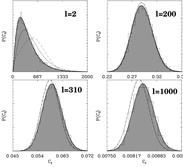
FIG. 3.: The pseudo–$C_{l}$ sampling pdfs , Eq. 21 (shaded), the $\chi^{2}$ (solid lines) and the Gaussian (dashed) approximations compared to Monte Carlo simulations (histograms) for l=2,200,310,1000. The theoretical $C_{l}$ were computed for the standard cold dark matter model($\Omega_{m}=1$, $\Omega_{b}h^{2}=0.015$, $H_{0}=70$km/s/Mpc). Note that the Monte Carlo simulations were run with noise pattern which strongly broke the azimuthal symmetry assumption. We nevertheless find superb agreement with our analytical predictions. The $\tilde{C}_{l}$ are in units of $\mu K$.

This becomes a more quantitative observation when looking at the percentage discrepancies between the mean and variances as a function of $l$ in Figure 4. The discrepancy is of the order of 1 % in the mean and 5% in the standard deviation on most scales, except for $l<70$ where the effect is larger. These discrepancies are important at the level of precision of future almost full sky missions. For medium and small sky coverage the mode couplings are stronger and we expect this to have an even larger effect on the probability distributions. We also compare the skewness $\beta_{1}$ and kurtosis $\beta_{2}$ of the $\chi^{2}$ distributions to our distributions. The percentage difference is larger than for the first two moments but arguably less important at large $l$, since $\beta_{1}$ and $\beta_{2}$ decay as $(2l+1)^{-\frac{1}{2}}$ and $(2l+1)^{-1}$, respectively.

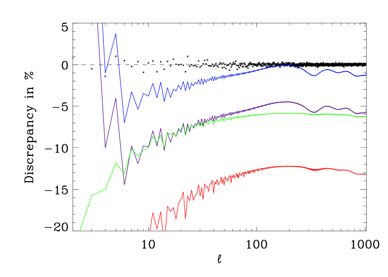
FIG. 4.: Percentage discrepancy of the first four moments of the pseudo–$C_{l}$ compared to the $\chi^{2}$ approximation as a function of angular wave number $l$. The solid lines are, top to bottom, the percentage discrepancy between the mean, standard deviation, skewness, and kurtosis of the $\chi^{2}$ approximation and the pseudo–$C_{l}$ distributions. The dashed line corresponds to 0% discrepancy. The stars are the $\langle\tilde{C}_{l}\rangle$ computed from 3328 Monte Carlo runs, showing excellent agreement only limited by Monte Carlo noise to better than 0.1 % for all $l$.

V Applications

A One–dimensional parameter estimation

As a first application we study the effect of approximating the likelihood for parameter estimation. Since our distributions have the correct means, we simply multiply them together for a simple, unbiased approximation to the likelihood

$$\tilde{{\cal L}}=\prod_{l}p(\tilde{C_{l}})$$ (25)

This is a conservative approximation in the sense that we will not overestimate the estimation accuracy since the marginal distributions have all correlations integrated out and we will therefore overestimate the error bars on the $C_{l}$. Using this likelihood, as well as the Gaussian and $\chi^{2}$ approximations, we attempt to estimate the baryon parameter $\Omega_{b}$ (holding all other parameters constant) from several randomly selected realizations in our MC pool. The results are shown in Figure 5. As expected, Gauss and $\chi^{2}$ consistently find estimates which are biased about 1.6% high, 3 standard errors of the mean away from the true value, while our likelihood gives a perfect fit.

Since the moment discrepancies depend on the underlying cosmological theory, this level of bias will also depend on the true theory. Therefore, this number should only be taken as indicative of the general level of the error introduced by using the naive Gaussian or $\chi^{2}$ approximations.

FIG. 5.: One parameter likelihood estimates of $\Omega_{b}$. Shown are the means (solid) within $\pm 3$ standard errors in the mean (dashed) of estimations from 17 realizations (diamonds) of the sky. Both the $\chi^{2}$ (left) and the Gaussian (right) approximations produce a bias, while our approximation (center) has no detectable bias.

B Multi–parameter estimation

We demonstrated in the previous subsection that we can use our formalism to construct approximate forms for the likelihood which lead to an unbiased parameter estimate. The idea proposed in this subsection is motivated by the fact that higher moments of the $\tilde{C}_{l}$ distributions die away quickly with $l$ (cf.  Eq. (19)) especially for observation geometries with large sky coverage. In particular we found in the case we studied that the distributions were visually indistinguishable from Gaussians for $l\gtrsim 100$. For parameters which are sensitive to high $l$ modes, we therefore further approximate Eq. (25) by replacing the pseudo–$C_{l}$ pdfs with Gaussians with the same mean and the same variance,

$$\widehat{\cal L}(C_{l})=\prod_{l>100}\exp\left[-\frac{\left(C_{l}-\left\langle{\tilde{C_{l}}}\right\rangle\right)^{2}}{\left\langle{\Delta\tilde{C}_{l}^{2}}\right\rangle}\right]$$ (26)

In this approximation, maximum likelihood estimation has reduced to simple $\chi^{2}$ fitting, however with the correct means and variances which implicitly account for inter-$C_{l}$ correlations.

The operation count for each likelihood evaluation has now dropped to $N_{pix}^{\frac{3}{2}}$. If the computation of the first and second pseudo-$C_{l}$ moments is organised in a memory–efficient manner the elements of the coupling matrix need to be computed only once. We find that we can evaluate Eq. (26) at a rate of several hundred times per hour. This surprisingly slow scaling of the computational cost with number of theories is presumably due to more efficient use of on–processor caching.

To illustrate, we solve the problem of estimating 3 parameters ($\Omega_{c}$ $\Omega_{b}$ and $H_{0}$) simultaneously from a sky with $12\times 10^{6}$ pixels. To compare with the naive Gaussian approach and to show that our method is unbiased, we compute maximum (approximate) likelihood estimates from 100 realisations of the sky and plot a representation of the the empirical distribution of parameter estimates in three dimensions in Figures 6 (naive $\chi^{2}$) and 7 (our approach).

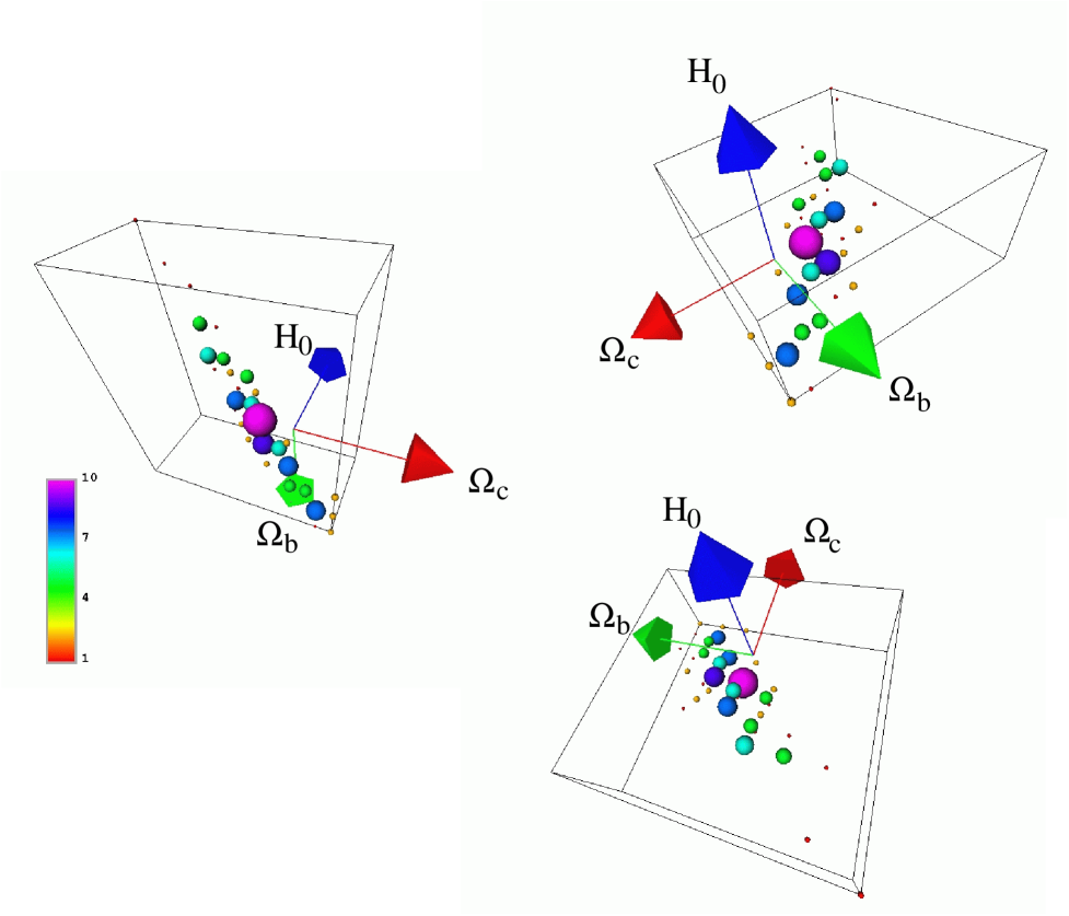
FIG. 6.: Multi–parameter estimation of $\Omega_{0}$, $\Omega_{b}$ and $H_{0}$ using naive $\chi^{2}$ fitting. The three panels show three views from different directions of the empirical distribution of the parameter estimates. Each sphere represents one bin of the three–dimensional distribution. The size and colour of a sphere indicates the number of realisations (out of 100 total) which led to parameter estimates within its bin. The true parameter values are at the origin of the coordinate axes. It is clearly visible that the distribution is shifted with respect to the true distribution by an amount which is inconsistent with the width of the distribution. In other words the true values could be ruled out at high significance if this estimate was used.

We find again that our approach is unbiased. The distributions of the estimates are clearly centered on the true values.

We stress that our approach avoids the usual difficulties of the Gaussian approximation as discussed in section III A. For example, even though we use the Gaussian approximation, which of course does not exclude negative $C_{l}$, they are assigned an exceedingly small probability. This is because no attempt is made to subtract out the noise contribution from the pseudo–$C_{l}$ — instead it is modeled consistently and the (signal$\times$noise) cross term which is present in each realisation is not allowed to dominate.

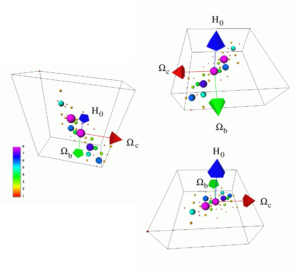
FIG. 7.: Multi–parameter estimation of $\Omega_{0}$, $\Omega_{b}$ and $H_{0}$ using our approximate likelihood Eq. (26). The three panels show three views from different directions of the empirical distribution of the parameter estimates. Each sphere represents one bin of the three–dimensional distribution. The size and colour of a sphere indicates the number of realisations (out of 100 total) which led to parameter estimates within its bin. The true parameter values are at the origin of the coordinate axes. It is clearly visible that the distribution is correctly centered on the true values.

C Test for non–Gaussianity

We now mention an application which reverses our way of thinking about the results in this paper and takes advantage of the exact analytical expressions we compute for the pseudo–$C_{l}$ distributions. Imagine that we have gained knowledge that a certain theory is correct, for example through measurements of the large scale structure of the galaxy distribution and other probes of cosmology such as supernovae etc. Then we can use the formalism shown here as a test of Gaussianity, simply by computing the pseudo–$C_{l}$ and then substituting them into Eq. (21). An interesting feature is that this probes Gaussianity scale by scale which might make it feasible to disentangle confusion effects if the non–Gaussian signal was only apparent on a small range of scales and masked by a Gaussian component on other scales.

D De–biasing

In the introduction we mentioned the use of iterative methods to attack the difficult problem of power spectrum estimation. A good starting guess can drastically speed up the convergence of such methods. In the case of large sky coverage, where the biases which occur in the $\tilde{C}_{l}$ are small, we suggest the following recipe as a “poor man’s power spectrum estimator” for de–biasing the power spectrum in only ${\cal O}\left(N_{pix}^{\frac{3}{2}}\right)$ computational time:

1. compute the $\tilde{C}_{l}$ from the data,

2. fit a smooth curve $C^{smooth}_{l}$ through them,

3. compute ${C}^{s}_{l}=(\tilde{C}_{l}-C^{noise}_{l})$ and set all negative ${C}^{s}_{l}$ to zero,

4. use the ${C}^{s}_{l}$ instead of $C^{theory}_{l}$ in Eq. (19) to compute $\langle\tilde{C}_{l}\rangle$.

Then

$$\hat{C}_{l}=\tilde{C}_{l}+(C^{smooth}_{l}-\langle\tilde{C}_{l}\rangle)$$ (27)

is an estimator of the underlying theory $C_{l}$. There is a tiny residual bias which is second order in the discrepancy shown in Figure 4. This is utterly negligible for upcoming satellite missions.

VI Further discussion and conclusions

We have computed the sampling properties of a set of quantities which we call pseudo–$C_{l}$. We have shown the usefulness of these quantities for the easy compression of large Cosmic Microwave Background data sets as well as for the forecasting of the discriminatory power of planned experiments. For example, in situation where percentage accuracy is required, the pseudo–$C_{l}$ sample variances shown in Figure 4 could immediately replace the usual approximation which simply rescales the cosmic variances for the full sky by the sky fraction.

On the other hand this exact framework can be used to justify or derive more approximate methods. We have given an example for the construction of an approximate but unbiased likelihood for cosmological parameters on the basis of a Gaussian approximation to the marginalised pseudo–$C_{l}$ probability distributions. Using this approximation we can evaluate the likelihood for hundreds of theories per hour on a single CPU and find unbiased estimates.

If only a rough treatment of the $C_{l}$ statistics is sufficient, for example in the case of large sky coverage, the results derived here can be used as a justification for other simplifying assumptions which are already in use in the literature.

Apart from the obvious applications to experiments with small and medium sky coverage such as balloons or ground–based missions, many further uses of this framework are conceivable. For example, one could use the statistical framework to design ’optimal’ scanning strategies, encoded in $W_{N}$, and assess more realistically if secondary anisotropies will be detectable with future CMB missions. Finally, all ingredients are there to refine the approximation to the joint likelihood we used in this paper by taking into account the covariances Eq. (24), for example by using a multivariate Edgeworth expansion around the peak of the likelihood.

We note that numerical techniques have recently been developed [23] which allow the computational solution of the power spectrum estimation for high $l$ applications under similar assumptions to the ones which lead to the analytical results derived in this paper. Their methods are efficient for the case of almost full sky observations. A purely numerical approach still requires significant computational resources, especially if there is signal in modes with $l>1000$. The results presented in this paper should be seen as complementary to such calculations. An analytical framework admits a more fundamental approach to understanding and is a useful yardstick against which numerical work can be tested or from which approximate methods can be derived as we have demonstrated in the applications presented in section V.

Our methods do not allow for significantly correlated noise. Due to the current state of detector technology, all CMB missions suffer from correlated noise, with the possible exception of the MAP satellite [24]. Apart from brute force numerical calculation with ${\cal O}\left(N_{pix}^{3}\right)$ operations, which is no longer feasible even with current experiments, there are currently no techniques for computing sampling statistics in the presence of correlated noise. This clearly needs to be addressed as an extremely urgent and important issue.

To summarize, we have presented a theoretical framework for the study of power spectrum statistics which is applicable regardless of the size of the sky area covered. We go beyond current approximations and present a semi–analytic formalism for the computation of sampling distributions of the $C_{l}$ for any Gaussian cosmological model and a large and important class of surveying strategies. We show that these results can be usefully applied to the estimation of cosmological parameters from simulated data. A range of further applications is suggested which demonstrate the power of our formalism.

A Low order non–cosmological modes

We assume in this paper that we have access to a partial sky map of CMB anisotropies free from non–cosmological signal. Even in the event that foreground contributions can be filtered out using the frequency information provided by multi–channel experiments, this assumption merits further discussion — particularly for large amplitude low order modes such as the monopole and the dipole which are thought to consist exclusively of non-cosmological signal.

An ideal full sky map of the cosmic microwave background anisotropies has zero mean, by definition. Also, in Friedmann–Robertson–Walker models, there is no cosmological dipole. But we expect realistic maps resulting from observations of the microwave sky to contain both monopole and dipole components; Galactic emission is positive definite and will therefore give a monopole contribution. The motion of our solar system with respect to the frame in which the CMB is at rest produces a dipole. The question arises how to deal with the presence of such non–cosmological low order modes.

If the experiment measures total power, we may hope to remove a sizeable part of the monopole using the frequency information of a multi–channel experiment. In the case of a differential experiment such as MAP which is blind to the monopole component, the problem depends on the particulars of the map–making algorithm employed. Frequency information alone cannot distinguish between a non-cosmological and a spurious dipole since both are due to the microwave background. Studies of the peculiar velocity field may provide some information.

We see the three following different approaches which can be used to deal with the problem of mode to mode coupling when non–cosmological components are removed from the sky.

One is orthogonalisation [13]. This solves the problem, but is not feasible computationally when dealing with millions of degrees of freedom.

The other is projecting out the undesired modes either by fitting and subtracting or more formally by operating with projection operators. Those approaches lead to a correlation structure for the remaining modes which is not analytically tractable in the manner presented in this paper.

The third is allowing for the presence of a monopole and a dipole in a Bayesian fashion, by including a rough estimate of their size in the theory $C_{l}$. In particular, a rough a priori measure of the monopole and dipole present in the data can be input into $C_{0}$ and $C_{1}$. Our statistical framework allows this and yields the correct predicted sampling statistics for all $C_{l}$ taking into account all the $l$–$l^{\prime}$ couplings due to the cut. In effect, $C_{0}$ and $C_{1}$ are treated as nuisance parameters which are marginalised over in our formalism.

This will change the sampling statistics of low order modes predicted by our theory in a self-consistent way. Cosmological parameters can then be estimated in an unbiased fashion without monopole or dipole removal. Whether this is feasible in practice would be an interesting avenue for further study. We are not aware of any existing fast method which offers a similarly consistent treatment.

In practice we observe that for large sky coverage the entries of the coupling matrices diminish rapidly with increasing $l$. To a good approximation, modes with $l\gtrsim 100$ are therefore unaffected by the presence or absence of low order modes, $l<2$. One of the main applications of our formalism has been to the estimation of parameters which depend mostly on the shape of the $C_{l}$ spectrum around and beyond the first acoustic peak. These analyses are unaffected by the details of how low order modes of non–cosmological origin are dealt with.

B Factorising the correlation matrix

For a general azimuthally symmetric window $W(\theta)$ we can write the $\tilde{C}_{l}$ as

$$\begin{split}\tilde{C}_{l}=\sum_{m}\int d\Omega_{1}W(\theta_{1})\int&d\Omega_{2}W(\theta_{2})Y_{lm}({\bf{\gamma}}_{1})Y^{\ast}_{lm}({\bf{\gamma}}_{2})\\ &\sum_{l^{\prime}m^{\prime}}\sum_{l^{\prime\prime}m^{\prime\prime}}a_{l^{\prime}m^{\prime}}a^{\ast}_{l^{\prime\prime}m^{\prime\prime}}Y_{lm}({\bf{\gamma}}_{1})Y^{\ast}_{l^{\prime\prime}m^{\prime\prime}}({\bf{\gamma}}_{2})\end{split}$$ (B1)

We define normalised associated Legendre polynomials $\lambda_{lm}(x)$ in Appendix C and use the notation $\mu=\cos\theta$. Then $Y_{lm}(\theta,\phi)=\lambda_{lm}(\mu)e^{im\phi}$ and we notice that the Kronecker–$\delta$ from the azimuthal integration select only one term out of the sums over $m^{\prime}$ and $m^{\prime\prime}$, namely

$$\tilde{C}_{l}=\sum_{m}\left(\sum_{l^{\prime}=0}^{\infty}a^{\ast}_{l^{\prime}m}{\cal W}_{l^{\prime}m}^{(l)}\right)\left(\sum_{l^{\prime\prime}=0}^{\infty}a_{l^{\prime\prime}m}{\cal W}_{l^{\prime\prime}m}^{(l)}\right)$$ (B2)

where the

$${\cal W}_{l^{\prime}m}^{(l)}\equiv W_{l^{\prime}m\;lm}=\int d\mu W(\mu)\lambda_{lm}(\mu)\lambda_{l^{\prime}m}(\mu)$$ (B3)

are real matrices. Because the $W$ matrices are real, the terms in the brackets are complex conjugates of each other and we obtain Eq. (10) as desired.

C Algorithm for computing the coupling matrix

Subsection C 1 reviews some useful properties of spherical harmonics. In subsection C 2 we derive an efficient algorithm for computing the coupling matrix Eq. (B3) due to an azimuthally symmetric mask, Eq. (C16). More general windows can be piecewise defined in terms of masks of varying height. The corresponding coupling matrices are then suitably weighted sums over the coupling matrices due to the individual masks.

1 Some properties of spherical harmonics

The Spherical Harmonics are

$$Y_{lm}(\theta,\phi)=\lambda_{lm}(\cos\theta){\rm{e}}^{{i}m\phi}$$ (C1)

where the

$$\lambda_{lm}(x) = \sqrt{\frac{2l+1}{4\pi}\frac{(l-m)!}{(l+m)!}}P_{lm}(x),\quad{\rm for}\,m\geq 0$$ (C2)

$$\lambda_{lm} = (-1)^{m}\lambda_{l|m|},\quad{\rm for}\,m\geq 0,$$ (C3)

$$\lambda_{lm}=0,\quad{\rm for}\,|m|>l.$$ (C4)

In the following we will only consider positive $m$. The associated Legendre Polynomials $P_{lm}$ are defined as

$$P_{lm}(x)=(-1)^{m}(1-x^{2})^{m/2}\frac{d^{m}}{dx^{m}}P_{l\ }(x),$$ (C5)

where $P_{l\ }$ is the Legendre function of the first kind defined as

$$P_{l\ }(x)=\frac{1}{2^{l}l!}\frac{d^{l}}{dx^{l}}(x^{2}-1)^{l}.$$ (C6)

They are solution of the differential equation

$$(1-x^{2})\frac{d^{2}}{dx^{2}}P_{lm}-2x\frac{d}{dx}P_{lm}+\left(l(l+1)-\frac{m^{2}}{1-x^{2}}\right)P_{lm}=0$$ (C7)

Definition Eq. (C5) leads to a large number of relations between polynomials of different order $l$ and $m$ and their derivatives. Among them the following two will be useful (see, e.g.  [22] §8.700)

$$P_{lm}=-\frac{x(m-1)}{\sqrt{1-x^{2}}}P_{l(m-1)}-\sqrt{1-x^{2}}\frac{d}{dx}P_{l(m-1)}$$ (C8)

and

$$(1-x^{2})\frac{d}{dx}P_{lm}=-lxP_{lm}+(l+m)P_{(l-1)m}$$ (C9)

It is possible to obtain the $P_{lm}$ or alternatively the $\lambda_{lm}$ through relations that raise from the fact that they are orthogonal polynomials. The following recurrence is stable and very convenient for numerical uses :

starting with $\lambda_{00}=1/\sqrt{4\pi}$

$$\lambda_{mm} = -\sqrt{\frac{2m+1}{2m}}\,\sqrt{1-x^{2}}\,\lambda_{(m-1)(m-1)}$$ (C10)

$$\lambda_{(m+1)m} = x\,\sqrt{2m+3}\,\lambda_{mm}$$ (C11)

$$\lambda_{lm} = \left[x\lambda_{(l-1)m}-\frac{\lambda_{(l-2)m}}{A(l-1,m)}\right]A(l,m)\quad{\rm with}\quad A(l,m)=\sqrt{\frac{4l^{2}-1}{l^{2}-m^{2}}}$$ (C12)

2 Scalar product on the cut sphere

The spherical harmonics have the property that they are an orthonormal basis spanning the Hilbert space of square integrable functions on the sphere $S^{2}$, i.e.  their scalar product is the identity matrix:

$$\int_{0}^{2\pi}d\phi\int_{-1}^{1}d\cos\theta Y_{l^{\prime}m^{\prime}}(\theta,\phi)Y_{lm}(\theta,\phi)=\delta_{l^{\prime}l}\delta_{m^{\prime}m}$$ (C13)

Let us now define the cut sphere scalar product of spherical harmonics under a mask or window $W$

$$A_{l^{\prime}l}^{mm^{\prime}}[W]\equiv\int_{0}^{2\pi}d\phi\int_{-1}^{1}d\cos\theta\,W(\theta,\phi)Y_{l^{\prime}m^{\prime}}(\theta,\phi)Y_{lm}(\theta,\phi)$$ (C14)

In the following we will consider only a sharp ’strip’ filter whose boundaries are parallel to the equator (but not necessarily symmetric about the equator).

$$W(\cos\theta)=W(x) = 1\quad{\rm if}\,a\leq x\leq b$$ (C15)

$$= 0\quad{\rm otherwise}$$ (C16)

This is simply related to physically relevant windows. For example a straight cut removing foregrounds concentrated around the Galactic disk is modeled by $\tilde{W}=1-W$ with $a=-b$ setting the width of the cut. Because $A_{l^{\prime}l}^{mm^{\prime}}[\tilde{W}]={\bf 1}-A_{l^{\prime}l}^{mm^{\prime}}[W]$, where ${\bf 1}=\delta_{l^{\prime}l}\delta_{m^{\prime}m}$, everything that follows can be translated to this window with the replacements

$$b\leq a,\quad{\rm and}\,A_{-1\ }^{-1}[\tilde{W}]=1.$$ (C17)

Because the window Eq. (C16) is independent of $\phi$ it preserves the azimuthal symmetry and only spherical harmonics with the same $m$ are coupled. The non–trivial terms of the coupling matrix $A$ are then

$$A_{l^{\prime}l}^{m} = 2\pi\int_{a}^{b}dx\,\lambda_{l^{\prime}m}(x)\lambda_{lm}(x)$$ (C18)

$$= \frac{\sqrt{(2l^{\prime}+1)(2l+1)}}{2}\sqrt{\frac{(l^{\prime}-m)!(l-m)!}{(l^{\prime}+m)!(l+m)!}}\,I_{l^{\prime}l}^{m}(a,b)$$ (C19)

where

$$I_{l^{\prime}l}^{m}(a,b)\equiv\int_{a}^{b}dx\,P_{l^{\prime}m}(x)P_{lm}(x)$$ (C20)

This expression is symmetric under interchange of $l^{\prime}$ and $l$ and under $m\rightarrow-m$. If $0\leq l\leq l_{max}$ this implies that, asymptotically for large $l_{max}$ there are $\frac{l_{max}^{3}}{6}$ independent components of $I_{l^{\prime}l}^{m}(a,b)$. If the window $W$ is symmetric around the equator and therefore preserves reflection symmetry, only multipoles with the same parity of $l$ couple to one another, and the number of non–trivial elements reduces to $\sim l_{\rm max}^{3}/12$.

The problem of evaluating all independent components of Eq. (C20) is to find a way of computing the integrals Eq. (C20) without having to take recourse to time–consuming numerical quadratures.

If one substitutes Eq. (C8) for $P_{lm}$ and $P_{l^{\prime}m}$ in Eq. (C20), integrates by parts to exhibit the second derivative of $P_{l(m-1)}$, and makes use of the differential equation Eq. (C7) one obtains

$$I_{l^{\prime}l}^{m}(a,b) = -(m+l)(m-l-1)I_{l^{\prime}l}^{m-1}(a,b)$$ (C21)

$$+ (m-l-1)\left[{xP_{l^{\prime}(m-1)}P_{l(m-1)}}\right]_{a}^{b}$$ (C22)

$$+ (m+l-1)\left[{P_{l^{\prime}(m-1)}P_{(l-1)(m-1)}}\right]_{a}^{b}$$ (C23)

where we used Eq. (C9) to simplify the last two terms.

This can be simplified further in the case $l\not=l^{\prime}$, by noting that the left hand side of Eq. (C23) is by definition symmetric in $l^{\prime},l$ whereas the right hand side is not explicitly symmetric. So, by subtracting Eq. (C23) from itself after swapping $l$ and $l^{\prime}$ one obtains

$$I_{l^{\prime}l}^{m}(a,b) = \left((l^{\prime}-l)\left[{xP_{l^{\prime}m}P_{lm}}\right]_{a}^{b}+(l+m)\left[{P_{l^{\prime}m}P_{(l-1)m}}\right]_{a}^{b}-(l^{\prime}+m)\left[{P_{(l^{\prime}-1)m}P_{lm}}\right]_{a}^{b}\right)$$ (C24)

$$/ \left({l^{\prime}}^{2}+l^{\prime}-l^{2}-l\right)\quad{\rm for}\,\,l^{\prime}\not=l.$$ (C25)

The diagonal terms ($I_{l\ }^{m}(a,b)=\int_{a}^{b}P_{lm}P_{lm}$) can be obtained thanks to the recurrence relation

$$(l-m)P_{lm}=x(2l-1)P_{(l-1)m}-(l+m-1)P_{(l-2)m}.$$ (C26)

One obtains a recurrence on the diagonal terms involving also the off–diagonal terms computed by Eq. (C25).

$$I_{l\ }^{m}(a,b) = \left(\frac{2l-1}{2l+1}\right)\left(\frac{l+m}{l-m}\right)I_{l-1\ }^{m}(a,b)$$ (C27)

$$+ \left(\frac{2l-1}{2l+1}\right)\left(\frac{l-m+1}{l-m}\right)I_{(l+1)(l-1)}^{m}(a,b)-\frac{l+m-1}{l-m}I_{l(l-2)}^{m}(a,b)$$ (C28)

To conclude, the elements of the coupling matrix $A$ are given in terms of recurrence relations as follows. For $m\not=m^{\prime}$ we have

$$A_{l^{\prime}l}^{m^{\prime}m}=0,$$

while for $l\not=l^{\prime}$

$$\begin{split}A_{l^{\prime}l}^{m}&=\Biggl{(}(l^{\prime}-l)\left[{x\lambda_{l^{\prime}m}\lambda_{lm}}\right]_{a}^{b}+\sqrt{\frac{2l+1}{2l-1}(l^{2}-m^{2})}\left[{\lambda_{l^{\prime}m}\lambda_{(l-1)m}}\right]_{a}^{b}-\\ &\quad\quad\quad\quad\quad\sqrt{\frac{2l^{\prime}+1}{2l^{\prime}-1}({l^{\prime}}^{2}-m^{2})}\left[{\lambda_{(l^{\prime}-1)m}\lambda_{lm}}\right]_{a}^{b}\Biggr{)}\times\frac{2\pi}{(l^{\prime}-l)(l^{\prime}+l+1)},\end{split}$$ (C29)

and all other cases are given by

$$\begin{split}A_{l\ }^{m}&=A_{l-1\ }^{m}+\sqrt{\frac{2l-1}{2l+3}\frac{(l+1)^{2}-m^{2}}{l^{2}-m^{2}}}A_{(l+1)(l-1)}^{m}-\sqrt{\frac{2l+1}{2l-3}\frac{(l-1)^{2}-m^{2}}{l^{2}-m^{2}}}A_{l(l-2)}^{m}\quad(l>m)\\ A_{m\ }^{m}&=A_{m-1\ }^{m-1}+\frac{2\pi}{2m+1}\left[{x\lambda_{mm}\lambda_{mm}}\right]_{a}^{b}\end{split}$$ (C30)

with $A_{-1\ }^{-1}[W]\equiv 0$. As only a few operations are needed to evaluate each of these terms, calculating the whole coupling matrix costs $O(l_{\rm max}^{3})$ operations and only requires about 10 minutes for $l_{\rm max}=2048$ on a fast work–station.

D The method of characteristic functions

1 Densities of functions of random variates

How do we approach computing the probability density function (pdf) of a (set of) continuous random variate(s) which can itself be written as a function of one or more random variates whose pdfs are known? The usual expression for changing the measure is

$$p(f(x))=p(x)\left|\frac{\partial f}{\partial x}\right|^{-1}$$ (D1)

where $\left|\frac{\partial f}{\partial x}\right|$ is the Jacobian of the transformation. However this expression is inconvenient if the transform is not monotonic or the number of transformed variates is not the same as the number of original variates.

In order to attack this more general situation we replace Eq. (D1) by a more powerful integral expression. The idea here is to define an ”atomic” pdf which allows for only one event. For a continuous variate this is the delta function. The sum of these ”atoms” over all possible outcomes, weighted with the probability that the underlying variates produce this outcome gives the resulting pdf. In symbols, if the $n$ underlying variates $X=\{x_{i},i=1,\dots,n\}$ have the joint pdf $p(X)$, then the pdf of $z=f(X)$ is

$$p(z)=\int\delta\left(z-f(X)\right)p(X)dX,$$ (D2)

where $dX$ denotes $\prod_{i=1}^{i=n}dx_{i}$.

2 The Method of characteristic functions

In particular we are often interested in the distribution of a linear combination of $n$ independent quantities whose distributions are known. Computing these distributions is now straightforward – we can apply Eq. (D2) with the simplification that $f(X)$ is linear and p(X) factorises owing to the independence of the variates. The trick is to perform the resulting convolution in Fourier space by application of the Fourier convolution theorem. This is far easier to do than computing $n$ convolutions, at least if $n>2$. The Fourier transform of a pdf of a variate is called its characteristic function — hence the name of the method. All major pdfs have tabulated Fourier transforms. This makes this method very simple to apply, up to the final step of inverse transforming to obtain the required pdf. This may be tabulated too. If not, extending the integrand to the complex plane and using contour integration perhaps after expanding into partial fractions may lead to success. In any case, at least only one integral needs to be evaluated compared to $n$ for the direct convolution.

Even if the inverse transform does not succeed, all is not lost. A key fact about characteristic functions allows us to gain as much information as we like about the statistical properties of $z$. By formally computing the Maclaurin series of the Fourier transform which defines the characteristic function $c(k_{z})$ of a variate $z$, we find that it is the generating function for its statistical moments,

$$c(k_{z})=\sum_{n=0}^{n=\infty}\left\langle{z^{n}}\right\rangle\frac{(ik_{z})^{n}}{n!}.$$ (D3)

Therefore, the moments can be obtained by straightforward differentiation of $c(k_{z})$. Equivalently, and sometimes more conveniently, the natural logarithm of the characteristic function generates the cumulants of the distribution. Moments and cumulants are algebraically simply related. Once these moments or cumulants are known there is a host of methods for using them to approximate $p(z)$ [21]. In particular, when $n$ is large, the large number theorem states that $p(z)$ approaches a Gaussian with mean $\left\langle{z}\right\rangle$ and variance $\left\langle{z^{2}}\right\rangle$ (under weak conditions on the $p_{i}(x_{i})$).

REFERENCES

-
[1]
For a compendium of links to experiments refer to e.g.
http://www.mpa-garching.mpg.de/banday/CMB.html
or
http://www.sns.ias.edu/max/cmb/experiments.html. - [2] C. L. Bennett et al., “Microwave Anisotropy Probe: A MIDEX Mission Proposal”, 1996, see also http://map.gsfc.nasa.gov/.
- [3] Bersanelli et al., “COBRAS/SAMBA: Report on the Phase A Study”, 1996, see also http://astro.estex.esa.nl/Planck/.
- [4] L. E. Knox, Phys. Rev. D52, 4307 (1995).
- [5] G. Jungman et al., Phys. Rev. D54, 1332 (1995).
- [6] M. Zaldarriaga, D. Spergel, and U. Seljak, Astrophys. J. 488, 1 (1997).
- [7] J. R. Bond, G. Efstathiou, and M. Tegmark, MNRAS 291, L33 (1998).
- [8] C. H. Lineweaver and D. Barbosa, A&A 329, 799 (1998).
- [9] C. H. Lineweaver and D. Barbosa, ApJ496, 624 (1998).
- [10] R. Stompor and G. Efstathiou, MNRAS 302, 735 (1999).
- [11] A. J. Banday et al., Astrophys. J. 475, 393 (1997).
- [12] K. M. Górski, Astrophys. J. Lett. 430, L85 (1994).
- [13] K. M. Górski et al., Astrophys. J. Lett. 430, L89 (1994).
- [14] K. M. Górski, (1997), proceedings of the XXXIst Recontres de Moriond, ”Microwave Background Anisotropies”.
- [15] J. R. Bond, A. H. Jaffe, and L. E. Knox, Phys. Rev. D57, 2117 (1998).
- [16] J. Borrill, Phys. Rev. D59, 027302 (1999).
- [17] M. Tegmark, Phys. Rev. D55, 5895 (1997).
- [18] J. R. Bond, A. H. Jaffe, and L. E. Knox, 1998, astro-ph/9808264.
- [19] P. J. E. Peebles, Astrophys. J. 185, 413 (1973).
- [20] M. G. Hauser and P. J. E. Peebles, Astrophys. J. 185, 757 (1973).
- [21] A. Stuart and J. K. Ord, Advanced Theory of Statistics (Edward Arnold, London, 1994).
- [22] I. S. Gradshteyn and I. M. Ryzhik, Table of Integrals, Series and Products (Fifth Edition) (Academic Press, London, 1994).
- [23] S. P. Oh, D. N. Spergel, and G. Hinshaw, ApJ510, 551 (1999).
- [24] L. Page, 1998 (private communication).