Structure of Dark Matter Halos From Hierarchical Clustering

Abstract

We investigate the structure of the dark matter halo formed in the cold dark matter scenario using $N$-body simulations. We simulated 12 halos with the mass of $6.6\times 10^{11}M_{\odot}$ to $8.0\times 10^{14}M_{\odot}$. In almost all runs, the halos have density cusps proportional to $r^{-1.5}$ developed at the center, which is consistent with the results of recent high-resolution calculations. The density structure evolves in a self-similar way, and is universal in the sense that it is independent of the halo mass and initial random realization of density fluctuation. The density profile is in good agreement with the profile proposed by Moore et al. (1999), which has central slope proportional to $r^{-1.5}$ and outer slope proportional to $r^{-3}$. The halo grows through repeated accretion of diffuse smaller halos. We argue that the cusp is understood as a convergence slope for the accretion of tidally disrupted matter.

1 Introduction

In standard cosmological pictures, such as the cold dark matter cosmology, dark matter halos are considered to be formed in a hierarchical way; smaller halos first formed from initial density fluctuations and they merged with each other to become larger halos. In reality, the formation process of dark matter halo is rather complicated, since a variety of processes, such as merging between halos of various sizes and tidal disruption of small halos (satellite) proceed simultaneously.

One of the most influential works on the dark matter halo is the ”finding” of the universal profile by Navarro, Frenk, and White (1996, 1997, hereafter NFW), though there were many analytical and numerical studies before NFW (see NFW (1996) or Bertschinger (1998) for reviews). NFW performed $N$-body simulations of the halo formation and found that the profile of dark matter halo can be fitted by a simple formula

$$\rho={\rho_{0}\over(r/r_{\rm s})(1+r/r_{\rm s})^{2}},$$ (1)

where $\rho_{0}$ is a characteristic density and $r_{\rm s}$ is a scale radius. They also argued that the profile has the same shape, independent of the halo mass, the initial density fluctuation spectrum or the value of the cosmological parameters. It should be noted that, before NFW, Dubinski and Carlberg (1991) also found in their high-resolution simulation the halo can be well fitted by Hernquist (1990) profile .

Many studies on the NFW ”universal profile”, both numerical and analytical, were done after their proposal. Many $N$-body simulations whose resolution are similar to those of NFW were performed and results similar to NFW were obtained (Cole and Lacy 1996, Tormen, Bouchet and White 1996, Brainerd, Goldberg, and Villumsen 1998, Thomas et al. 1998, Okamoto and Habe 1999, Huss, Jain and Steinmetz 1999, Kravtov et al. 1998, Jing 2000). Analytical and semi-analytical studies to explain the NFW universal profile were also done (Evans and Collet 1997, Syer and White 1998, Avila-Reese, Firmani, Hernandez 1998, Nusser and Sheth 1999, Kull 1999, Heriksen and Widrow 1999, Yano and Gouda 1999, Bullock et al. 1999, Subramanian, Cen, Ostriker 2000, Lokas 2000). The clear understanding for the NFW profile, however, has not yet been given. One of the reasons why a clear understanding has not been established might be that all these studies were trying to answer a wrong question.

Our previous study (Fukushige and Makino 1997, hereafter FM97) showed that density profile obtained by high-resolution $N$-body simulation is different from the NFW universal profile. We performed simulations with 768k particles, while previous studies employed $\sim 20$k. We found that the galaxy-sized halo has a cusp steeper than $\rho\propto r^{-1}$.

This disagreement with the NFW universal profile was confirmed by other high-resolution simulations. Moore et al. (1998, 1999) and Ghigna et al. (2000) performed simulations with up to 4M particles and obtained the results similar to ours. They found that cluster-sized halos also have cusps steeper than the NFW profile and they proposed the modified universal profile, $\rho=\rho_{0}/[(r/r_{\rm s})^{1.5}(1+(r/r_{\rm s})^{1.5})]$. On the other hand, Jing and Suto (2000) found that the density profile of dark matter is not universal. They performed a series of $N$-body simulations and concluded that the power of the cusp depends on mass. It varies from $-1.5$ for galaxy mass halo to $-1.1$ for cluster mass halo.

In this paper, we again investigate the structure of dark matter halos using $N$-body simulation. We performed $N$-body simulations of formation of 12 dark matter halos with masses $6.6\times 10^{11}M_{\odot}$ to $8.0\times 10^{14}M_{\odot}$, using a special-purpose computer GRAPE-5 (Kawai et al. 2000) and Barnes-Hut treecode. In section 2, we describe the model of our $N$-body simulation. In section 3, we present the results of simulation. Section 4 is for summary and section 5 is for discussion.

2 Simulations Models

We performed in total 12 runs on 4 different mass scales, which are summarized in Table 1. Initial conditions were constructed in a way similar to that in FM97. We assigned initial positions and velocities to particles in a spherical region with a radius of $R$ Mpc surrounding a density peak selected from a unconstrained discrete realization of the standard CDM model ($H_{o}=50$km/s/Mpc, $\Omega=1$ and $\sigma_{8}=0.7$). The peak was chosen from an $R_{\rm box}$ Mpc cube using a density field smoothed by a Gaussian filter of radius ($R_{\rm box}/2$) Mpc. The values of $R$ and $R_{\rm box}$ in the comoving flame are summarized in Table 1. In order to generate the discrete realization of the CDM model we used the COSMICS package.

Table 1: Simulation Models

Run	$R$ (Mpc)	$R_{\rm box}$ (Mpc)	$m$ ($M_{\odot}$)	$\varepsilon$ (kpc)	$\Delta t$ (yr)	$z_{\rm start}$	$z_{\rm end}$
16M0	12.8	32	$3.0\times 10^{8}$	0.56	$1.6\times 10^{6}$	18.8	0.0
16M1	16	32	$6.0\times 10^{8}$	0.56	$1.5\times 10^{6}$	18.5	0.0
16M2	16	32	$6.1\times 10^{8}$	0.56	$1.6\times 10^{6}$	20.4	0.0
8M0	6.4	16	$3.7\times 10^{7}$	0.28	$7.9\times 10^{5}$	22.3	0.58
8M1	8	16	$7.6\times 10^{7}$	0.28	$7.5\times 10^{5}$	22.2	0.63
8M2	8	16	$7.6\times 10^{7}$	0.28	$7.8\times 10^{5}$	23.9	0.59
4M0	3.2	8	$4.7\times 10^{6}$	0.14	$7.8\times 10^{5}$	25.9	1.6
4M1	4	8	$9.5\times 10^{6}$	0.14	$7.4\times 10^{5}$	25.9	1.6
4M2	4	8	$9.5\times 10^{6}$	0.14	$7.6\times 10^{5}$	27.4	1.2
2M0	1.6	4	$5.9\times 10^{5}$	0.07	$3.8\times 10^{5}$	29.7	2.1
2M1	2	4	$1.2\times 10^{6}$	0.07	$3.6\times 10^{5}$	29.7	2.2
2M2	2	4	$1.2\times 10^{6}$	0.07	$3.8\times 10^{5}$	30.9	1.8

We followed evolution of the density peak by $N$-body simulation. We added the local Hubble flow and integrated the orbits directly in the physical space. We used the Plummer softened potential with the softening length constant in physical space, and used a leap-flog integrator with shared and constant timestep. In Table 1 we summarized the individual particle mass, $m$, softening length, $\varepsilon$, timestep size, $\Delta t$, and starting and ending redshift, $z_{\rm start}$ and $z_{\rm end}$. The masses of particles are equal and the total number of particles for each simulation is $(2.0-2.1)\times 10^{6}$.

We determined the radius $R$ Mpc for Run 16M{0,1,2} using trial runs with smaller number of particles, so that all particles lying inside of $r_{200}$ at $z_{\rm end}$ are included. Here, the radius $r_{200}$ is defined as the radius of the sphere in which the mean density $\rho$ is equal to $200\rho_{\rm crit}$, where $\rho_{\rm crit}$ is the critical density. We did not include tidal effects from outside the $R$ Mpc sphere. The region of Runs 8M{0,1,2}, 4M{0,1,2}, and 2M{0,1,2} is 1/2, 1/4, and 1/8 of the size of 16M{0,1,2} and mass resolution are $\times 2$, $\times 4$, and $\times 8$, respectively. The ending redshift $z_{\rm end}$ for Runs 8M{0,1,2}, 4M{0,1,2}, and 2M{0,1,2} is determined so that the truncation outside the sphere did not influence the profile around $r_{200}$.

The number before M in a run name (ex. 8 for Run 8M1) indicates the length of the simulation box, $R_{\rm box}/2$, in Mpc. The number after M in the run name (ex. 1 for Run 8M1) identifies the index for the random number seed used to generate initial density field. For example, Runs {16,8,4,2}M0 are series of runs in which the phases of initial density waves are same and the amplitude of the wave are different.

For the force calculation, we used the Barnes-Hut tree code ($\theta=0.75$, Barnes and Hut 1986, Barnes 1990, Makino 1991) implemented on GRAPE-5 (Kawai et al. 2000), a special-purpose computer designed to accelerate $N$-body simulations. Using the tree code on two GRAPE-5 boards and a workstation whose CPU is 21264/677MHz Alpha chip, one timestep took 21 seconds. The total number of timesteps is about $6000-8000$. Therefore, we can complete one run in 35-50 CPU hours.

3 Result

3.1 Snapshot

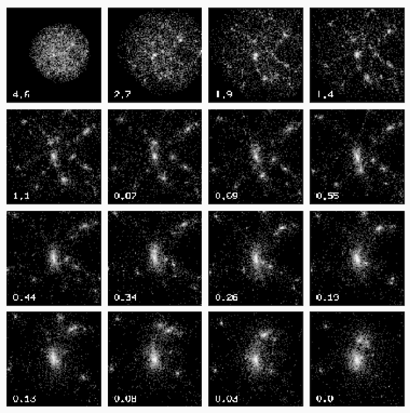
Figure 1: Snapshots from Run 16M0 at 16 different redshifts indicated by the number at lower-left of each panel. The length of the side for each panel is equal to $4r_{200}$ at $z_{\rm end}$.

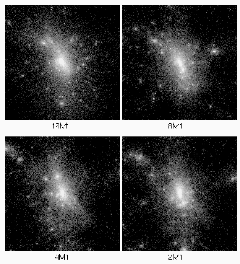
Figure 2: Snapshots from Runs {16,8,4,2}M1 at the final redshifts. The length of the side for each panel is equal to $4r_{200}$ at $z_{\rm end}$.

Figure 1 shows the particle distributions for Run 16M0 at 16 different redshifts. For these plots, we shifted the origin of coordinates to the position of the potential minimum so that the largest halo is at the center of the panel. Figure 2 shows the particle distribution for Runs {16,8,4,2}M1 together. The phases of waves for initial density field are the same for all these runs and only the amplitude are different. In Table 2, we summarized the radius $r_{200}$, the mass $M_{200}$ and number of particles $N_{200}$ within $r_{200}$, at $z_{\rm end}$.

Table 2: Halo properties at $z=z_{\rm end}$

Run	$M_{200}$ ($M_{\odot}$)	$r_{200}$ (Mpc)	$N_{200}$
16M0	$2.6\times 10^{14}$	1.7	873170
16M1	$7.8\times 10^{14}$	2.4	1279383
16M2	$8.0\times 10^{14}$	2.4	1322351
8M0	$2.8\times 10^{13}$	0.48	745735
8M1	$9.0\times 10^{13}$	0.72	1186162
8M2	$7.7\times 10^{13}$	0.70	1015454
4M0	$2.7\times 10^{12}$	0.13	559563
4M1	$8.0\times 10^{12}$	0.20	846301
4M2	$6.6\times 10^{12}$	0.22	697504
2M0	$6.6\times 10^{11}$	0.062	643151
2M1	$1.1\times 10^{12}$	0.085	957365
2M2	$1.0\times 10^{12}$	0.096	923545

3.2 Accuracy Criteria

In this study, we plot the density only for the radii unaffected by numerical artifacts. We used the following two criteria: (1) $t_{\rm rel}(r)/t>3$ and (2) $t_{\rm dy}(r)/\Delta t>40$. We obtained the criteria (1) and (2) experimentally and the details of the experiments are discussed in sections 3.2.1 and 3.2.2. We plot the densities only if both criteria are satisfied. Here, $t_{\rm rel}(r)$ is the local two-body relaxation time defined by,

$$t_{\rm rel}={0.065v^{3}\over G^{2}\rho m\ln(1/\varepsilon)},$$ (2)

(cf. Spitzer 1987) and $t_{\rm dy}(r)$ is the local dynamical time defined by

$$t_{\rm dy}=(G\bar{\rho})^{-1/2}$$ (3)

where $\bar{\rho}$ is the average density within radius $r$. Using these criteria we judge whether the density profile is unaffected by numerical artifacts due to the two-body relaxation (1) and the step size for the time integration (2).

The inner limit of radii where the density is correctly calculated in our simulations is $(0.01-0.02)r_{200}$ at the final redshifts. In most cases, the criterion (1) for the two-body relaxation determines the limit radius for reliability.

3.2.1 Criterion for two-body relaxation

In this subsection, we evaluate the criterion, $t_{\rm rel}(r)/t>3$, to distinguish the numerical artifact due to the two-body relaxation. In order to see the effect of two-body relaxation, we calculated the same model as Run 16M0 but with several different values for total number of particles ($N$) and the softening size ($\varepsilon$). In Figure 4, we plot the final average density profiles ${\bar{\rho}}$ for three simulations with $N/4$, $N/16$, and $N/16$ and $4\varepsilon$, where $N$ and $\varepsilon$ mean values used in Run 16M0. Otherwise stated, we used the same simulation parameter as in Run 16M0. We can see that the central density depends on $N$ rather strongly, and is lower for lower number of particles. For the same value of $N$, larger softening has small but clear effect of increasing the central density.

Figure 4 shows the ratio, ${\bar{\rho}}/{\bar{\rho}_{\rm ref}}$, where ${\bar{\rho}_{\rm ref}}$ is the averaged density of the reference run in which the effect of the two-body relaxation is smallest. Here, we used Run 16M0 as the reference run. In Figure 6, we show the ratio ${\bar{\rho}}/{\bar{\rho}_{\rm ref}}$ plotted as a function of the ratio of the local two-body relaxation time $t_{\rm rel}(r)$ defined by (2) to simulation period $t$. Note that $t_{\rm rel}(r)$ is monotonous and increasing function of $r$. Therefore, smaller $t_{\rm rel}(r)$ means smaller $r$. We can see that the density tends to go below the reference value if $t<3t_{\rm rel}(r)$. The difference between the reference run and runs with smaller number of particles is insignificant if $t<3t_{\rm rel}(r)$. From this result, we adapt $t_{\rm rel}(r)/t>3$ as the criterion for the two-body relaxation.

3.2.2 Criterion for time integration

In this subsection, we evaluate the criterion, $t_{\rm dy}(r)/\Delta t>40$, to distinguish the numerical artifact due to large step size of time integration. In order to see the effect of large step size, we calculated the same model as Run 16M0 but with larger time step size ($\Delta t$). In Figure 6, we plot the final average density profiles ${\bar{\rho}}$ for three simulations with $4\Delta t$, $8\Delta t$, and $16\Delta t$, where $\Delta t$ means values used in Run 16M0. Otherwise stated, we used the same simulation parameter as in Run 16M0. We can see that the central density depends on $\Delta t$ rather strongly and is lower for larger $\Delta t$. Figure 8 shows the ratio, ${\bar{\rho}}/{\bar{\rho}_{\rm ref}}$. Here, we used Run 16M0 as the reference run.

In Figure 8, we show the ratio ${\bar{\rho}}/{\bar{\rho}_{\rm ref}}$ plotted as a function of ratio of the local dynamical time $t_{\rm dy}$ defined by (3) to the time step size $\Delta t$. Note that $t_{\rm dy}(r)$ is monotonous and increasing function of $r$. Therefore, smaller $t_{\rm dy}(r)$ means smaller $r$. We can see that the density tends to go below the reference value if $t_{\rm dy}(r)<40\Delta t$. From this result, we adapt $t_{\rm dy}(r)/\Delta t>40$ as the criterion for time integration.

Note that the number 40 is applicable only to the integration scheme we used: the leapfrog scheme integrated in physical space with constant time step size. This scheme has good characteristics such as the time-reversibility and symplecticity. The number 40 should increase when variable stepsize is used or the system is integrated in comoving space (where acceleration depends on velocity).

As a result of adapting this criterion, the total number of time steps to integrate in Hubble time becomes about 8000 in our simulation. The number is a little smaller than that reported in previous simulation (ex. $\sim 50000$, Moore et al. 1999). We also calculated the same model as Run 16M0 but with 4 times many time steps. We confirmed that the density profile, shape, and anisotropy parameter do not change, and the number of timestep 8000 is enough. In figure 6 we show the density profile.

3.2.3 Other numerical effects

The potential softening also affects the density profile. In order to see the effect of the potential softening, we calculated the same model as Run 16M0 but with different softening length ($\varepsilon$). In Figure 9, we plot the final average density profiles ${\bar{\rho}}$ for six models with $\varepsilon$ = 0.18, 0.56, 1.7, 5, 15, 30 kpc. Except for the softening length, we used the same simulation parameter as in Run 16M0. In Figure 9 we can see that the central density is lower for both smaller and larger $\varepsilon$. The former is because the two-body relaxation effect is stronger and the time integration is less accurate for smaller $\varepsilon$. The latter is because the potential softening itself affects the density structure for larger $\varepsilon$. The potential softening, therefore, should be set in the intermediate range.

The potential softening for Run 16M0 ($\varepsilon=$0.56kpc) is in the intermediate range, though it is not optimal. It does not affect the density profile outside of 20 kpc, which is the critical radius defined by the accuracy criterion (1) and (2). The ratio of the softening length to the critical radius in other runs are similar to that in Run 16M0.

We made sure that the accuracy of the BH tree code did not influence the structure in the range where the above criteria are satisfied, by re-simulating the same initial model as used in FM97, in which the direct summation is used. We found no systematic difference in the results. Therefore, the accuracy of BH tree-code is okay.

3.3 Density Profiles

Figure 10 shows the evolution of density profiles for Run 16M0. The position of the center of the halo was determined using the potential minimum and the density is averaged over each spherical shell whose width is $\log_{10}(\Delta r)=0.0125$. Figure 11 is for Run 2M0. For the illustrative purpose, the densities are shifted vertically. Figure 12 show the density profiles at $z_{\rm end}$ for all Runs.

In all runs we can see the central density cusps approximately proportional to $r^{-1.5}$. In other words, the power of the cusp is $-1.5$ and is independent of halo mass, which is consistent with the result of Moore et al.(1999). In the outer region, the density profiles are very similar for all runs. The dependence of the power-law index of the inner cusp on the halo mass observed by Jing and Suto (2000) was not reproduced in our simulations. Even if we take into account the run-to-run variation, the dependence on mass in our results is in the opposite direction compared to that of Jing and Suto (2000). In the following subsections, we discuss the self-similar growth of the halo (section 3.4), the universality of the profile (section 3.5), and the mechanism for the self-similar growth (section 3.6).

3.4 Self-Similar Evolution

Figure 13 shows the growth of the halo, without the vertical shift. In this figure it is clear that the halo grows in a self-similar way, keeping the density of the central cusp region constant.

If the evolution is self-similar, we can write the density as

$$\rho(r,t) = \rho_{\dagger}(M)\rho_{\ast}(r_{\ast})$$ (4)

$$r_{\ast} = r/r_{\dagger}(M)$$ (5)

Here, we write $\rho_{\dagger}(M)$ and $r_{\dagger}(M)$ as a function of the mass of the halo $M$, instead of the time. The self-similar profile itself should have the central cusp of $\rho_{\ast}(r_{\ast})\propto r_{\ast}^{n}$. The actual profile at the cusp region satisfies $\rho(r)=Cr^{n}$, with $C$ constant in time. Therefore, $\rho_{\dagger}$ and $r_{\dagger}$ should satisfy $\rho_{\dagger}\propto r_{\dagger}^{n}$. If we write $\rho_{\dagger}$ and $r_{\dagger}$ as function of $M$, we have

$$\rho_{\dagger}(M) = \rho_{00}\displaystyle\left({M\over M_{00}}\right)^{n\over 3+n}$$ (6)

$$r_{\dagger}(M) = r_{00}\left({M\over M_{00}}\right)^{1\over 3+n}$$ (7)

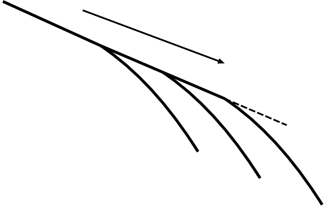
Figure 14: Self-Similar Evolution.

where $r_{00}$, $\rho_{00}$, $M_{00}$ are constants and $n$ is the power-law index of the cusp given by $\rho\propto r^{n}$. This self-similarity is illustrated in Figure 14. If we set $n=-1.5$ from the simulations, we obtain

$$\rho_{\dagger}(M) \propto M^{-1}$$ (8)

$$r_{\dagger}(M) \propto M^{2\over 3}.$$ (9)

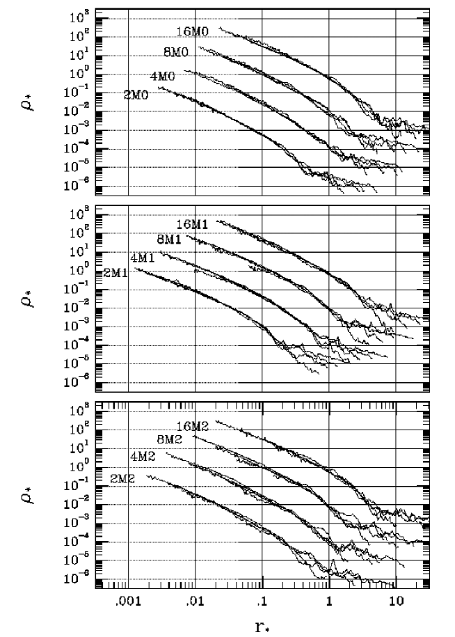
Figure 15: Self-similar evolution of the density profile. The scaled densities $\rho_{\ast}$ are plotted as a function of the scaled radius $r_{\ast}$. The profiles for Run 8M{0,1,2}, 4M{0,1,2} and 2M{0,1,2} are vertically shifted downward by 0.5, 1, 1.5 dex and horizontally shifted to the left by 0.5, 1, 1.5 dex, respectively.

In Figure 15, we plot $\rho_{\ast}$ defined through equations (4)-(7) as a function of $r_{\ast}$ Here, we took $M_{00}=10^{14}M_{\odot}$, $r_{00}=0.2$ Mpc, and $\rho_{00}=7\times 10^{-4}M_{\odot}/$pc³. We plot four density profiles at different values of the redshift $z$. We set $n=-1.5$ for all runs and use $M_{200}$ as the total mass. In this figure, we can see that the density profiles of the same halo at different times show very good agreement to each other, which means the density structure evolves self-similarly, though in outer region a degree of overlapping becomes worse. Therefore, Figure 15 demonstrates that our assumption of the self-similarity is justified.

3.5 Universality

In this subsection we discuss the universality of the density profile. Using a non-dimensional free parameter $\delta$, we define new non-dimensional variables expressed as

$$\rho_{\ast\ast} = \rho_{\ast}\delta^{-1}$$ (10)

$$r_{\ast\ast} = r_{\ast}\delta^{1\over 3}$$ (11)

Figure 16 shows $\rho_{\ast\ast}$ $r_{\ast\ast}$ of all Runs at $z=z_{\rm end}$. The values of $\delta^{-1}$ are 1.0, 0.4, and 0.6 for Run 16M{0,1,2}, 2.5, 1.0 and 3.0 for Run 8M{0,1,2}, 10.0, 3.0 and 6.0 for Run 4M{0,1,2}, and 35.0, 12.0 and 30.0 for Run 2M{0,1,2}. We can see that the 12 density structures agree very nicely, which means they are universal. In principle, any scaling on the $r$-$\rho$ plane can be expressed using two parameters. We used the total mass $M$ as one of two parameters to express the self-similarity discussed in section 3.4. The parameter $\delta$ corresponds to the other freedom. The value of $\delta$ is considered to reflect an amplitude of the density fluctuation at the collapse.

We attempted to fit the density structure to several profiles proposed in earlier studies. Figure 18 and 18 show the profile proposed by Moore et al. (1999) and by NFW. The function forms are given by $\rho_{\ast\ast}=r_{\ast\ast}^{-1.5}(1+r_{\ast\ast}^{1.5})^{-1}$ and by $\rho_{\ast\ast}=10(0.5r_{\ast\ast})^{-1}(1+0.5r_{\ast\ast})^{-2}$, respectively. Our simulation results agree with the profile proposed by Moore et al.(1999) very well, while the agreement with the NFW profile is not so good.

In summary, the density structure of simulated halos is well expressed by

$${\rho(r)\over\rho_{0}}(=\rho_{\ast\ast})=\displaystyle{1\over(r/r_{0})^{1.5}[1+(r/r_{0})^{1.5}]}\left(=\displaystyle{1\over r_{\ast\ast}^{1.5}[1+r_{\ast\ast}^{1.5}]}\right)$$ (12)

where

$$\rho_{0} = 7\times 10^{-4}\cdot\delta\displaystyle\left({M\over 10^{14}M_{\odot}}\right)^{-1}\quad(M_{\odot}{\rm/pc^{3}})$$ (13)

$$r_{0} = 0.2\cdot\delta^{-{1\over 3}}\displaystyle\left({M\over 10^{14}M_{\odot}}\right)^{2\over 3}\quad({\rm Mpc})$$ (14)

where again $M$ is the total mass of halos, $\delta$ is a non-dimensional free parameter. The free parameter $\delta$ is constant during evolution of a halo.

3.6 Formation Process of The Central Cusp

In this subsection, we show that the central cusp grows through the accretion of the disrupted smaller halos by a larger halo. In the bottom-up structure formation a typical halo grows through repeated merging of smaller halos. In the CDM hierarchical clustering, the larger halo typically has a denser central region than the smaller halo has. Therefore, the smaller halo is disrupted by the tidal field of the larger halo and the matter from the smaller halo is scattered around, when two halos merge. On the other hand, the central region of the larger halo survives the merging process more or less intact.

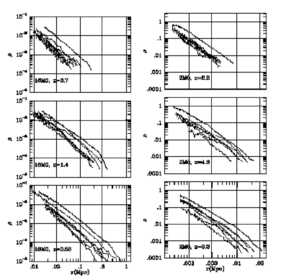
Figure 19: Density profiles of smaller halos which are going to merge to the larger halo. The thick curve indicates the larger halo.

In Figure 13, we can clearly see that the cusp grows outward without changing the inner part. In Figure 19 we show density profiles of halos which will merge to the largest halo, for Runs 16M0 and 2M0. We plot 6 halos with more than 1000 particles which are nearest from the potential minimum, together with the largest halo. It is clear that the central halo has the highest density.

The reason why larger halos have higher density can be understood as follows. Let us consider the peaks of the fluctuation whose characteristic scale is $\lambda$. If the total density field is only composed of the fluctuation whose scale is $\lambda$, the peaks will collapse to halos with similar density almost simultaneously. Actually, there are contributions from fluctuations whose scale is larger than $\lambda$, too. A peak in high-density background would collapse to a halo with higher density than peaks in low-density background, simply because of the difference in the background density. Later, the ”background”, which is just a density peak of longer wavelength, would collapse. During this collapse, however, the high-density peak collapsed earlier is not affected. Therefore, larger halo tend to have higher central density than smaller halos.

In Figure 20 we show one-dimensional trajectory of the particles for Run 16M0. We randomly select 10 particles from the particles whose distances from the center of the halo at the end of the simulation are 0.02-0.03, 0.1-0.2, and 1-2 Mpc Figure 20 shows that a large fraction of particles in the inner region settles there early, and those in the outer region tend to fall later. In other words, Figure 20 shows that the formation process discussed in the above actually takes place.

The cusp with the slope of $-1.5$ seems to be a ”fixed point” or a ”convergence point” for the growth of the halo through accretion of diffuse and small halos. Once the cusp with the slope of $-1.5$ forms, the density in the $r^{-1.5}$ cusp remains unchanged and the disrupted matter is accreted outside the $r^{-1.5}$ cusp, which is clearly shown in Figure 13.

Moreover, the power index of $-1.5$ seems to be a universal feature independent of the form of initial power spectrum. The high-resolution simulations presented in this paper and those by Moore et al. (1999) show that the power of the cusp is $-1.5$, independent of the mass scale. A preliminary result of our another simulation from the initial power spectrum of $P(k)\propto k^{-1.7}$, which is shallower than that at cluster scale for standard CDM model, also show that the power of the cusp is around $-1.5$.

Currently, we do not have a clear explanation why the slope of the cusp is $-1.5$ when it forms through the accretion of disrupted small halos. We will discuss this topic more comprehensively elsewhere.

3.7 Origin of The Outer Profile

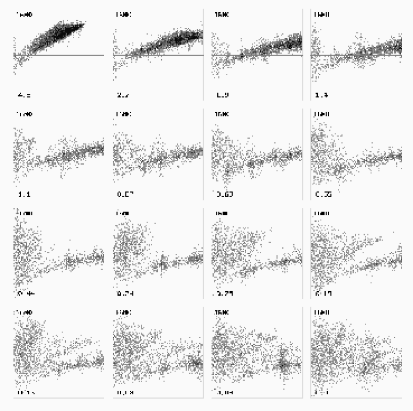
Figure 21: Distribution of particle in $r-v_{\rm r}$ plane at 16 different redshifts for $N$-body simulation Run 16M0. The number at lower-left corner of each panel indicates the redshift. The width of each panel is equal to $2r_{200}$ at $z_{\rm end}$. The range of radial velocity is from $-2031$ km/s to $2031$ km/s.

Figure 21 shows the distribution of particles on the $r$-$v_{\rm r}$ plane, where $r$ is distance from the center and $v_{\rm r}$ is the radial velocity, at 16 different redshifts for Run 16M0. We can see that the outer region consists of two component. The first component is infalling matters which is visible as thick stream of particles in the right-lower region of each panels. The vertical spreads visible in this stream are infalling smaller halos. The second component is the more scattered particles with nearly zero average velocity. As one can see from the time evolution, these stars gained energy in the central region when small halos accreted on the central halo. In Figure 22 we show density profiles of scattered and infalling particles separately. We separated two components by defining appropriate boundary in Figure 21. At around $r_{200}$, contribution of two components to the total profile are of the same order.

The profile in the outer region exhibits large fluctuations. The merging events occur intermittently, and the amount of scattered matter depends on earlier merging events. Nevertheless, the density profile fits the profile which is asymptotically proportional to $r^{-3}$, as shown in the previous section.

Consequently, in the outer region orbits of particles shows strong radial anisotropy. Figure 23 shows anisotropy in velocity distribution of the profile together with simulation results for Run 16M{0,1,2} and 2M{0,1,2}. The anisotropy are expressed by the anisotropy parameter $\beta$, defined as

$$\beta=1-{\langle v_{\theta}^{2}\rangle\over\langle v^{2}_{\rm r}\rangle},$$ (15)

where $\langle v_{\theta}^{2}\rangle$ and $\langle v^{2}_{\rm r}\rangle$ are mean tangential and radial velocity dispersion. In this definition, $\beta=0$ means the velocity distribution is isotropic and $\beta=1$ means completely radial.

4 Conclusion

We performed $N$-body simulations of dark matter halo formation in the standard CDM model. We simulates 12 halos whose mass range is $6.6\times 10^{11}M_{\odot}$ to $8.0\times 10^{14}M_{\odot}$. We introduced the accuracy criteria to guarantee that numerical artifact due to the two-body relaxation and the time integration do not affect the result, and obtained the density profile which is free from numerical artifact down to the radii $(0.01-0.02)r_{200}$.

Our main conclusions are:

• In all runs, the final halos have density cusps proportional to $r^{-1.5}$.

• The density profile evolves self-similarly.

• The density profile is universal, independent of the halo mass, initial random realization of density fluctuation and the redshift. The density structure is in good agreement with the profile proposed by Moore et al. (1999).

• We found that the central cusp grows through the disruption and accretion process of diffuse smaller halos. The slope of the central cusp seems to be a fixed point for the growth of the halo through accretion of tidally disrupted matter.

5 Discussion

Here we discuss the relation between our results and those of the previous studies.

We obtained steeper inner cusp than that obtained by NFW, which was already found in high-resolution simulations (FM97, Moore et al 1999, Ghigna et al.2000, Jing and Suto 2000). The reason for this disagreement is that in low-resolution simulations the central cusp is smoothed out by the two-body relaxation. If the cusp is shallower than $-2$, the velocity dispersion decreases inward. The energy flows inward due to the two-body relaxation and the central region expands, which is called the gravothermal expansion (Hachisu et al. 1978, Quinlan 1996, Heggie, Inagaki, McMillan 1994, Endo, Fukushige, Makino 1997). Therefore, the density in the cusp decreases and the cusp becomes shallower. Using the relations $t_{\rm rel}\sim v^{3}/(\rho m)$, $\rho\sim r^{-1.5}$, and $v\sim r^{0.25}$ and our simulation results, we can estimate the lower limit of the radius where the structure is free from the two-body relaxation effect as $\sim 0.01r_{200}(N/10^{6})^{-0.44}(\rho_{0}/2.7\times 10^{-4}M_{\odot}/{\rm pc}^{3})^{0.44}(\sigma_{0}/1300{\rm km/s})^{-1.33}$ for a cluster-sized halo at the present epoch, where $\sigma_{0}$ is velocity dispersion at the scale radius $r_{0}$. For simulations with $N=10^{4}$ and $10^{5}$ within $r_{200}$, the limits are estimated as $\sim 0.08r_{200}$ and $\sim 0.03r_{200}$, respectively. Therefore, simulations with $\sim 20$k particles the central cusp would be become significantly shallower due to relaxation.

We could not reproduce the dependence of the slope observed by Jing and Suto (2000). The difference could be also due to the smoothing by two-body relaxation in their cluster-sized halos. In this paper, we show that the density profile within $\sim 0.01r_{200}$ smoothed by the two-body relaxation. The density at $0.01r_{200}$ and the mass resolution in their cluster-sized halo are similar to those in ours. The density profile in their simulations within $0.01r_{200}$, at which the profile begins to depart from $r^{-1.5}$ inward, could be affected by the two-body relaxation.

Our result is in good agreement with results of simulations by Moore et al. (1999), in which the tidal field was included. This agreement suggests that the neglect of the tidal field in our present study and in FM97 hardly affects the density profile. The formation mechanism we discussed in this paper also suggests that the tidal field due to the mass outside the simulation sphere is not crucial.

Moore et al. (1999) argued that the merging process is not related with the structure. They simulated the halo formation using a power spectrum with a cutoff to suppress merging event in smaller scale and showed the profile does not change. However, in this simulation, several merging event took place since the cutoff wave length is rather short. Therefore, their conclusion that merging is not important is not really supported by their simulation. According to our explanation, several merging events where the central large halo swallows smaller halos determines the structure of the halo. Such events did took place in Moore et al.’s simulations.

As discussed in the Introduction, there are a lot of analytical and semi-analytical studies to explain the density structure. However, no study succeeded to explain the universality satisfactory. This is because none of them is based on the formation and growth process of the halo as discussed in this paper. Syer and White (1998) discussed that the cusp is a convergence point of disrupting and sinking of satellite, and that the convergence slope depends on the initial power spectrum. In their model, some of smaller halos were assumed to sink down to the center of the larger halo, when two halos merged. However, as we discussed, smaller halos are always disrupted and never sink down to the center, because the smaller halo is always less dense. Evans and Collet (1997) argued the cusp is a steady-state solution of Fokker-Plank equation. The solution is derived by assuming that many small clumps within a large halo evolve by the two-body relaxation. In our simulations, there are no such small clumps, since they are disrupted before they reaches the center.

Figure 3: Averaged density profiles for Run 16M0 and the same model as Run 16M0 but with $N$/4, $N$/16, and $N$/16 and 4$\varepsilon$, where $N$ and $\varepsilon$ are the number of particles and softening parameter for Run 16M0. The model with 4$\varepsilon$ is plotted in the dashed line. The unit of density is $M_{\odot}$/pc³.

Figure 4: The ratio of the averaged density for the same models as Fig 4 to that for the reference run (Run 16M0).

Figure 5: Same as Figure 4, but as a function of the ratio of the local relaxation time to the simulation period, $t_{\rm re}(r)/t$. The arrow indicates the accuracy criterion 3.

Figure 6: Averaged density profile for Run 16M0 in the thick line and the same model as Run 16M0 but with 4, 8, and 16 times larger and 4 times smaller time stepsize in the thin line. The unit of density is $M_{\odot}$/pc³.

Figure 7: The ratio of the averaged density for the same model as Fig 6 for the reference run (Run 16M0).

Figure 8: Same as Figure 8, but as a function of the ratio of the local dynamical time to time step size, $t_{\rm dy}(r)/\Delta t$. The arrow indicates the accuracy criterion 40.

Figure 9: Averaged density profiles for Run 16M0 ($\varepsilon=0.56$kpc) and the same model as Run 16M0 with $\varepsilon=$0.18, 1.7, 5, 15, 30 kpc, where $\varepsilon$ is the softening length. The unit of density is $M_{\odot}$/pc³. The numbers beside the lines indicates the softening length. The profiles for Run 16M0 and the models with $\varepsilon=1.7$kpc are plotted in the thick lines. The dashed lines indicates the density profile proportional to $r^{-1.5}$. The arrow indicates the critical radius defined by the accuracy criteria (1) and (2).

Figure 10: Evolution of density profile of the halo for Run 16M0. The unit of density is $M_{\odot}$/pc³. The profiles are vertically shifted downward by $7,6,...,1,0$ dex from the bottom to the top. The arrows indicates $r_{200}$. The numbers near the dashed lines indicate the power index of those lines. The numbers on the left of the profiles indicate the redshift.

Figure 11: Same as Figure 10, but for Run 2M0.

Figure 12: Density profile of the halo for all Runs at $z_{\rm end}$. The unit of density is $M_{\odot}$/pc³. The profile for Run 16M{0,1,2}, 8M{0,1,2}, and 4M{0,1,2} are vertically shifted upward by $1.5$, $1$, $0.5$ dex, respectively. The arrows indicate $r_{200}$. The thin solid and dashed lines indicate the densities proportional to $r^{-1.5}$ and $r^{-1}$.

Figure 13: Evolution of the density profile of the halo for Runs 16M0 and 2M0 with no vertical shift. The unit of density is $M_{\odot}$/pc³.

Figure 16: Universality in the density structure. The scaled densities $\rho_{\ast\ast}$ are plotted as a function of the scaled radius $r_{\ast\ast}$.

Figure 17: Fitting of the density structure by the profile proposed by Moore et al. (1999) (solid curve). The dashed line indicates $\rho\propto r^{-1.5}$.

Figure 18: Fitting of the density structure by the profile proposed by Navarro, Frenk, White (1996,1997).

Figure 20: One-dimensional trajectories of randomly selected 10 particles for Run 16M0. The distance from the center of halo is plotted as a function of time, together with the density profile at $z_{\rm end}$. The region indicated by thick curve in density profile indicates where the selected particles exists at $z_{\rm end}$.

Figure 22: Density profile of the halo for Run 16M0 as a superposition of two components. The dashed curves indicate that for the infalling matter and the thick curves indicate the scattered matter. The thin curve is total profile.

Figure 23: Anisotropy parameter, $\beta=1-v^{2}_{\theta}/v_{\rm r}^{2}$ as a function of radius at $z=z_{\rm end}$ for Runs 16M{0,1,2}(solid curve) and 2M{0,1,2} (dashed curves). The star, square, and triangle symbol indicate $\beta$ for {16,2}M0, {16,2}M1, and {16,2}M2, respectively.

References

- (1)
- (2) Avila-Reese, V., Firmani, C., Hernandez, X. 1998, ApJ, 505, 37
- (3)
- (4) Barnes, J. E. 1990, J. Comp. Phys., 87, 161
- (5)
- (6) Barnes, J. E., & Hut, P. 1986, Nature, 824, 446
- (7)
- (8) Bertschinger, E. 1998, ARA&A, 36, 599
- (9)
- (10) Brainerd, T. G., Goldberg, D. M., & Villumsen, J. V. 1998, ApJ, 502, 505.
- (11)
- (12) Bullock, J. S., Kolatt, T. S., Sigad, Y., Somervill, R. S., Kravtsov, A. V., Klypin, A., Primack, J. P., & Dekel, A. 2000, MNRAS, submitted.
- (13)
- (14) Cole, S., & Lacy, C. 1996, MNRAS, 281, 716
- (15)
- (16) Dubinski, J., & Carlberg, R. 1991, ApJ, 278, 496
- (17)
- (18) Endo, H., Fukushige, T. & Makino, J. 1997, PASJ, 49, 345
- (19)
- (20) Evans, W. N., & Collet, J. L., 1997, ApJ, 480, L103
- (21)
- (22) Fukushige, T., & Makino, J. 1997, ApJ, 477, L9
- (23)
- (24) Ghigna, S., Moore, B., Governato, F., Lake, G., Quinn, T., & Stadel, J. 2000, ApJ, submitted.
- (25)
- (26) Hachisu, I, Nakada, Y., Nomoto, K., Sugimoto, D. 1978, Prog. Theor. Phys. 60, 393
- (27)
- (28) Heggie, D. C., Inagaki, S., & McMillan, S. L. W. 1994, MNRAS 271, 706
- (29)
- (30) Heriksen, R. N., & Widrow, L. M. 1999, MNRAS, 302, 321
- (31)
- (32) Hernquist, L. 1990, ApJ, 356, 359
- (33)
- (34) Huss, A., Jain, B., & Steinmetz, M. 1999, ApJ, 517, 64
- (35)
- (36) Jing, Y. P. 2000, ApJ, 535, 30
- (37)
- (38) Jing, Y. P., & Suto, Y. 2000, ApJ, 529, L69
- (39)
- (40) Kawai, A., Fukushige, T., Makino, J., & Taiji, M. 2000, PASJ, 52, 659
- (41)
- (42) Kravtov, A. V., Klypin A. A., Bullock, J. S., Primack J. R., 1998, ApJ. 502, 48
- (43)
- (44) Kull, A. 1999, ApJ, 516, L5
- (45)
- (46) Lokas, E. L. 2000, MNRAS, 311, 423
- (47)
- (48) Makino, J. 1991, PASJ, 43, 621
- (49)
- (50) Moore, B., Governato, F., Quinn T., Statal, J., & Lake, G. 1998, ApJ, 499, L5
- (51)
- (52) Moore, B., Quinn T., Governato, F., Statal, J., & Lake, G. 1999, MNRAS, 310, 1147
- (53)
- (54) Navarro, J. F., Frenk, C. S., & White, S. D. M., 1996, ApJ, 462, 563
- (55)
- (56) Navarro, J. F., Frenk, C. S., & White, S. D. M., 1997, ApJ, 490, 493
- (57)
- (58) Nusser, A., & Sheth R., 1999, MNRAS, 303, 685
- (59)
- (60) Okamoto, T., & Habe, A. 1999, ApJ, 516, 591
- (61)
- (62) Quinlan, G, D., 1996, New Astronomy, 1, 255
- (63)
- (64) Spitzer, L., 1987,
- (65)
- (66) Steinmetz, M. H., & White, S. D. M., 1997, MNRAS, 288, 545
- (67)
- (68) Subramanian, K., Cen, R., & Ostriker, J. P. 2000, 538, 528
- (69)
- (70) Syer, D., & White, S. D. M., 1998, MNRAS, 293, 337
- (71)
- (72) Thomas, P. et al. 1998, MNRAS, 296, 1061
- (73)
- (74) Tormen, G., Bouchet, F. R., & White, S. D. M. 1996, MNRAS, 286, 865
- (75)
- (76) Yano, T. & Gouda, N. 2000, ApJ, 539, 493
- (77)