Evolution of highly buoyant thermals in a stratified layer

The buoyant rise of thermals (i.e. bubbles of enhanced entropy, but initially in pressure equilibrium) is investigated numerically in three dimensions for the case of an adiabatically stratified layer covering 6–9 pressure scale heights. It is found that these bubbles can travel to large heights before being braked by the excess pressure that builds up in order to drive the gas sideways in the head of the bubble. Until this happens, the momentum of the bubble grows as described by the time-integrated buoyancy force. This validates the simple theory of bubble dynamics whereby the mass entrainment of the bubble provides an effective braking force well before the bubble stops ascending. This is quantified by an entrainment parameter alpha which is calculated from the simulations and is found to be in good agreement with the experimental measurements. This work is discussed in the context of contact binaries whose secondaries could be subject to dissipative heating in the outermost layers.

1 Introduction

Highly buoyant bubbles with large specific entropy excess relative to the surroundings have been invoked by Hazlehurst (1985) in an attempt to explain the almost equal effective temperatures of the two components of contact binaries.

As noted by Sinjab et al. (1990) there are strong parallels between the highly buoyant bubbles of Hazlehurst and the ‘thermals’ found to occur in the earth’s atmosphere. Subsequently, Hazlehurst (1990) confirmed the existence of a formal relationship between Turner’s (1963) treatment of thermals, involving entrainment of matter, and his own treatment of highly buoyant bubbles (‘interlopers’) in contact binaries, as these bubbles annex new material.

In this paper we shall discuss the question of the validity, from a fluid-dynamical standpoint, of the simple bubble or thermal picture. We shall then go on to show how it is possible to determine numerically the value of the entrainment coefficient $\alpha$ (here called $\alpha_{\rm v}$) which enters Turner’s and several other investigations; the determination of a related coefficient (here called $\alpha_{\rm m}$) entering the Hazlehurst theory is also discussed.

We believe this to be the first attempt to evaluate the (previously semi-empirical) entrainment coefficient $\alpha$ on a fluid-dynamical basis.

2 Model setup

We adopt a basic setup of our model that is similar to that used normally to study convection in a stratified plane-parallel layer between impenetrable boundaries (e.g. Hurlburt et al. 1984). In particular, we use stress-free boundary conditions at the top and bottom, with a prescribed flux $F$ at the bottom and a prescribed temperature $T_{\rm top}$ at the top. Here, however, we assume the thermal equilibrium stratification to be adiabatic, so it is marginally stable to the onset of convection. Thus, when we insert a hot (buoyant) bubble, it will rise unaffected by the stratification (except for effects related to the growth and expansion of the ascending bubble), so there is no restoring force acting on the bubble as it rises.

2.1 Adiabatic stratification

Hydrostatic equilibrium requires that the weight of the atmosphere is balanced by the pressure gradient. However, if the entropy is constant, the pressure gradient can be written as $\rho^{-1}\mbox{\boldmath$\nabla$}{}p=\mbox{\boldmath$\nabla$}{}h$, where $p$ is pressure, $\rho$ is density, and $h$ is enthalpy. We adopt a perfect gas for which $h=c_{\rm p}T$, where $c_{\rm p}$ is the specific heat at constant pressure. For constant gravitational acceleration $g>0$, this implies a linear temperature stratification that is given by

$${{\rm d}{}\over{\rm d}{}z}(c_{\rm p}T)=g,$$ (1)

where $z$ is depth, which is assumed to increase downwards. Thus, the vertical temperature profile of the basic state is given by

$$T=T_{\rm top}+(z-z_{\rm top})g/c_{\rm p}.$$ (2)

In the absence of any motion there is only radiative flux, $F$, for which we adopt the diffusion approximation, so

$$\mbox{\boldmath$F$}{}=-K\mbox{\boldmath$\nabla$}{}T,$$ (3)

where $K$ is the radiative conductivity. Thermal equilibrium requires $\mbox{\boldmath$\nabla$}{}\cdot\mbox{\boldmath$F$}{}=0$, so the $z$-component of the flux is constant but, because the temperature gradient is constant, this is only possible if $K={\rm const}$. We now need to discuss the choice of $K$ and other parameters.

2.2 Choice of parameters

We adopt nondimensional units by defining a unit length $d$, and our bubble will usually have the initial radius $R_{0}=d$ (although we present initially some cases where $R_{0}=0.5\,d$. We measure time in units of $(d/g)^{1/2}$, density in units of $\rho_{0}$ (we choose $\rho=\rho_{0}$ at the location where the centre of the bubble will be introduced), and specific entropy, $s$, in units of $c_{\rm p}$. This corresponds to setting

$$d=g=\rho_{0}=c_{\rm p}=1.$$ (4)

A relevant nondimensional quantity is the normalised input flux

$${F\over\rho_{0}(gd)^{1/2}}\quad\mbox{(nondimensional input flux)}.$$ (5)

For secondaries of contact binaries this ratio is around $10^{-3}$. Specifying $F$ fixes $K=c_{\rm p}F/g$. There is however the numerical constraint that the mesh Peclet number, based on the sound speed $c_{\rm s}$ and the mesh width $\Delta x$,

$$\mbox{Pe}_{\rm grid}=\Delta x\,c_{\rm s}/\chi,$$ (6)

should not exceed a certain empirical upper limit of 10–100. This limit arises from the fact that the advection of sharp structures tends to generate small ripples on the scale of the mesh which need to be damped. Here, $c_{\rm s}^{2}=\gamma p/\rho$, $\gamma=c_{\rm p}/c_{\rm v}$ is the ratio of specific heats, and $\chi=K/\rho c_{\rm p}$ is the radiative diffusivity. In the present paper we shall consider values of $F$ in the range 0.001–0.005. In all cases we assume $\gamma=5/3$.

We adopt cartesian coordinates $(x,y,z)$ where $z$ points downwards. The bubble centre is placed initially at $x=y=z=0$. In order that the bubble be initially sufficiently far away from the bottom boundary and that it can rise over a distance of at least a few times its own radius (which is unity in most of the models), we chose the vertical extent of the computational box to be from $z_{\rm top}=-6$ to $z_{\rm bot}=2$.

Next, we fix the temperature stratification within the box by specifying the value of $T_{\rm top}$, which is held constant by the boundary condition chosen. The choice of this parameter is restricted by numerical considerations. Since temperature is proportional to the pressure scale height, small values of $T_{\rm top}$ imply a short pressure scale height at the surface. However, numerical stability and accuracy considerations require that the scale height cannot be less than at least 2–3 mesh zones. The non-dimensional pressure scale height at the top is

$$\xi_{0}=H_{\rm p,\,top}/d=(c_{\rm p}-c_{\rm v})T_{\rm top}/gd,$$ (7)

where we have included $d$ and $g$ factors, even though they are unity. For runs with $N_{z}=50$ meshpoints in the vertical direction, we were able to use $\xi_{0}=0.3$. For orientation, we note that this yields a $\ln(p_{\rm bot}/p_{\rm top})$ of 6.2 pressure scale heights between top and bottom of the box. The local pressure scale height at $z=0$ is then given by $0.4\times|z_{\rm top}|+\xi_{0}=2.7$. Using Eqs (2) and (7) we also see that the top of the adiabatic atmosphere would be at

$$z_{\infty}=z_{\rm top}-2.5\xi_{0}\quad\mbox{(for $\gamma=5/3$)},$$ (8)

but this should be outside the computational box. For $z_{\rm top}=-6$ and $\xi_{0}=0.3$ this gives $z_{\infty}=-6.75$.

For a perfect gas we have $p/\rho=(c_{\rm p}-c_{\rm v})T$ and $s=c_{\rm v}\ln p-c_{\rm p}\ln\rho$ (in dimensional form). The density stratification follows then from hydrostatic balance and the assumption that the entropy of the unperturbed model is constant:

$$\rho/\rho_{0}=(1-z/z_{\infty})^{1/(\gamma-1)}.$$ (9)

We mentioned already that we express density in units of $\rho_{0}$, which is the density at $z=0$, which is where the bubble will be positioned. Using this together with the definition of $s$ we can use Eq. (8) to express the value of the background entropy,

$$s_{0}=0.6\ln(-0.4z_{\infty})\quad\mbox{(for $\gamma=5/3$)}.$$ (10)

For $z_{\infty}=-6.75$ this gives $s_{0}=0.596$.

This completes the definition of the background state. We now turn to the discussion of the model equations and initial and boundary conditions adopted.

2.3 Governing equations

In the dynamical case the specific entropy is not only affected by the radiative flux divergence, but also by the rate of viscous dissipation, so

$$\rho T{{\rm D}\,{}s\over{\rm D}\,{}t}=\mbox{\boldmath$\nabla$}{}\cdot K\mbox{\boldmath$\nabla$}{}T+2\nu\rho\mbox{\boldmath${\sf S}$}{}^{2},$$ (11)

where ${\rm D}/{\rm D}t=\partial/\partial t+\mbox{\boldmath$u$}{}\cdot\mbox{\boldmath$\nabla$}{}$ is the lagrangian derivative, $\nu=\mbox{const}$ is the kinematic viscosity and

$${\sf S}_{ij}={\textstyle{1\over 2}}(\partial_{j}u_{i}+\partial_{i}u_{j}-{\textstyle{2\over 3}}\delta_{ij}\partial_{k}u_{k})$$ (12)

is the (traceless) rate of strain tensor. Equation (11) is solved together with the momentum equation,

$${{\rm D}\,{}\mbox{\boldmath$u$}{}\over{\rm D}\,{}t}=-{1\over\rho}\mbox{\boldmath$\nabla$}{}p+\mbox{\boldmath$g$}{}+{1\over\rho}\mbox{\boldmath$\nabla$}{}\cdot(2\nu\rho\mbox{\boldmath${\sf S}$}{}),$$ (13)

and the continuity equation

$${{\rm D}\,{}\ln\rho\over{\rm D}\,{}t}=-\mbox{\boldmath$\nabla$}{}\cdot\mbox{\boldmath$u$}{}.$$ (14)

We solve Eqs (11), (13) and (14) using the sixth order compact derivative scheme of Lele (1992) and a third order Hyman scheme for the time step. For earlier applications of this code see Nordlund & Stein (1990) and Brandenburg et al. (1996).

The value of $\nu$ is dictated again by numerical considerations, and in practice we take $\nu\approx\chi$, but note that $\nu$ is independent of $z$ whilst $\chi$ is not. In all cases considered below we have used $\nu=6\times 10^{-3}$.

2.4 Initial and boundary conditions

The bubble centre is placed initially at $x=y=z=0$ and has an entropy profile of the form

$$s=s_{0}+\Delta s\,\Phi(r),$$ (15)

where

$$\Phi(r)=\left\{\begin{array}[]{ll}\exp\left(-\displaystyle{{r^{2}\over R_{0}^{2}-r^{2}}}\right)&\quad\mbox{if $r<R_{0}$}\\ 0&\quad\mbox{otherwise}\end{array}\right.$$ (18)

is a profile function defining the initial shape of the bubble. Here $r$ is the initial distance from the centre. Initial pressure equilibrium requires that the increase of $s$ is compensated by a corresponding decrease of $\ln\rho$, so

$$\ln\rho={1\over\gamma-1}\ln\left(1-{z\over z_{\infty}}\right)-\Delta s\,\Phi(r).$$ (19)

The initial entropy excess of the bubble is given by the parameter $\Delta s$. [In all cases presented we take $\Delta s=0.5$, which corresponds to the value used by Hazlehurst (1985), who adopts units where the nondimensional specific entropy is larger by a factor of 5. We note that larger values of $\Delta s$ make the bubble rise faster, but we found that even for $\Delta s=2$ the motion remained subsonic.]

We assume stress-free boundaries at the top and bottom, and prescribe the value of $T$ at the top and $\partial T/\partial z$ at the bottom, as is usual for convection calculations (e.g. Hurlburt et al. 1984). We use periodic boundary conditions in the $x$ and $y$ directions. The horizontal extent of the box, $|x|<L_{x}$ and $|y|<L_{y}$, is varied between $L_{x}=L_{y}=4$ and 16.

2.5 Allowing for three-dimensional effects

In order to assess the fragility of the bubble during its ascent we have adopted in many cases substantial initial velocity perturbations. In Fig. 1 we show a three-dimensional representation of the entropy for a run with $\Delta s=0.5$ using initial velocity perturbations with $u_{\max}/c_{\rm s}=0.4$ and $u_{\rm rms}/c_{\rm s}=0.02$. As is evident from Fig. 1, the entropy of the blob is hardly affected by these perturbations and only near the surface does one see strong perturbations.

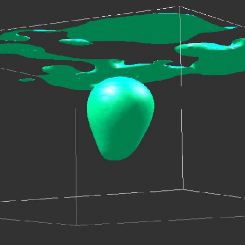
Figure 1: Three-dimensional representation of the specific entropy. The initial velocity perturbations are noticeable mostly near the top layers, but the bubble itself remains fairly axisymmetric. $100\times 100\times 50$ meshpoints.

It is interesting that the bubble remains an entity during much of its ascent. In fact, even when the initial condition is quite different, bubble-like structures tend to develop. As an example we show in Fig. 2 a case where we have introduced an almost uniform horizontal layer of enhanced specific entropy with a gaussian vertical profile initially. We have superimposed random small scale perturbations to get the buoyancy instability started.

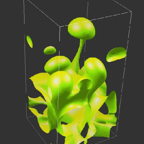
Figure 2: As Fig. 1, but for the case of a horizontal layer of enhanced specific entropy initially. $50\times 50\times 100$ meshpoints.

In the following we study in more detail the dynamics of an isolated buoyant bubble or thermal, as it shall also be referred to.

3 Dynamics of isolated thermals

In the following we consider cases with different degrees of stratification and different extents of the computational domain.

3.1 Modest stratification

We begin by considering first vertical cross-sections of entropy and velocity; see Fig. 3. The archimedian buoyancy force is largest in the middle of the bubble, and that is also where the vertical velocity is largest. On both sides of the bubble the velocity turns over, as expected (compare with observations of thermals described by Scorer 1957).

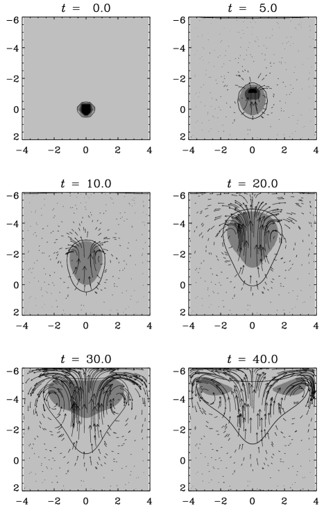
Figure 3: Velocity vectors superimposed on a grey scale representation of the entropy (dark indicates high entropy; all panels have the same grey scale). The velocity is shown in a fixed frame of reference. The initial specific entropy excess of the bubble is $\Delta s=0.5$ and its initial radius is $R_{0}=0.5$. The single contour shows the position where $s=s_{\rm crit}=0.001+s_{0}$. $F=0.005$, $50^{3}$ meshpoints.

A rather different impression is obtained when looking at the bubble in a comoving frame of reference; see Fig. 4. In this frame there is a stagnation point and hence there is a clear distinction of regions inside and outside the bubble. The flow pattern generally conforms with the notion of bubbles behaving like balloons with a more-or-less well defined surface and gas flowing around this surface. However, the bubble clearly grows in size and even its mass grows during its ascent.

It should be noted that this addition of new material with ‘different’ specific entropy does not contradict the bubble concept. This is because there is no entropy discontinuity between the bubble and the surroundings, so that the entropy of a captured particle can be changed gradually – by friction and by thermal diffusion – as it enters the bubble.

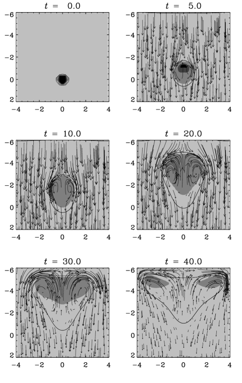
Figure 4: Same as Fig. 3, but now the velocity vectors are shown in a comoving frame of reference.

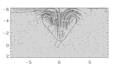
Figure 5: Same as Fig. 3, but for $t=30$ and for a wider box ($L_{x}=8$). Although in this calculation strong three-dimensional perturbations have been applied initially, the effects on the shape of the bubble are negligible. $F=0.005$, $100\times 100\times 50$ meshpoints, $\Delta s=0.5$, $R_{0}=0.5$.

By the time $t=30$ the effects of the lateral boundaries have begun to affect the evolution of the bubble. Therefore we show in Fig. 5 the case of a wider box ($L_{x}=8$). Note that there is now a noticeable flow speed even beyond $|x|=4$ (the extent of the box in the previous case). In this calculation we have also included strong velocity perturbations, but the overall flow pattern is still dominated by the rising bubble.

In order to quantify the rise and the growth of the bubble in detail, we define the bubble $B$ as all points in space where $s\geq s_{\rm crit}$, with $s_{\rm crit}$ just a little larger than the background value, which is here $s_{0}=0.596$, so we chose $s_{\rm crit}=0.597$. The volume of the bubble is then estimated as

$$V(t)=\int_{B}dV,$$ (20)

and the volume radius of the bubble is

$$R(t)=\left(V/{\textstyle{4\over 3}}\pi\right)^{1/3}.$$ (21)

The mass of the bubble is

$$M(t)=\int_{B}\rho\,dV.$$ (22)

In Fig. 6 we plot $R(t)$ and $M(t)$. Both functions increase monotonically, except for some minor departures at late times when the bubble has reached the top of the layer. Note also that at early times ($t<4$) $R$ increases somewhat faster than at later times. Qualitatively this type of behaviour is expected, because radiative diffusion causes structures to grow proportional to $t^{1/2}$, which causes an infinite slope of $R(t)$ at $t=0$.

Figure 6: Radius and mass of the bubble shown in Fig. 3. $F=0.005$, $50^{3}$ meshpoints, $\Delta s=0.5$, $R_{0}=0.5$.

In order to make further comparison with Hazlehurst’s theory of buoyant bubbles, we measure the position of the centre of mass of the bubble,

$$z_{\rm bubble}=\left.\int_{B}z\rho\,dV\right/\int_{B}\rho\,dV.$$ (23)

Since $z$ decreases upwards we define the height of the bubble as $h=-z_{\rm bubble}$. The height $h$ and velocity $v={\rm d}{}h/{\rm d}{}t$ of the bubble are shown in Fig. 7. Note that the height seems to approach a maximum near $h=3.5$, so the centre of mass of the bubble does note quite reach the top of the box. (Below we shall show that for larger bubbles, $R_{0}=1$, the maximum height is even less, suggesting that this is at least partly a geometrical effect; we shall also see that the top of the bubble does reach the top of the box in all cases.)

Figure 7: Height and speed of the bubble shown in Fig. 3. $F=0.005$, $50^{3}$ meshpoints, $\Delta s=0.5$, $R_{0}=0.5$.

Figure 8: Momentum and integrated buoyancy force acting on the bubble shown in Fig. 3. $F=0.005$, $50^{3}$ meshpoints, $\Delta s=0.5$, $R_{0}=0.5$.

The momentum of the bubble, $Mv$, is plotted in Fig. 8 and compared with the time integrated buoyancy force,

$$\int_{0}^{t}(M_{\rm d}-M)g\,{\rm d}{}t,$$ (24)

where

$$M_{\rm d}(t)=\int_{B}\tilde{\rho}\,dV$$ (25)

is the mass of displaced material and $\tilde{\rho}$ is the density of the undisturbed medium. Between $t=5$ and 15 the momentum of the bubble is somewhat larger than expected from the buoyancy force. This discrepancy depends somewhat on the definition of the boundary of the bubble. However, more dramatic is the sudden loss of momentum of the bubble after $t\approx 20$, whilst the buoyancy force, as estimated by Eq. (24), continues to operate beyond this time.

There are at least two possible reasons for this sudden braking effect. One reason could be that the blob gets too close to the top and loses momentum simply because of pressure build-up between the bubble and the top boundary. A second possibility could be that the bubble loses momentum due to some genuine resistance mechanism, such as wave braking or viscous friction. However, the braking effect seen in the simulations is too sudden and too strong to be explained by any genuine braking mechanism. Thus, we now turn to the first possibility, of which we can distinguish two variants. It is possible that the pressure build-up near the top is either an artifact of the top boundary being impenetrable, or it could be simply a feature of strong density stratification which causes the bubble to expand rapidly sideways. In order to drive strong sideways motions there must naturally be a horizontal pressure gradient which would also act in the vertical direction and slow down the ascent. This mechanism is known in compressible convection as buoyancy braking (Hurlburt et al. 1984).

In order to clarify the nature of the additional braking effect seen in the simulations, we first compare with a simulation using a somewhat taller box to see whether or not the braking sets in later, as would be the case if the impenetrable top boundary was the reason for the braking effect. (In the following we use calculations where $R_{0}=1$.)

3.2 Moving the top boundary further away

With $\xi_{0}=0.3$ and $z_{\rm top}=-6.0$ we have $z_{\infty}=-6.75$, see Eq. (8), so we can move the top boundary upwards by no more than about 10%. In the following, we discuss a model with $z_{\rm top}=-6.5$, but otherwise the same stratification. This means that at the new boundary we have to change $\xi_{0}$ by $\Delta\xi=0.4\times\Delta z=0.2$, so we have to require $\xi_{0}=0.1$.

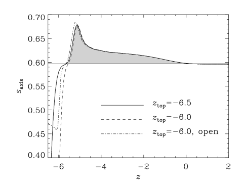
Figure 9: Vertical profile of $s$ along the axis of the bubble for $t=11$ and $z_{\rm top}=-6.5$ and $\xi_{0}=0.1$ (solid line) and $z_{\rm top}=-6.0$ and $\xi_{0}=0.3$ (dashed and dash-dotted lines for closed and open boundaries). Note that the entropy profile at the location of the bubble is not significantly affected by the value of $z_{\rm top}$. The region where $s>s_{\rm crit}$ is shown in grey. The entropy drop near the surface is a consequence of fixing the top temperature, but the location of this entropy drop moves further away as we extend the box. $F=0.001$, $50^{2}\times 100$ meshpoints, $R_{0}=1$.

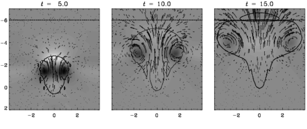
Figure 10: Grey scale representation of the pressure fluctuation together with velocity vectors and a contour marking the location where $s=s_{\rm crit}$. Light refers to high pressure fluctuation and dark to low pressure fluctuation. The surface at $z=-6$ is marked by a dash-dotted line. Above this line there is a zero-gravity ‘buffer layer’, modelling the effects of an open boundary.

In Fig. 9 we compare the vertical entropy profiles along the axis of the bubble for $z_{\rm top}=-6.5$ (with $\xi_{0}=0.1$) and $z_{\rm top}=-6.0$ (with $\xi_{0}=0.3$). We also compare with the case of an open top boundary that we have modelled by putting an extra layer on top of the box where gravity goes smoothly to zero and, as in Brandenburg et al. (1996), radiative diffusion is replaced by a heating/cooling term of the form $-\tau^{-1}(z)\rho(T-T_{\rm top})$, where $\tau^{-1}=0$ everywhere except above $z=z_{\rm top}$ where it goes smoothly to $\tau^{-1}=10$. This procedure allows the flow to penetrate the layer $z=z_{\rm top}$ freely.

It turns out that the entropy profiles at the location of the bubble are not significantly affected by the properties of the top boundary. The entropy drop near the surface is a consequence of fixing the top temperature, $T_{\rm top}$. Any increase in the logarithmic pressure at the top, $\delta\ln p_{\rm top}$, causes a corresponding decrease in the entropy, $\delta s_{\rm top}=-0.4\delta\ln p_{\rm top}$. Note, however, that the location of this entropy drop at the surface moves further away from the location of the bubble as we extend the box.

In Fig. 10 we show the pressure fluctuations (relative to the horizontal mean) together with velocity vectors. Near the top of the bubble there is a strong local maximum of the pressure fluctuation that drives the gas sideways. We have checked that the ram pressure integrated over the projected surface is roughly what is needed to explain the discrepancy between acceleration and buoyancy force. This is suggestive of buoyancy braking being the cause of the sudden drop of momentum seen in Fig. 8 (for $R_{0}=0.5$) and in Fig. 11 (for the present case of $R_{0}=1$).

In Fig. 11 we compare the evolution of $h$ in the two cases with different values of $z_{\rm top}$. Within the range of accuracy the two curves are consistent. Of course, the difference in the value of $z_{\rm top}$ is not very large, but the increase in the total number of scale heights covered in the simulation is significant: the value of $\ln(p_{\rm bot}/p_{\rm top})$ has increased from 6.2 to 9.0 pressure scale heights.

Figure 11: Height of the bubble (as measured by $h$, $h_{s}$ and $h_{\rm top}$) for different values of $z_{\rm top}$. Note that the top of the bubble, $h_{\rm top}$, reaches the top boundary. $F=0.001$, $50^{3}$ and $50^{2}\times 100$ meshpoints, $\Delta s=0.5$, $R_{0}=1$.

Note that $h$ reaches a maximum around $3$, i.e. significantly less than the value of $|z_{\rm top}|$. This is partly a geometrical effect, because smaller bubbles are able to travel somewhat further (in the previous subsection, where $R_{0}=0.5$ instead of 1.0, the bubble went to $h=3.5$). In the case of the open top boundary, the bubble rises till $h=4$, which is still small compared with $|z_{\rm top}|=6$. The relatively small values of $\max(h)$ are partly due to the fact that $h$ measures the position of the centre of mass, but in the strongly stratified case most of the mass is at the bottom of the bubble. Furthermore, in all cases considered the bubbles take mushroom form with a significant portion of the mass residing in the stem of the mushroom. A somewhat better representation of where most of the hot material resides is gained by looking at the value of the entropy weighted height, $h_{s}=-z_{s}$, where

$$z_{s}=\left.\int_{B}z(s-s_{\rm crit})\rho\,dV\right/\int_{B}(s-s_{\rm crit})\rho\,dV,$$ (26)

which is also plotted in Fig. 11. However, even the entropy weighted height of the bubble is not very close to the top of the bubble. Nevertheless, the location $h_{\rm top}$ of the top of the bubble, i.e. where $s=s_{\rm crit}$, does reach value close to $|z_{\rm top}|$; see Fig. 11. There remains however some worry that the centre of mass of the bubble is generally unable to travel great distances. In order to clarify this possibility we now consider the case of weak stratification where we can easily increase the extent of the box.

3.3 Weak stratification

We now consider a case of weak stratification and two different values of $z_{\rm top}$ ($-6$ and $-14$); hence we choose $\xi_{0}=30$ and $\xi_{0}=26.8$ respectively, so that the background stratification is the same for $-6<z<2$. The total number of pressure scale heights in these two cases is $\ln(p_{\rm bot}/p_{\rm top})=0.25$ and 0.5, respectively.

Figure 12: The effect of the vertical extent of a weakly stratified box on the balance between momentum and integrated buoyancy force acting on the bubble. $F=0.005$, $50^{3}$ and $50^{2}\times 100$ meshpoints, respectively. $\Delta s=0.5$, $R_{0}=1$.

In Fig. 12 we compare the momentum balance for the two cases with different values of $z_{\rm top}$. Again, the agreement between the momentum and the time integrated buoyancy force is good up to $t=10$ (for $z_{\rm top}=-6$) or up to $t=30$ (for $z_{\rm top}=-14$). The presence of the boundary clearly influences the motion of the bubble; nevertheless the top of the bubble does manage to reach the boundary, as we see from Fig. 13 (for weak initial perturbations) and Fig. 14 (for strong initial perturbations). This is in contrast to the results of Sinjab et al. (1990) who conclude that the blobs in their calculations ‘fail to reach the top of the envelope’. In our calculation the hot part of the bubble seems to stop at some point just below the boundary and stays there. Furthermore, Sinjab et al. (1990) interpret their two-dimensional calculations as indicating a fragmentation. We found no indication of any such effect, irrespective of whether the stratification was weak or strong. For comparison we also carry out two-dimensional cartesian calculations verifying that in the two-dimensional case the eddies do eventually travel downwards when they come sufficiently close to the horizontal boundaries. Again, in the weakly stratified case the bubbles can travel to large heights, but the effects of the boundaries begin to become important much earlier than in the three-dimensional case; see Fig. 15.

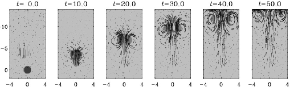
Figure 13: Velocity vectors superimposed on a grey scale representation of the entropy for a tall box with weak stratification. The velocity is shown in a fixed frame of reference. (The velocity vectors at $t=0$ at $z\approx-4$ result from the initial perturbation.) The initial specific entropy excess of the bubble is $\Delta s=0.5$ and its initial radius is $R_{0}=1.0$. $50^{2}\times 100$ meshpoints.

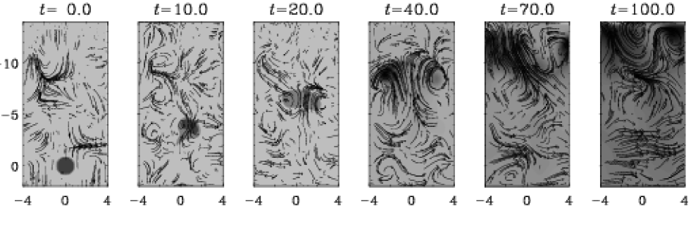
Figure 14: As for the run shown in Fig. 13, but with strong three-dimensional perturbations. For each time the grey scale is here adjusted between minimum and maximum values of $s$. Note that the bubble still makes it all the way to the top of the box, albeit at a somewhat later time.

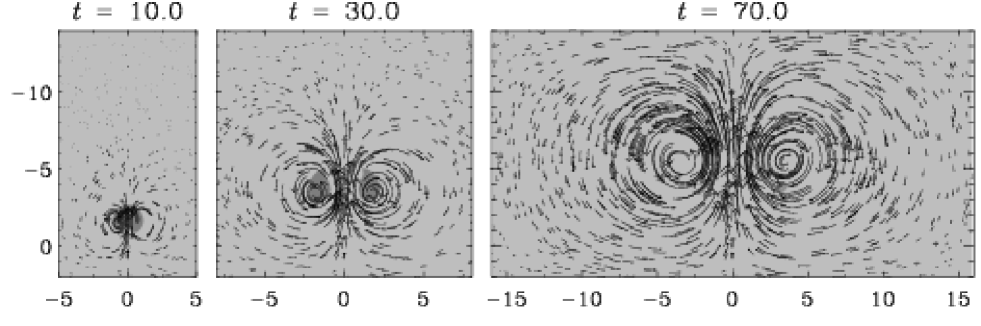
Figure 15: Velocity vectors superimposed on a grey scale representation of the entropy for the same case as in Fig. 13, but for a two-dimensional cartesian calculation. After $t=20-30$ the results begin to be affected by boundary effects. This is related to the strong nonlocality of two-dimensional calculations. Note that $L_{x}=16$, but in the first two panels only a smaller range is shown. $R_{0}=1.0$. $200\times 100$ meshpoints.

The results of Sinjab et al. (1990) are of course for the stratified case. However, our point is that it is the restriction to two dimensions (in cartesian geometry) that causes boundary effects to become extremely pronounced. Since stratification itself can also act as an effective boundary, it was necessary to go to the weakly stratified case where it is possible to move the boundaries much further away. Although the box shown in Fig. 15 was big enough to prevent the edge of the bubble from moving down again, boundary effects did begin to affect the evolution at times as early as $t=20$.

The ability of our bubble to rise right to the top of the box might seem surprising when one recalls that atmospheric thermals only manage to reach a certain maximum height. However one must not forget that the buoyancy force, relative to gravity, is here orders of magnitude greater than in the case of a typical atmospheric thermal (see e.g. Scorer 1957). A better analogy might therefore be that of an air bubble rising through water and eventually reaching the surface.

4 Calculation of the entrainment parameter

The introduction of a parameter to describe the entrainment of fluid by a rising ‘cloud’ was proposed by Morton et al. (1956). They introduced an equation of the form

$$\dot{V}=4\pi R^{2}\alpha_{\rm v}v,$$ (27)

which they regarded as describing ‘conservation of volume’. We have here rewritten their Eq. (16) using a slight change of notation. The ‘constant’ $\alpha_{\rm v}$ will be referred to hereafter as the volume entrainment coefficient. The above equation can be simplified to

$$\dot{R}=\alpha_{\rm v}v,$$ (28)

where $R$ is the volume radius.

We note that Eq. (27) is taken over in the work of Turner (1963), with $\alpha_{\rm v}$ becoming Turner’s ‘alpha’.

Now the concept of ‘conservation of volume’ lying behind Eq. (27) will be unfamiliar to many physicists. We therefore thought it to be worthwhile to concentrate instead on the accretion of mass rather than of volume and to write

$$\dot{M}=4\pi R^{2}\langle\tilde{\rho}\rangle\alpha_{\rm m}v,$$ (29)

where $\dot{M}$ is the mass entrainment rate, $\langle\tilde{\rho}\rangle$ some average of the surrounding material density near the bubble, and $\alpha_{\rm m}$ the mass entrainment coefficient. Although an average of $\tilde{\rho}$ over the bubble surface might be more appropriate, it is more convenient (and adequate for present purposes) to use a volume average. This gives

$$\dot{M}={3\over R}M_{\rm d}\alpha_{\rm m}v$$ (30)

where, as before, $M_{\rm d}$ is the mass displaced by the bubble.

We can now use Eqs (28) and (30) to calculate $\alpha_{\rm v}$ and $\alpha_{\rm m}$, all other quantities being already known. The results are shown in Figs 16 and 17.

Figure 16: Entrainment parameters $\alpha_{\rm m}$ (solid line) and $\alpha_{\rm v}$ (dashed line) for the case of strong stratification, $z_{\rm top}=-6.0$ and $\xi_{0}=0.3$, and two different initial bubble radii. In the upper panel, thick lines (solid and dashed) refer to the case with $z_{\rm top}=-6.5$ and $\xi_{0}=0.1$. Note that in the case of open boundaries (and $z_{\rm top}=-6.0$; upper panel) the value of $\alpha_{\rm m}$ remains at about 0.4 after $t=10$.

Figure 17: Entrainment parameters $\alpha_{\rm m}$ (solid line) and $\alpha_{\rm v}$ (dashed line) for the weakly stratified cases with $z_{\rm top}=-14$ ($\xi_{0}=26.8$) and $z_{\rm top}=-6$ ($\xi_{0}=30$). In the inset one sees more clearly that for $z_{\rm top}=-6$ there is still some indication of a plateau in $\alpha_{\rm m}$ and $\alpha_{\rm v}$. $R_{0}=1.0$.

It is interesting to note that for those parts of the curves not influenced by the special effects discussed previously, the quantity $\alpha_{\rm v}$ is in reasonable agreement with the experimental values of 0.25–0.34 (Morton et al. 1956, Turner 1963), with the agreement being better in the more strongly stratified case. For smaller initial bubble radii, $R_{0}=0.5$, $\alpha_{\rm v}$ attains noticeably larger values. Nevertheless, for both bubble radii investigated $\alpha_{\rm m}$ is roughly comparable ($\alpha_{\rm m}\approx 0.25$). Thus, the assumption of Turner (1963) that the value of $R_{0}$ does not influence ‘alpha’ can be verified only for $\alpha_{\rm m}$.

Better agreement between the ‘experimental’ and ‘calculated’ values cannot perhaps be expected since the Reynolds numbers for our calculations are lower than those appropriate to the experimental results, which leads to a more laminar entrainment process in our case.

Regarding $\alpha_{\rm m}$, we note that the entrainment of material leads to an effective drag force on the bubble given by

$$\mbox{Drag force}=\dot{M}v=4\pi R^{2}\tilde{\rho}\alpha_{\rm m}v^{2},$$ (31)

which may be compared with the normal hydrodynamic drag

$$\mbox{Hydrodynamic drag}={\textstyle{1\over 2}}\pi R^{2}\tilde{\rho}C_{\rm D}v^{2},$$ (32)

with $C_{\rm D}$ being the hydrodynamic drag coefficient. According to Moore (1967), normal hydrodynamic drag plays only a minor rôle in influencing the motion of a thermal. We can now check Moore’s point with the help of Eqs. (31) and (32); we confirm that hydrodynamic drag really does have only a minor influence on the motion, except possibly during the final stages in the weakly stratified case.

5 Details of the entrainment

Details of the entrainment process are viewed best in terms of tracer particles that are passively advected by the flow. In Fig. 18 we show the location of initially uniformly distributed particles at $t=10$. Particles that were originally inside the bubble (as defined by $s\geq s_{\rm crit}$) remain inside the bubble for all times. However, an increasing portion of new particles from outside the bubble is constantly being entrained, which happens mostly through the top boundary of the bubble. These particles then move along the periphery of the bubble tailwards where they find their way into the centre of the ring vortex associated with the bubble.

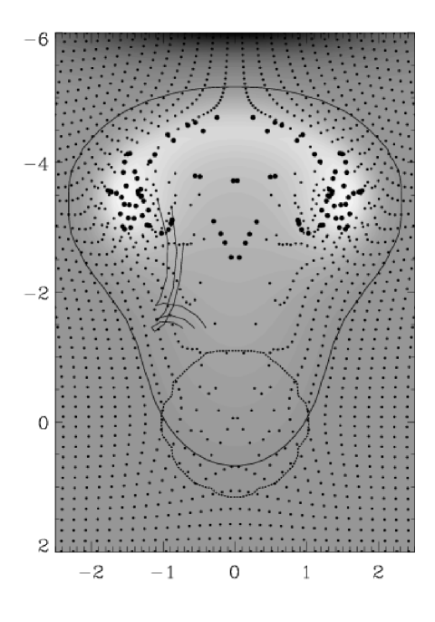
Figure 18: Tracer particles superimposed on a grey scale representation of entropy (bright indicates high entropy). Large dots represent particles for which initially $s\geq s_{\rm crit}$, i.e. which originated in the initial bubble. Small dots represent particles that come from outside the original bubble. The contours show the position where $s=s_{\rm crit}$ (dashed for the initial time and solid for $t=10$). The three neighbouring lines show the particle trajectory of entrained particles that were originally outside the bubble (at $x=-0.72$, to $-0.40$ and $z=-1.43$, and have now moved upwards to the point indicated by a small dot). Note that $L_{x}=4$, but only the range $|x|\leq 2.5$ is shown. $100^{2}\times 50$ meshpoints, $\Delta s=0.5$, $R_{0}=1.0$.

In Fig. 18 we have also indicated the trajectory of three neighbouring particles that were originally above the bubble and were subsequently entrained and lifted upwards together with the bubble. The kinks in each of these trajectories correspond to the moment at which the particles were overtaken by the bubble and became entrained.

6 Conclusions

The main aim of this paper was to test the validity of the bubble or thermal concept; in this respect the following conclusions can be drawn.

We found that the bubble could easily be followed as a well-defined entity throughout the calculations. Nevertheless, its dynamical behaviour consisted of two distinct phases. In the first of these, the dynamical behaviour expected from the simple bubble dynamics of equating buoyancy forces to rate of momentum change was indeed confirmed. However, in the second phase an unexpected braking effect appeared. Further investigation led us to attribute this effect to a combination of boundary effects (artificial) and buoyancy braking (real).

We found, in contrast to the results of Sinjab et al. (1990), that the top part of the bubble goes on rising until it reaches the surface. Bubbles penetrating to the surface layers favour the view that dissipation is an important factor in understanding contact binaries (Hazlehurst 1985, 1996).

Since the code used by us was a three-dimensional one including effects of viscosity and thermal (radiative) conductivity, we were in a position to follow in detail and more realistically the mass changes of the bubble due to entrainment of material. This made it possible for us to calculate the value of the entrainment coefficient $\alpha$ rather than, as was previously necessary, to take some value from glider observations (atmospheric thermals) or experiment. The values found by us were in good agreement with the those derived empirically, although the non-constancy of ‘alpha’ means that we have throughout referred to the entrainment coefficient rather than the entrainment constant. Finally, the introduction of a mass entrainment coefficient to replace (or at least supplement) the previously used volume coefficient appears to us desirable on physical grounds.

- (1) Brandenburg, A., Jennings, R. L., Nordlund, Å., Rieutord, M., Stein, R. F., Tuominen, I. 1996, JFM 306, 325
- (2) Hazlehurst, J. 1985, A&A 145, 25
- (3) Hazlehurst, J. 1990, MNRAS 247, 30p
- (4) Hazlehurst, J. 1996, A&A 313, 487
- (5) Hurlburt, N.E., Toomre, J., Massaguer, J.M. 1984, ApJ 282, 557
- (6) Lele, S. K. 92, J. Comput. Phys. 103, 16
- (7) Moore, D. W. 1967, in Aerodynamic Phenomena in Stellar Atmospheres, IAU Symposium 28, ed. R. N. Thomas (Academic Press, London and N.Y.), p.405
- (8) Morton, B. R., Taylor, G. I., & Turner, J. S. 1956, Proc. Roy. Soc. Lond. A 234, 1
- (9) Nordlund, Å., Stein, R. F. 1990, Comput. Phys. Commun. 59, 119
- (10) Scorer, R. S. 1957, JFM 2, 583
- (11) Sinjab, I. M., Robertson, J. A., Smith, R. C. 1990, MNRAS 244, 619
- (12) Turner, J. S. 1963, JFM 16, 1