On the Observational Characteristics of Inhomogeneous Cosmologies:
Undermining the Cosmological Principle
or
Have cosmologists put all their EGS in one basket?

A Ph.D. Thesis submitted to
The University of Glasgow.

Christopher A. Clarkson B.Sc.
December 1999

Astronomy and Astrophysics Group,
Department of Physics and Astronomy,
University of Glasgow,
Glasgow, G12 8QQ.
© C. A. Clarkson, 1999

The Cosmological Principle

Summary

This thesis concerns the compatibility of inhomogeneous cosmologies with our present understanding of the universe. It is a problem of some interest to find the class of all relativistic cosmological models which are capable of providing a reasonable ‘fit’ to the universe. One can imagine building up an (infinite-dimensional) parameter space containing all cosmological models. At any time the understanding of the universe would represent a blob in parameter space in which, presumably, the real universe would sit. This thesis, in some respects, is part of this process. We consider Stephani models, which are a generalisation of the standard Friedmann-Lemaître-Robertson-Walker (FLRW) models, which can be thought of as FLRW models with curvature which changes over time. This changing curvature reflects the existence of spatial pressure gradients which leads to an acceleration of the fundamental observers. Thus these models generalise the ‘dust’ assumption of standard cosmology.

Models normally considered in the ‘classification scheme’ approach are usually homogeneous dust or barotropic perfect fluid models. They are anisotropic however, and thus generalise the FLRW models. Most importantly, because these models are homogeneous, they satisfy the Copernican principle. The crucial aspect of this work is the retention of the Copernican principle – an assumption regarded by many as crucial to cosmology. It states that we are not at a special location in the universe. This is a vital aspect of the original work in this thesis: consideration of an inhomogeneous model, while retaining the Copernican principle has, as far as the author is aware, not been considered in detail before.

One may formulate the Copernican principle in many ways, from assuming we are not at a special location, to assuming that all (or most) locations are equivalent, which more or less forces homogeneity. Because the models considered here are inhomogeneous, they cannot satisfy the stronger version of the Copernican principle entirely – all locations will not be equivalent. However, we may demand that they are observationally indistinguishable. This is the tactic we use here. En route to this goal we must therefore calculate all observable quantities at any location in the spacetime. Certain properties of the Stephani models we consider allow us to do this exactly; consequently, many results of this thesis present, for the first time, observational relations for a class of inhomogeneous cosmological models which are exact, and valid for any observer position in the spacetime.

It may reasonably be claimed that the standard model is perfectly acceptable. However, a number of the properties of the models considered here do make them rather appealing. For example it is shown in §5.1 these models do not suffer from the horizon problem which is prevalent in the standard model. Also, the current conflict between cosmologists measuring a small but non-zero cosmological constant, and particle physics requiring it to be either zero or one hundred and twenty orders of magnitude higher, may be motivation in itself for considering cosmologies with a somewhat non-standard matter content.

In chapter 1 a brief review of the Copernican and cosmological principles in in homogeneous cosmologies is presented. A discussion is given of the present understanding of the important parameters of the standard model, some methods used to find these parameters, and some of the problems encountered.

In chapter 2 an overview of relativistic cosmology is presented. This is necessarily incomplete, with an emphasis on deriving observable relations, and on the FLRW models. The 1+3 formalism is presented. Some new results are presented concerning conformally related spacetimes (which turn out to be useful but not necessary for deriving the observational quantities in the Stephani models). FLRW models are then reviewed. We give a discussion of the generalised definitions of the Hubble constant and deceleration parameter in non-standard cosmologies.

In chapter 3 we discuss a theorem of fundamental importance to cosmology – the Ehlers-Geren-Sachs theorem (1968). This condition singles out spacetimes which will allow an isotropic cosmic microwave background (CMB). When applied to a dust universe it says that the existence of an isotropic CMB for every observer in the spacetime implies that the universe is FLRW. We extend this theorem to include the case of non-geodesic observers (in a perfect fluid model), which singles out a subclass of the Stephani models with symmetry. These models form the basis of the rest of the thesis. This chapter is a slightly extended version of Clarkson and Barrett (1999).

Chapter 4 takes the models which were singled out in chapter 3 and derives the observational relations for these models. Consideration is given to non-central observers, and the observational relations are then derived for any location in the spacetime.

The following two chapters examine the models in some detail from every observer position. The ‘worst case’ – ie, the observer position most restrictive on the parameter space – is singled out for each constraint, and it is shown that there is a large area of parameter space which is allowed by the tests we consider. In addition it is shown that some of the allowed models are distinctly inhomogeneous. Chapter 5 is the most thorough, and deals exclusively with the spherically symmetric subclass of the models derived in chapter 3.

Contents

1. 1 Introduction and Review
   1. 1.1 The FLRW Models
   2. 1.2 The Hubble constant
   3. 1.3 The Density Parameters $\Omega_{0}$ and $\Omega_{\Lambda}$, and the Curvature
   4. 1.4 Age
2. 2 Relativistic Cosmology
   1. 2.1 The Covariant 1+3 Formulation of Fluids in GR
      1. 2.1.1 Kinematics of the Fundamental Congruence
      2. 2.1.2 The Energy-Momentum Tensor
      3. 2.1.3 The Splitting of the Weyl Tensor
   2. 2.2 Splitting Einstein’s Equations
   3. 2.3 1+3 Splitting Under a Conformal Transformation
   4. 2.4 Relativistic Thermodynamics
   5. 2.5 Fluids in Cosmology
      1. 2.5.1 Perfect Fluids and Dust Models
      2. 2.5.2 Scalar Fields
      3. 2.5.3 Velocity Fields
      4. 2.5.4 More General Fluids
   6. 2.6 The CMB Anisotropies
   7. 2.7 Observations in the 1+3 Formalism
      1. 2.7.1 Observable Quantities From Discrete Sources
   8. 2.8 FLRW Models
      1. 2.8.1 The Magnitude-Redshift Relation
      2. 2.8.2 Observable Quantities in FLRW Models
   9. 2.9 Observable Quantities in a General Spacetime
3. 3 The Ehlers-Geren-Sachs Theorem and Some Generalisations
   1. 3.1 The Irrotational Perfect Fluid Solutions.
      1. 3.1.1 The Barnes Solutions.
      2. 3.1.2 The Conformally Flat Solutions
      3. 3.1.3 Symmetry and Thermodynamic Schemes.
   2. 3.2 QCDM Models.
   3. 3.3 Conclusions.
4. 4 Derivations of the Observational Relations
   1. 4.1 The Stephani Models Which Admit an Isotropic Radiation Field.
      1. 4.1.1 Geometry.
      2. 4.1.2 Non-Central Observers.
   2. 4.2 Observational Relations
      1. 4.2.1 Redshift
      2. 4.2.2 Distance-Redshift Relations
      3. 4.2.3 Number-Count-Redshift Relation
   3. 4.3 Discussion
5. 5 Observational Characteristics With $\zeta=0$
   1. 5.1 Lookback Time and the Horizon.
      1. 5.1.1 Matter Content and Energy Conditions.
   2. 5.2 Constraining the Model Parameters Using Observations.
      1. 5.2.1 Hubble’s Constant.
      2. 5.2.2 The Age of the Universe.
      3. 5.2.3 Size and the Distance-Redshift Relation.
      4. 5.2.4 The Microwave Background Anisotropy.
      5. 5.2.5 The Local Dipole Anisotropy
      6. 5.2.6 The Combined Exclusion Diagrams.
   3. 5.3 The Size of the Inhomogeneity.
   4. 5.4 Fitting to FLRW Models
   5. 5.5 Conclusions.
6. 6 Observational Characteristics When $\zeta\neq 0$
   1. 6.1 Hyperbolic Stephani Models: Overview
   2. 6.2 Energy Conditions
   3. 6.3 $H_{0}$
   4. 6.4 Age
   5. 6.5 Area Distance
   6. 6.6 The CMB Anisotropy
   7. 6.7 The Magnitude-Redshift Relation
   8. 6.8 Summary
7. 7 Conclusions and Future Work
   1. 7.1 A Note On ‘Best Fits’ and $a>0$
   2. 7.2 The Local Dipole
   3. 7.3 Almost EGS Considerations
   4. 7.4 Further Considerations
8. A Coordinate transformations and the Stephani Spacetimes.
9. B Transformation to a Non-Central Position.

List of Figures

1. 1.1 The variation in the accepted value of the cosmological constant over time, from Freedman (1999).
2. 1.2 The CMB multipoles as a function of temperature. From Max Tegmark’s home page: http://www.sns.ias.edu/~max/foregrounds.html.
3. 2.1 An observer measuring the area distance of a galaxy.
4. 2.2 Area distance as a function of redshift for a variety of ‘standard’ models. The closed model has $\{\Omega_{0},\Omega_{\Lambda_{0}}\}$=$\{0.3,1.5\}$, Einstein-de Sitter (1932) has $\{1,0\}$, flat: $\{0.3,0.7\}$ and the open model has $\{0.1,0\}$. All the models have $H_{0}=60$ km s^-1 Mpc^-1. Note that all the curves match up for low enough redshift.
5. 2.3 Coordinate distance as a function of redshift the models of figure 2.2.
6. 2.4 Apparent magnitude as a function of redshift for the models of figure 2.2
7. 2.5 The exact magnitude-redshift relation minus the same function as a power series relation to various orders. $|m_{{}_{\mathrm{e}xact}}-m_{{}_{\mathrm{s}eries}}|>0.1$ would give a significant detectable error.
8. 2.6 As in figure 2.5, but for the Stephani models considered later.
9. 2.7 The best fit to the $m(z)$ function for the supernovae data of Perlmutter et al., (1998b). the confidence regions do nothing for determining $\Omega_{0}$ and $\Omega_{\Lambda_{0}}$.
10. 2.8 The phase diagram for the $m-z$ relation for $z=0.5,5,1000$ presented in the $\Omega_{0}-\Omega_{\Lambda_{0}}$ plane. We can see that the contours move round the diagram with increasing redshift. The faint dashed lines are constant $q_{0}$, which shows that low redshift observations will give good results for $q_{0}$.
11. 2.9 A futureistic diagram of what might be expected from SNIa and CMB complementing each other in the future. The errors on $\Omega_{0}$ and $\Omega_{\Lambda_{0}}$ (small black ellipse) are extremely small (by cosmology standards) in comparison with the independent results. Plagiarised from Tegmark, Eisenstein and Hu (1998a).
12. 2.10 Extra results similar to (2.8) for other number-counts, age and growth as well. From Tegmark et al., (1998b).
13. 4.1 Stereographic projection of a sphere showing the relationship between the coordinates $r$ and $\chi$. Note that one can envisage the angle $\chi$ increasing steadily round the sphere ad infinitum.
14. 5.1 Lookback time and the past null cone on the Einstein cylinder. This shows the null structure for any model conformal to the Einstein static spacetime, including the Da̧browski and FLRW models. In FLRW models, the big bang occurs at $\eta=0$, whereas in Da̧browski models, the spacetime extends to $\eta=-\infty$.
15. 5.2 As in figure 5.1, but now using the actual Da̧browski model time coordinate, $t$.
16. 5.3 Surface plot of the proper age of the universe for $H_{0}=50$ km s^-1 Mpc^-1 with the observer at $\psi=\pi$.
17. 5.4 $\tau_{0}=12$ Gyr exclusion plot for different observer positions, for $H_{0}=60$ km s^-1 Mpc^-1. In the shaded areas the models are not old enough. $\psi=\pi$ is clearly the most restrictive case.
18. 5.5 The age exclusion diagram for various $H_{0}$ and proper age $\tau=10$ Gyr. The shaded region represents the prohibited area. Also shown as dashed lines are the age limits for $\tau=12$ Gyr. (Note that the region excluded for $H_{0}=70$ km s^-1 Mpc^-1 contains the excluded regions for lower $H_{0}$ – the progressively darker shading indicates this.)
19. 5.6 Area distance from the centre as a function of $\chi$ for two values of $b$. $T=15$ Gyr, $a=-1$.
20. 5.7 Area distance from the centre as a function of redshift for the same parameters as figure 5.6. For small $b$ the angular size distance oscillates far too rapidly.
21. 5.8 Luminosity distance from the centre as a function of redshift for the same parameters as figures 5.6 and 5.7.
22. 5.9 Exclusion plot obtained by requiring that the first zeros of $r_{A}(z)$ occur at $z>z_{\pi}$, for $z_{\pi}=2$ and $z_{\pi}=5$. The shaded regions are excluded. Curves are given for $H_{0}=50$ and $H_{0}=70$ km s^-1 Mpc^-1.
23. 5.10 Logarithmic plot of the redshift at which the first zero of $r_{A}$ occurs as a function of $b$ for $H_{0}=50$ km s^-1 Mpc^-1 and $a=-1$. For the first zero to occur at $z>1000$, so that recombination occurs ‘nearer to us’ than the antipode – ie, at $\chi<\pi$ – requires $b\approx 1$.
24. 5.11 The exclusion diagram from CMB anisotropies for an observer at $\psi=\pi/2$. The curves for $H_{0}=50$, $70$ km s^-1 Mpc^-1 are shown. As $H_{0}$ increases, the ‘fingers’ move down to more negative $a$. The excluded region lies within the fingers.
25. 5.12 The complete exclusion diagram for all the observational constraints studied (age, size and the CMB anisotropy), for $H_{0}=50$ km s^-1 Mpc^-1. We have taken the $12$ Gyr age constraint, to be conservative. The dominant energy condition should be added to these constraints: it eliminates models with $b>0.82$ (equation (5.21)).
26. 5.13 As in figure 5.12, but for $H_{0}=70$ km s^-1 Mpc^-1. The age constraint for $H_{0}=80$ km s^-1 Mpc^-1 is also shown as a dashed line (close to the $b$-axis): high $H_{0}$ means a very low age, just as for the FLRW models.
27. 5.14 The best fit value of $a$ over a range of $q_{0}$ for two values of $\Omega_{0}$.
28. 5.15 The best fit value of $b$ over a range of $q_{0}$ for two values of $\Omega_{0}$.
29. 5.16 The best fit value of $T$ (in Gyr) over a range of $q_{0}$ for two values of $\Omega_{0}$.
30. 5.17 The mean-squared difference as a function of $q_{0}$. Provided this function satisfies $D_{2}<10^{-4}$ then the SNIa data will not be able to distinguish between the FLRW and Stephani models. This is clearly satisfied in these cases.
31. 5.18 The best fit values of $a$ vs. $T$. This clearly shows that a positive value of $a$ will provide a sufficiently old universe.
32. 6.1 Regions of the $b-\zeta$ plane rejected by the dominant energy condition, at $t=-b/2a,~{}\psi=\pi$ for 3 values of $a$. What is surprising is that a small value of $a$ (when $\zeta\neq 0$) rules out more of the $b-\zeta$ parameter space.
33. 6.2 Regions of the $a-b$ plane rejected by the dominant energy condition, at $t=-b/2a,~{}\psi=\pi$ for 3 values of $\zeta$. Once again a small value of $a$ (when $\zeta\neq 0$) rules out more of the parameter space.
34. 6.3 Age exclusion plot of $\zeta$ vs $b$ for $a=-5$ and $H_{0}=60$ km s^-1 Mpc^-1 at $\psi=\pi$. The contours mark the limits of the allowed ages.
35. 6.4 Age exclusion plot of $\zeta$ vs $b$ for various $a$ with $H_{0}=60$ km s^-1 Mpc^-1 at $\psi=\pi$. The contours mark the limits of the allowed ages.
36. 6.5 Age exclusion plot of $\zeta$ vs $a$ for $a=-5$ and $H_{0}=60$ km s^-1 Mpc^-1 at $\psi=\pi$. The contours mark the limits of the allowed ages. As in the case $\zeta=0$ a large negative $a$ is not allowed by this test.
37. 6.6 Age exclusion plot of $b$ vs $a$ for various values of $\zeta$ and $H_{0}=60$ km s^-1 Mpc^-1 at $\psi=\pi$. These curves are all for an age of $10$ Gyr. Increasing $\zeta$ restricts high values of $b$.
38. 6.7 Exclusion plot of $\zeta$ vs. $a$ for $b=0.7$ and $H_{0}=60$ km s^-1 Mpc^-1 for the first zero of the $r_{A}(z)$ function.
39. 6.8 Exclusion plot of $\zeta$ vs. $a$ for $b=0.7,0.5$ and $H_{0}=60$ km s^-1 Mpc^-1 for the first zero of the $r_{A}(z)$ function. This clearly shows that only $b$ affects this function significantly.
40. 6.9 Exclusion plot of $\zeta$ vs. $b$ for $a=-10$ and $H_{0}=60$ km s^-1 Mpc^-1 for the first zero of the $r_{A}(z)$ function.
41. 6.10 Exclusion plot of $a$ vs. $b$ for various values of $\zeta$ for the first zero of the $r_{A}(z)$ function.
42. 6.11 Exclusion plot of $\zeta$ vs. $b$ for $\psi=1/4\pi$ for the CMB anisotropy. $a=-5$. Regions below the black contour is acceptable.
43. 6.12 Exclusion plot of $\zeta$ vs $b$ for two values of $\psi$ for the CMB anisotropy. $a=-5$.
44. 6.13 Exclusion plot of $a$ vs $b$ for three values of $\zeta$ for the CMB anisotropy. As $\zeta$ increases, the ‘fingers’ move in to exclude more and more of the $a-b$ plane, leaving a few narrow strips and isolated pockets.
45. 6.14 The magnitude-redshift relation in opposite directions in the sky for an observer at $\psi=0$. We have $b=0.5,a=-10$, and $\zeta=100$.
46. 6.15 The magnitude-redshift relation in opposite directions in the sky for an observer at $\psi=0$. We have $b=0.95,a=-10$, and $\zeta=100$.
47. 6.16 The magnitude-redshift relation in opposite directions in the sky for an observer at $\psi=\pi/2$. We have $b=0.9,a=-5$, and $\zeta=5$.

Chapter 1 Introduction and Review

Since Hubble discovered the expansion of the universe and the homogeneous and isotropic expanding models of Friedman, Lemaître, Robertson, and Walker (FLRW) were accepted as the correct model of the universe, there has been relatively little consideration of alternative cosmological models. It is natural that ‘mainstream’ cosmology focuses on the understanding of the simplest acceptable models. However, it is also important to consider other possibilities; seventy years concentrating on one class of models is likely to lead to undue conviction in these highly special solutions. It is important to examine the assumptions on which cosmology is based, in the hope of improving our understanding of the universe. Indeed, it is essential that the assumptions can be tested wherever possible. This thesis is an attempt to do just that.

The assumption I will investigate in this thesis is that we are geodesic, or freely falling, observers. There are a number of reasons this assumption has been used: firstly it simplifies things enormously; secondly, if one ‘imagines’ galaxies floating about in space, then it seems ‘obvious’ that they must be freely falling; one assumes that galaxies are like particles of dust (the classic billiard ball approach to a physical system) which, in itself, implies geodesic observers.

As convincing as the geodesic assumption is, a standard FLRW dust universe cannot, on its own, satisfy the latest supernovae Ia (SNIa) results (Riess et al., 1998, Schmidt et al., 1998 and Perlmutter et al., 1999), which imply that the rate of expansion of the universe is increasing; galaxies are moving apart faster and faster as time goes on. The simplest generalisation to dust, which solves this problem is the cosmological constant, or vacuum energy density: a concept which has been invoked and rejected as each new crisis is faced by cosmologists (figure 1.1).

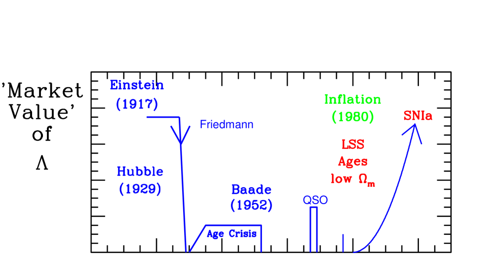
Figure 1.1: The variation in the accepted value of the cosmological constant over time, from Freedman (1999).

It was originally invoked by Einstein because of the belief at the time that the universe was static. It was only when Hubble discovered that the universe is expanding and the FLRW models were generally accepted that an alternative route was available. This led to the standard big bang cosmology.

It is possible to achieve an accelerated expansion of the universe without invoking the cosmological constant, but this requires a large negative pressure: note that gravity effectively becomes repulsive whenever the pressure is large and negative enough, that is when

$$\mu+3p<0;$$ (1.1)

(where $\mu,~{}p$ are the energy density and pressure respectively) which is precisely when the strong energy condition fails (see §5.1.1 and §6.2). This happens because $\mu+3p$ is the effective gravitational mass. This is most elegantly shown in the Raychaudhuri equation (2.37), which is the fundamental equation of gravitational attraction. It says that the expansion rate $\theta$ changes with time according to

$$\dot{\theta}\sim-{\textstyle\frac{1}{2}}(\mu+3p)+\Lambda$$ (1.2)

where $\Lambda$ is the cosmological constant. In fact, it is easy to see (§2.5.1) that a cosmological constant is indistinguishable from a constant pressure; we may acknowledge this and identify the effective active gravitational mass with

$$\mu+3p-2\Lambda$$ (1.3)

which shows why a cosmological constant may lead to an increasing expansion rate.

Central to this thesis is an assumption we shall keep: the Copernican principle. There is no precise definition of the Copernican principle. In its weakest form it states that we are not at the center of the universe. This is not particularly useful for this thesis, so we will take a slightly stronger version: we are in a ‘typical’ location as observers in the universe. (This is sometimes known as the weak cosmological principle; Ellis, 1975.) Stronger still would be to say that all observers are equivalent, which would then force homogeneity. This is the cosmological principle (CP), and cannot be satisfied for inhomogeneous models. The CP follows from (either version of) the Copernican principle if we assume perfect isotropy about ourselves. With these assumptions we are lead to the standard homogeneous and isotropic model of the universe. We aim to show that the homogeneity of the universe does not follow from the Copernican principle, given that observations about ourselves are not perfectly isotropic. This allows the CP, and thus the standard model to be questioned.

Although it essentially a philosophical assumption, the Copernican principle must be taken seriously (Ellis 1975): in order to reject an inhomogeneous cosmological model on the basis of its conflicting with the observed isotropy of the universe it is necessary to consider all observer positions and to show that for most observers in that spacetime the anisotropy observed is too large to be compatible with observations. We could adopt this view of the Copernican principle in this thesis, but, for simplicity, we will require consistency with observations for all observers – our results will thus be rather stronger than is strictly required by the Copernican Principle. In fact, it is only really possible to consider the weaker version of the Copernican principle when the spatial sections of the universe have finite volume (or, at least, when the number of observers, as measured by the integral over the spatial sections of the number density of particles – cf. §4.2 – is finite), otherwise the expression ‘most observers’ has very little meaning. For infinite universes the stronger version of the Copernican principle must be adopted. With our stronger definition we are thus prepared for all eventualities (although it will turn out that the models we consider are all ‘finite’).

Non-central locations are rarely considered in the literature in the analysis of inhomogeneous cosmologies however, owing to the mathematical difficulties that this usually entails. Having said that, Humphreys et al. (1997) made a study of Tolman-Bondi models from a non-central location and applied their results to a ‘Great Attractor’ model. Most other non-central analyses, however, look only at perturbations of standard FLRW models.

Having adopted (a strong version of) the Copernican principle, the question then arises as to whether the observed isotropy of the universe, when required to hold at every point, forces homogeneity, thus validating the CP. Well, the nearby universe is distinctly lumpy, so it would be difficult to claim there is isotropy on that basis. However, the CMB is isotropic to one part in 10⁵. Together with the EGS theorem (Ehlers, Geren and Sachs (1968)), or rather, the almost EGS theorem of Stoeger, Maartens, and Ellis (1995) this allows us to say that within our past lightcone the universe is almost FLRW (ie, almost homogeneous and isotropic), provided the fundamental observers in the universe follow geodesics (that is, as long as the fundamental fluid is dust). What the almost EGS theorem achieves is to provide support for the CP without the need to blithely assume the (near) isotropy of every observable: isotropy of the CMB alone is enough to ensure the validity of the CP (for geodesic observers).

The EGS theorem is crucial to this thesis. It states that if all observers in an expanding dust universe see an isotropic radiation field, then that universe is FLRW. As the observed high isotropy of the CMB so well established, we can combine it with the Copernican principle as the starting point of this work. We generalise the EGS theorem to the case of an irrotational perfect fluid (ie, allowing for acceleration), to find a class of models which generalise the FLRW model. These models are a subclass of the inhomogeneous Stephani spacetimes with symmetry. We are left with a class of spacetimes which allow an isotropic CMB for all observers. We then study these models from all observer locations to show that these inhomogeneous models are acceptable given present observational constraints. They thus satisfy the Copernican principle while being inhomogeneous.

A number of inhomogeneous or anisotropic cosmological models have been studied in relation to the CP. The homogeneous but anisotropic Bianchi and Kantowki-Sachs models (Kantowski and Sachs 1966; see Ellis 1998, §6 and references therein) have been investigated with regard to the time evolution of the anisotropy. It can be shown, for example, that there exist Bianchi models for which a significant phase of their evolution is spent in a near-FLRW state, even though at early and late times they may be highly anisotropic (again, see §6 of Ellis 1998 and references therein). Of the inhomogeneous models that arise in cosmological applications, by far the most common are the (Lemaître-)Tolman-Bondi dust spacetimes (Tolman 1934; Bondi 1947). These are used both as global inhomogeneous cosmologies – probably the most important papers being Hellaby and Lake (1984, 1985), studying geometrical aspects, and Rindler and Suson (1989), Goicoechea and Martin-Mirones (1987), Schneider and Célérier (1999), Célérier (1999), and Maartens et al. (1996) investigating observational aspects – and also as models of local, nonlinear perturbations (over- or under-densities) in an FLRW background (Tomita 1995, 1996; Moffat and Tatarski 1995; Krasiński 1998; Nakao et al. 1995). See also Krasiński (1998) for a review.

There has been some consideration of Stephani solutions (Stephani 1967a,b; see also Kramer et al. 1980 and Krasiński 1983, 1997). These are the most general conformally flat perfect fluid solutions – and obviously therefore contain the FLRW models. They differ from FLRW models in general because they have inhomogeneous pressure, which leads to acceleration of the fundamental observers. Da̧browski and Hendry (1998) fitted a certain subclass of these models to the first SNIa data of Perlmutter et al. (1997) using a low-order series expansion of the magnitude-redshift relation for central observers derived in Da̧browski (1995), and found that they were significantly older than the FLRW models that fit that data.

One unusual feature of the Stephani models is their matter content. The usual perfect-fluid interpretation precludes the existence of a barotropic equation of state in general (because the density is homogeneous but the pressure is not), although they can be provided with a strict thermodynamic scheme (Bona and Coll 1988) – it has recently been shown explicitly that they may be given a physically reasonable interpretation (Sussman 1999). Moreover, even individual fluid elements can behave in a rather exotic manner, having negative pressure, for example (cf. §5.1.1). For these reasons, amongst others, Lorenz-Petzold (1986) has claimed that Stephani models are not a viable description of the universe, but Krasiński (1997, p.170) argues rather vigorously that this conclusion is incorrect, as do we. Other cosmologies have sometimes been ruled out a priori because the stress-energy tensor does not behave in the correct manner, or for other reasons such as the lack of an FLRW limit – see Krasiński (1997) for a complete review. However, it has become increasingly difficult to avoid the conclusion that the expansion of the universe is accelerating, with the type Ia supernovae data being the latest and strongest evidence for this. It may be taken as evidence that there is some kind of ‘negative pressure’ driving the expansion of the universe. In standard FLRW models, this must correspond to an inflationary scenario, with $\Lambda>0$, or a matter content of the universe which is mostly scalar field (‘quintessence’ – see Frampton 1999; Liddle 1999; Coble, Dodelson and Frieman 1997; Liddle and Scherrer 1998; see also Goliath and Ellis 1998 for a discussion of the dynamical effects associated with $\Lambda$). Either way, the real universe is behaving in a manner that is at odds with ‘everyday’ physics, so it is not appropriate to rule out Stephani models for exhibiting similar behaviour.

We now briefly review FLRW models and then discuss the observational constraints primarily used in this thesis.

1.1 The FLRW Models

The standard model of modern cosmology are homogeneous and isotropic expanding FLRW models. They are parameterised by three independent functions of time; $\{H_{0},\Omega_{0},\Omega_{\Lambda}\}$. The present day expansion rate is given by the Hubble constant, $H_{0}$; the density of matter today is given by $\Omega_{0}$, which is normalised with $H_{0}$; and $\Omega_{\Lambda}$ represents a possible cosmological constant.

These models expand from a big bang into the universe’s present state. The models may recollapse after a finite time or expand indefinitely into the future: they are called ‘closed’ or ‘open’ respectively depending on this future fate, while the limiting case between the two possibilities is called ‘flat’. The different possibilities depend on whether the matter density and cosmological constant (in the combination $\Omega_{0}+\Omega_{\Lambda}$) are large enough to halt the expansion of the universe. The time since the big bang depends crucially on $H_{0}$. A significant problem facing cosmologists is an accurate measurement of these parameters.

1.2 The Hubble constant

The Hubble constant, $H_{0}$, represents the present day expansion rate of the universe. It is estimated, not surprisingly, by measuring the recession velocities of nearby galaxies, which move according to the Hubble law;

$$v\approx H_{0}d,$$ (1.4)

where $v$ is the recession velocity and $d$ is the distance to nearby galaxies. (This relation holds only in the ‘local’ universe.)

Measuring Hubble’s constant has proved to be extremely difficult in practice; despite 70 years searching it still would be difficult to claim anything better than 10% accuracy. In fact it is only within the past few years that the ‘factor of 2’ uncertainty has been resolved. One of the biggest problems lies in calculating distance accurately: this becomes more difficult the further away galaxies lie. Distant galaxies are preferable because their random or peculiar velocities are substantially smaller than the Hubble expansion. The most common method of distance measurement is to use the observed magnitude. To infer distance from this one must obviously know the actual luminosity – and one must therefore use objects which have a narrow range of intrinsic luminosity which is independent of distance. A good example of such an object are Cepheid variables which pulsate regularly – the period of which is known to correlate to their luminosity. The most promising example of distant standard candles are the supernovae Ia (SNIa), which can outshine whole galaxies – and are thus observable to great distances. The maximum brightness, and subsequent light curve shape is know to correlate to luminosity. Other examples include spiral galaxies whose rotation velocity correlates with luminosity (the Tully-Fisher relation).

The main error in using these standard candles arises because they must be combined together to obtain $H_{0}$ via the ‘cosmic distance ladder’. One of the main sources of error in $H_{0}$ lies in finding the period-luminosity relation for Cepheids, which is a consequence of errors in the distance to the Large Magellanic Cloud.

These methods are finally reaching conclusion, albeit with different groups reaching slightly different mean values; finally, however, all the results seem to be consistent. At the 95% confidence level Freedman (1999b) quotes $57<H_{0}<85$ km s^-1 Mpc^-1. Despite this many would argue that $H_{0}=65\pm 5$ km s^-1 Mpc^-1 is a safe bet; see Trimble and Aschwanden (1999) for an entertaining discussion of this.

There are promising new methods for measuring $H_{0}$ from observations of objects at large distances. These include time delay in gravitational lensing events, and use of the Sunyaev-Zel’dovich effect from the X-ray emitting gas in clusters affecting the cosmic microwave background (CMB) spectrum.

Measurements of $H_{0}$ from gravitational lensing make use of distant variable sources which are lensed, producing multiple images. The different paths the light travels will result in a time delay effect, which is measurable. Measurements of the angular separation of the two images then allow $H_{0}$ to be determined. The problem with this is that the mass distribution of the lensing galaxy will not be known independently. This, combined with the difficulty of finding a suitable system makes gravitational lensing a test for the future (Freedman 1999a).

The Sunyaev-Zel’dovich effect is the scattering of the CMB photons off electrons in the X-ray emitting gas of rich clusters (Sunyaev-Zel’dovich 1969). This results in a change in the CMB spectrum. The X-ray flux is distance dependent, but the SZ temperature fluctuations are not, therefore $H_{0}$ may be determined. As with the gravitational lensing measurements, it is still early days, with large uncertainties, and only a few clusters.

1.3 The Density Parameters $\Omega_{0}$ and $\Omega_{\Lambda}$, and the Curvature

In the standard model the energy density, curvature, and cosmological constant are all related by the normalised (with respect to $H_{0}$) parameters, $\{\Omega_{0},\Omega_{k},\Omega_{\Lambda}\}$ by

$$\Omega_{0}+\Omega_{\Lambda}+\Omega_{k}=1.$$ (1.5)

We see that determining any two of the three will give the third. Determining these will determine the origin and fate of the universe.

The density and curvature of the universe remain in question, and this uncertainty has led to the dark matter problem. The main problems here lie in the fact that the luminous matter density of galaxies nearby give a value of $\Omega_{0}\sim 0.01$ (Big Bang Nucleosynthesis also gives similar, but slightly higher, results – see Wainwright and Ellis 1997, or Olive, 1999, for details), while dynamical studies of the same galaxies suggest that $\Omega_{0}\mathrel{\vbox{\hbox{\tiny\ooalign{\raise 3.25pt\hbox{$>$}\crcr$\sim$}}}}0.3$ – ie, they are gravitationally bound by a far greater mass than we see. This means that most of the matter in the galaxies is ‘dark’. There have been plenty of suggestions as to what it may be, see Carr (1994) for further details. In addition to this the latest SNIa measurements suggest that the deceleration parameter $q_{0}={\textstyle\frac{1}{2}}\Omega_{0}-\Omega_{\Lambda}<0$ which necessarily implies that $\Omega_{\Lambda}>0$ – see figure 2.7. If the SNIa results are correct, then there is no way, in the standard model, to avoid invoking a cosmological constant or scalar field model.

Measurements of these parameters from ‘local’ ($z\sim 1$) observations (eg, SNIa) , and from observations of the CMB ($z\sim 1000$) complement each other (Tegmark, Eisenetein and Hu, 1998a; Tegmark et al., 1998b; Eisenstein, Hu and Tegmark, 1998a,b; see also Tegmark, 1999; White, 1998; Efstathiou et al., 1998; and §2.8.2). The SNIa determine the quantity $\Omega_{0}-\Omega_{\Lambda}$, while CMB results give $\Omega_{0}+\Omega_{\Lambda}$ (ie, the curvature). See §2.8.2 for details why. This means that the two data sets will give all of $\{\Omega_{0},\Omega_{k},\Omega_{\Lambda}\}$.

Supernovae Results

Riess et al. (1998), Schmidt et al. (1998) and Perlmutter et al. (1999). These all suggest that $\Lambda$ is distinctly non-zero and positive. Accurate measurements of the SNIa constrain the deceleration parameter because they measure the change in the expansion rate with distance. They are observed at roughly half the age of the universe.

The primary errors in using SNIa for the determination of the density parameters are similar as for $H_{0}$. In addition, the SNIa may evolve (as has been suggested by Drell, Loredo, and Wasserman 1999) ie, intrinsic brightness changes with distance. This simply amounts to not knowing precisely enough how intrinsically bright the objects in question are at the time of emission. The SNIa have caused such a stir initially, because they are thought not have this problem.

Perlmutter et al. (1999) quote their best fit as $\Omega_{0}=0.73,~{}\Omega_{\Lambda}=1.32$; while their best fit results assuming a flat universe is $\Omega_{0}=0.28,~{}\Omega_{\Lambda}=0.72$ with errors of $\pm 0.14$. Regardless of the type of fit its claimed that $\Lambda>0$ at the 99% confidence level. The other group achieve similar results.

CMB Measurements

The CMB was discovered in 1965 by Penzias and Wilson, and interpreted as a ‘relic’ of the big bang by Dicke et al. (1965).

The CMB is observed today to be a blackbody at a temperature of $T_{0}=2.734\pm 0.01$K, with a dipole moment of $T_{1}=3.343\pm 0.016\times 10^{-3}$K and quadrupole moment as big as $T_{2}=2.8\times 10^{-5}$K (see Mather et al., 1994; Partridge 1997 for details and references). It was emitted at a time when the radiation was no longer hot enough to keep Hydrogen ionised, causing it to decouple from matter, which happens at $T_{{}_{\mathsf{dec}}}\sim 3000$K. At this time, the small perturbations (created by inflation) which were present in the universe left their mark on the CMB surface. The baryons (electrons and protons) fell into the potential wells created by the small perturbations. Because the baryons were still coupled to the photons, the photon pressure acted as a restoring force against the motion of the baryons into the potential wells. This led to acoustic oscillations. These oscillations may be decomposed into their Fourier modes, with the first acoustic peak at $l\sim 200/\sqrt{\Omega_{0}+\Omega_{\Lambda}}$ – see figure 1.2.

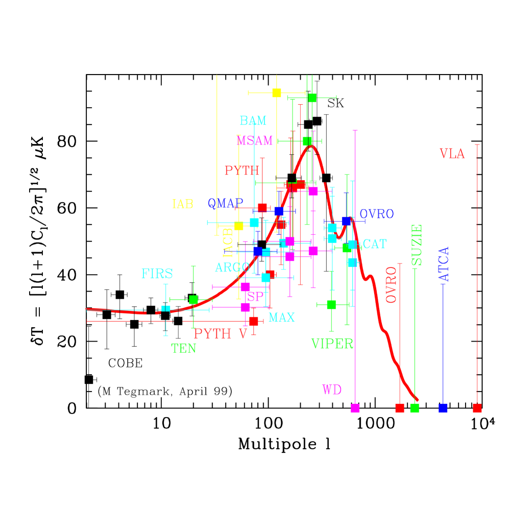
Figure 1.2: The CMB multipoles as a function of temperature.
From Max Tegmark’s home page: http://www.sns.ias.edu/~max/foregrounds.html.

Because the position of the first Doppler peak depends essentially only on the curvature, the CMB is a good test of $\Omega_{0}+\Omega_{\Lambda}$. From figure 1.2, we can see that the curve favours a flat universe – the first peak is around $l\sim 200$. The estimated curvature is $\Omega_{0}+\Omega_{\Lambda}=1\pm 0.2$. See Turner (1999), Straumann (1999), or Rocha (1999).

This is still a preliminary result, but the issue should be settled soon with some new satellites being launched in the next year or so (eg, MAP, Plank, etc.). These results are not particularly relevant for the work contained in this thesis.

The SNIa and CMB measurements may be combined to give more accurate information on the density parameters – see §2.8.2. They can also be used to find the ‘equation of state’ of the universe; see Perlmutter et al. (1999), or Efstathiou (1999).

1.4 Age

There are two ways to determine the age of the universe. Determinations of the ages of ‘old’ objects such as globular clusters in the local universe provide a lower bound to the age of the universe. Alternatively, given a model of the universe, a measurement of $H_{0}$ provides an estimate of the age of the universe. Both are plagued with uncertainty and there has been considerable disagreement until very recently, with globular clusters being significantly older than the age as implied by the expansion rate.

From $H_{0}$ we can obtain a range of ages from 8 Gyr for an Einstein-de Sitter model, all the way up to 16-17 Gyr for a low density flat model, both depending on the value of $H_{0}$. Given a set of parameters $\{H_{0},\Omega_{0},\Omega_{\Lambda}\}$ the age can be calculated simply from

$$T=\int_{0}^{T}dt=\int_{0}^{\infty}{\frac{dz}{H(z)(1+z)}},$$ (1.6)

where $H(z)$ is given by equation (2.135).

Measuring the ages of globular clusters is quite a complicated process; it is based on a number of complementary methods. It combines estimates from stellar models, with separate evaluations of the stars in the clusters turning off from the main sequence. As stellar models are not perfect uncertainties of about 7% arise. The largest uncertainties in the cluster ages arise from estimating their distance – and hence their intrinsic luminosities which are required to calibrate the stellar models. Distance estimates are made from parallax measurements, and from distance indicators such as RR Lyraes. As in estimating $H_{0}$, calibration of these stars relies on knowing the distance to the Large Magellanic Cloud, which again introduces considerable uncertainties.

The ages of the globular clusters have traditionally been quite high – certainly too high for a flat $\Lambda=0$ model, and led to the ‘age problem’ as it was known. However recent recalibration of RR-Lyraes has led to a considerable reduction in the ages of these to about 11-14 Gyrs (Chaboyer et al., 1998; Krauss, 1999); also recent parallax measurements using the Hipparcos satellite confirm these results (Reid, 1997; Gratton et al., 1997). For a high value of $H_{0}$ or a high density model, the margin of error between cosmological and globular cluster ages is still very small. See Freedman (1999b) for discussion and references.

The age of the universe is important for this thesis because the Stephani models we consider here were initially put forward for their ‘naturally’ high age, and as a solution to the age crisis (Da̧browski and Hendry, 1998). We constrain the Stephani models later using the age.

Chapter 2 Relativistic Cosmology

The goal of cosmology is to find a model that best describes the universe on any particular scale, preferably on all scales. The framework which is usually used, and will be used throughout this thesis, is that of General Relativity (GR) as discussed in eg, Wald (1984); Stephani (1990); Misner, Thorne and Wheeler (1971); Schutz (1990); Hawking and Ellis (1973); that is to say spacetime is a manifold, which has a geometry described by a Lorentz metric $g_{ab}$, and associated connection $\Gamma^{a}_{~{}bc}$, containing matter whose physical properties are described by the energy-momentum tensor, $T_{ab}$. The curvature of the spacetime is felt via the Riemann tensor, $R_{abcd}$, which gives the lack of commutivity of derivatives when parallel transporting vectors in a curved manifold (Schutz 1980);

$$\left(\nabla_{a}\nabla_{b}-\nabla_{b}\nabla_{a}\right)\xi_{c}=R_{abcd}\xi^{d},$$ (2.1)

for any vector field $\xi^{a}$; these are the Ricci identities. The curvature of spacetime and the matter content interact via Einstein’s field equations,

$$G_{ab}\!\!\mathrel{\vbox{\hbox{ \ooalign{\raise 4.75pt\hbox{${\textsf{\tiny{\,def}}}$}\crcr$=$}}}}R_{ab}-{\textstyle\frac{1}{2}}Rg_{ab}=T_{ab}-\Lambda g_{ab},$$ (2.2)

where $G_{ab}$ is the Einstein tensor, $R_{ab}$ and $R$ are the Ricci tensor and scalar, and $\Lambda$ is the cosmological constant. These equations give local conservation of energy from the geometry of the spacetime. The vector formed by taking the 4-divergence of $T_{ab}$, $\nabla_{b}T^{ab}$ represents the local creation or loss of energy. The Bianchi identities,

$$\nabla_{[a}R_{bc]}^{\phantom{h}\phantom{h}de}=0,$$ (2.3)

when twice contracted (over the $ac$ and $ed$ indices) imply $\nabla_{b}G^{ab}=0$, from (2.2) so that,

$$\nabla_{b}T^{ab}=0,$$ (2.4)

so that energy is locally conserved.

For any model of the universe, we must bear in mind that we have to extract observational predictions from it; (2.2) are not particularly intuitive. Rather than just start from a metric and see what we get, it is desirable to break (2.2) down into a simpler (or at least more intuitive) set of equations while retaining their covariant character, and at the same time introducing quantities that are directly measurable.

2.1 The Covariant 1+3 Formulation of Fluids in GR

In this thesis, we don’t make much use of the 1+3 formalism (Ehlers 1993), but it is necessary for the results of §2.3, and §3.2, and also for a proper understanding of modern relativistic cosmology.

For a complete cosmological model one must specify not only a metric defined on a manifold, but also a family of fundamental observers. These worldlines may be used to represent galaxies at late times (where the galaxies sit on the worldlines) or radiation at early times. It is usually assumed however that at any particular epoch there is, on average, one dominant or fundamental congruence of worldlines, eg, that defined by the CMB. The combinations of such a set of fluids will be described briefly later. These worldlines will have a velocity

$$u^{a}\!\!\mathrel{\vbox{\hbox{ \ooalign{\raise 4.75pt\hbox{${\textsf{\tiny{\,def}}}$}\crcr$=$}}}}\frac{dx^{a}}{d\tau},$$ (2.5)

where $\tau$ is the proper time measured along the worldlines, such that $u_{a}u^{a}=-1$; ie, it is timelike. This velocity field is very important and its properties (together with a matter description) can be used to give invariant definitions of many cosmological models.

This velocity field can be used to look at tensors along these worldlines, and orthogonal to them. This is the ‘1+3’ splitting of the spacetime into ‘temporal’ and ‘spatial’ parts; it is also covariant because $u^{a}$ can be defined uniquely and without any coordinates which would be required for splitting the spacetime into space+time.

Given $u^{a}$ we define a projection tensor by

$$h_{ab}\!\!\mathrel{\vbox{\hbox{ \ooalign{\raise 4.75pt\hbox{${\textsf{\tiny{\,def}}}$}\crcr$=$}}}}g_{ab}+u_{a}u_{b},$$ (2.6)

which defines a ‘3-metric’ orthogonal to the congruence, and satisfies

$$h_{a}^{\phantom{h}a}=3,\phantom{h}h_{ab}u^{b}=0;$$ (2.7)

ie, it is orthogonal to $u^{a}$, it therefore projects things into the instantaneous rest space of the congruence.

We also make use of the projected alternating tensor (a generalisation of the Levi-Civita symbol)

$$\eta_{abc}\!\!\mathrel{\vbox{\hbox{ \ooalign{\raise 4.75pt\hbox{${\textsf{\tiny{\,def}}}$}\crcr$=$}}}}\eta_{abcd}u^{d},$$ (2.8)

where

$$\eta_{abcd}\!\!\mathrel{\vbox{\hbox{ \ooalign{\raise 4.75pt\hbox{${\textsf{\tiny{\,def}}}$}\crcr$=$}}}}-\sqrt{|g|}\delta^{0}{}_{[a}\delta^{1}{}_{b}\delta^{2}{}_{c}\delta^{3}{}_{d]}$$ (2.9)

is the spacetime alternating tensor (the 4D Levi-Civita symbol).

We use angle brackets to denote the projected, symmetric, trace-free part of a 2nd rank tensor,

$$F_{\langle ab\rangle}\!\!\mathrel{\vbox{\hbox{ \ooalign{\raise 4.75pt\hbox{${\textsf{\tiny{\,def}}}$}\crcr$=$}}}}\left(h_{(a}^{\phantom{h}c}h_{b)}^{\phantom{h}d}-{\textstyle\frac{1}{3}}h_{ab}h^{cd}\right)F_{cd},$$ (2.10)

(and for a 1-form or vector, $K_{\langle a\rangle}\!\!\mathrel{\vbox{\hbox{ \ooalign{\raise 4.75pt\hbox{${\textsf{\tiny{\,def}}}$}\crcr$=$}}}}h_{a}^{\phantom{h}b}K_{b}$) so that any projected 2nd rank tensor has the irreducible covariant decomposition

$$F_{ab}={\textstyle\frac{1}{3}}Fh_{ab}+\eta_{abc}F^{c}+F_{\langle ab\rangle},$$ (2.11)

where $F=F_{cd}h^{cd}$ is the spatial trace, and $F_{a}={\textstyle\frac{1}{2}}\eta_{abc}F^{bc}$ is the spatial dual vector of the antisymmetric part of $F_{ab}$. In the 1+3 covariant formalism, all irreducible quantities are either scalars, projected vectors or projected, symmetric, trace-free tensors.

With this projection tensor and velocity field, we can define two derivatives; firstly, differentiation along the fluid flow – a time derivative, denoted by a dot,

$$\dot{F}_{ab}\!\!\mathrel{\vbox{\hbox{ \ooalign{\raise 4.75pt\hbox{${\textsf{\tiny{\,def}}}$}\crcr$=$}}}}u^{c}\nabla_{c}F_{ab};$$ (2.12)

and also the derivative projected orthogonal to the flow lines – a spatial derivative,

$$\widetilde{\nabla}_{c}F_{ab}\!\!\mathrel{\vbox{\hbox{ \ooalign{\raise 4.75pt\hbox{${\textsf{\tiny{\,def}}}$}\crcr$=$}}}}h^{d}_{\phantom{h}c}h^{e}_{\phantom{h}a}h^{f}_{\phantom{h}b}\nabla_{d}F_{ef}.$$ (2.13)

This new tensor is entirely orthogonal to $u^{a}$; contraction of any index with $u^{a}$ is zero. $\widetilde{\nabla}_{a}$ is no longer a proper 3-dimensional covariant derivative however, because in general,

$$\widetilde{\nabla}_{[a}\widetilde{\nabla}_{b]}Q\neq 0;$$ (2.14)

which means that the congruence is no longer orthogonal to the spacelike surfaces.

The covariant derivative of any scalar can be split into orthogonal and parallel parts;

$$\nabla_{a}Q=\widetilde{\nabla}_{a}Q-\dot{Q}u_{a};$$ (2.15)

while derivatives of vectors and tensors can be split into their irreducible covariant bits, see Maartens, Gebbie and Ellis (1999) for the equations.

2.1.1 Kinematics of the Fundamental Congruence

The derivative of the fundamental congruence $\nabla_{a}u_{b}$ can be split into irreducible quantities. These are:

• The expansion,

  $$\theta\!\!\mathrel{\vbox{\hbox{ \ooalign{\raise 4.75pt\hbox{${\textsf{\tiny{\,def}}}$}\crcr$=$}}}}\nabla_{a}u^{a}=\widetilde{\nabla}_{a}u^{a},$$ (2.16)

  which is the trace of the derivative of $u^{a}$ and also the 3-divergence of the congruence. It represents the volume rate of expansion of the fluid elements. In general, one can associate a fundamental or average length scale by

  $$\frac{1}{3}\theta\equiv\frac{\dot{\ell}}{\ell}$$ (2.17)

  which describes the volume change of the fluid.

• The acceleration,

  $$\dot{u}^{a}\!\!\mathrel{\vbox{\hbox{ \ooalign{\raise 4.75pt\hbox{${\textsf{\tiny{\,def}}}$}\crcr$=$}}}}u^{b}\nabla_{b}u^{a},$$ (2.18)

  is the time rate of change of $u^{a}$; it describes motion of the flow moving under forces other than gravity alone. This comment can be understood by thinking about a Schwarzschild black hole: if someone sits at a constant proper distance from the black hole, then the force of gravity will pull them into the center. In order to stay at a constant proper distance from it, then there must be some non-gravitational force pushing outwards. Acceleration is zero if and only if the flow is geodesic (freely falling observers).

• The shear,

  $$\sigma_{ab}\!\!\mathrel{\vbox{\hbox{ \ooalign{\raise 4.75pt\hbox{${\textsf{\tiny{\,def}}}$}\crcr$=$}}}}\widetilde{\nabla}_{\langle a}u_{b\rangle},$$ (2.19)

  is the rate of shearing of the congruence; ie, the trace-free symmetric part, which describes how the congruence will distort in time. While it doesn’t affect the volume change of the congruence, the relative distances of objects will change because of the presence of shear. Its magnitude is defined by $\sigma^{2}\!\!\mathrel{\vbox{\hbox{ \ooalign{\raise 4.75pt\hbox{${\textsf{\tiny{\,def}}}$}\crcr$=$}}}}{\textstyle\frac{1}{2}}\sigma_{ab}\sigma^{ab}$, and $\sigma=0$ $\Leftrightarrow$ $\sigma_{ab}=0$.

• The rotation,

  $$\omega_{ab}\!\!\mathrel{\vbox{\hbox{ \ooalign{\raise 4.75pt\hbox{${\textsf{\tiny{\,def}}}$}\crcr$=$}}}}\widetilde{\nabla}_{[a}u_{b]}$$ (2.20)

  describes the rate of rotation of the congruence; it is the orthogonally projected anti symmetric part of the derivative of the flow. Objects will change their position in the sky because of rotation. It also has magnitude $\omega^{2}\!\!\mathrel{\vbox{\hbox{ \ooalign{\raise 4.75pt\hbox{${\textsf{\tiny{\,def}}}$}\crcr$=$}}}}{\textstyle\frac{1}{2}}\omega_{ab}\omega^{ab}$, with $\omega=0$ $\Leftrightarrow$ $\omega_{ab}=0$. We also define a rotation vector by $\omega^{a}\!\!\mathrel{\vbox{\hbox{ \ooalign{\raise 4.75pt\hbox{${\textsf{\tiny{\,def}}}$}\crcr$=$}}}}{\textstyle\frac{1}{2}}\eta^{abc}\omega_{bc}$.

The covariant derivative can now be decomposed as

$$\nabla_{a}u_{b}=-u_{a}\dot{u}_{b}+{\textstyle\frac{1}{3}}\theta h_{ab}+\sigma_{ab}+\omega_{ab},$$ (2.21)

giving a covariant representation of the changing congruence in terms of invariantly defined quantities – which also give a physical breakdown of different aspects to the kinematics of the congruence. This equation is of fundamental importance to cosmology – and relativity in general – and was first given by Ehlers (1961), translated recently as Ehlers (1993). See also Ellis (1971).

We are now in a position to understand and expand (2.14), and a derivation is probably useful:

$$\widetilde{\nabla}_{a}\widetilde{\nabla}_{b}Q \!\!\!\!= \!\!\!\!h_{a}^{\phantom{h}d}h_{b}^{\phantom{h}e}\nabla_{d}h_{e}^{\phantom{h}c}\nabla_{c}Q$$

$$\!\!\!\!= \!\!\!\!\dot{Q}\widetilde{\nabla}_{b}u_{a}+h_{a}^{\phantom{h}c}h_{b}^{\phantom{h}d}\nabla_{c}\nabla_{d}Q,$$

which implies, using (2.20),

$$\widetilde{\nabla}_{[a}\widetilde{\nabla}_{b]}Q=-\omega_{ab}\dot{Q}$$ (2.22)

for any scalar field $Q$. This result was first presented in Bruni, Dunsby, and Ellis (1992). It shows explicitly that the fundamental congruence will define a spatial ‘3-metric’ orthogonal to the flow line if and only if the rotation is zero, because that is when $\widetilde{\nabla}$ defines a proper covariant derivative.

2.1.2 The Energy-Momentum Tensor

Regardless of the particular matter present, any energy-momentum tensor can be decomposed with respect to the chosen fundamental congruence in the following manner:

$$T_{ab}\!\!\mathrel{\vbox{\hbox{ \ooalign{\raise 4.75pt\hbox{${\textsf{\tiny{\,def}}}$}\crcr$=$}}}}\mu u_{a}u_{b}+ph_{ab}+2q_{(a}u_{b)}+\pi_{ab},$$ (2.23)

with each of the quantities having a physical interpretation:

• The relativistic energy density

  $$\mu\!\!\mathrel{\vbox{\hbox{ \ooalign{\raise 4.75pt\hbox{${\textsf{\tiny{\,def}}}$}\crcr$=$}}}}u^{a}u^{b}T_{ab}=u^{a}u^{b}G_{ab}-\Lambda;$$ (2.24)

• The isotropic pressure

  $$p\!\!\mathrel{\vbox{\hbox{ \ooalign{\raise 4.75pt\hbox{${\textsf{\tiny{\,def}}}$}\crcr$=$}}}}{\textstyle\frac{1}{3}}h^{ab}T_{ab}={\textstyle\frac{1}{3}}h^{ab}G_{ab}+\Lambda;$$ (2.25)

• The energy flux, or relativistic momentum density

  $$q_{a}\!\!\mathrel{\vbox{\hbox{ \ooalign{\raise 4.75pt\hbox{${\textsf{\tiny{\,def}}}$}\crcr$=$}}}}T_{\langle a\rangle b}u^{b},$$ (2.26)

  which can be interpreted as the heat flow relative to $u^{a}$; it satisfies $q_{a}u^{a}=0$;

• The anisotropic pressure

  $$\pi_{ab}\!\!\mathrel{\vbox{\hbox{ \ooalign{\raise 4.75pt\hbox{${\textsf{\tiny{\,def}}}$}\crcr$=$}}}}T_{\langle ab\rangle},$$ (2.27)

  which is trace-free, $\pi_{a}^{\phantom{h}a}=0$, and $u^{a}\pi_{ab}=0$.

2.1.3 The Splitting of the Weyl Tensor

The trace-free part of the Riemann tensor is the Weyl tensor, $C_{abcd}$, which describes the free gravitational field – tidal forces and gravitational waves – and to some extent describes the null structure of the spacetime. It is defined by

$$R_{abcd}=C_{abcd}+g_{a[c}R_{d]b}-{\textstyle\frac{1}{3}}Rg_{a[c}g_{d]b}.$$ (2.28)

In the 1+3 splitting of the spacetime, the Weyl tensor can be split too, into ‘electric’ and ‘magnetic’ parts:

$$E_{ab} \!\!\mathrel{\vbox{\hbox{ \ooalign{\raise 4.75pt\hbox{${\textsf{\tiny{\,def}}}$}\crcr$=$}}}}C_{abcd}u^{c}u^{d}$$ (2.31)

$$H_{ab} \!\!\mathrel{\vbox{\hbox{ \ooalign{\raise 4.75pt\hbox{${\textsf{\tiny{\,def}}}$}\crcr$=$}}}}{\textstyle\frac{1}{2}}\eta_{acde}C^{cd}_{\phantom{h}\phantom{h}bf}u^{e}u^{f}.$$ (2.34)

Both of them are symmetric, trace-free, and orthogonal to $u^{a}$.

2.2 Splitting Einstein’s Equations

If we take Einstein’s equations (2.2), the twice-contracted Bianchi identities, the Bianchi identities (2.3), or using (2.28)

$$\nabla^{d}C_{abcd}=\nabla_{[a}\left(-R_{b]c}+{\textstyle\frac{1}{6}}Rg_{b]c}\right)$$ (2.35)

and the Ricci identities (2.1) for the congruence $u^{a}$, and separate out all the independent parts, we arrive at a set of evolution and constraint equations describing the structure of spacetime. Not all of these are used in this thesis, but they are included for completeness.

Evolution:

• The energy conservation equation

  $$\dot{\mu}+\theta(\mu+p)+\widetilde{\nabla}_{a}q^{a}=-2\dot{u}_{a}q^{a}-\sigma_{ab}\pi^{ab};$$ (2.36)

  shows that, for a perfect fluid, the expansion correlates directly to the change in energy density along the flow lines;

• The Raychaudhuri equation (expansion evolution)

  $$\dot{\theta}+{\textstyle\frac{1}{3}}\theta^{2}=\widetilde{\nabla}_{a}\dot{u}^{a}+\dot{u}_{a}\dot{u}^{a}-2\sigma^{2}+2\omega^{2}-{\textstyle\frac{1}{2}}(\mu+3p)+\Lambda,$$ (2.37)

  which is the equation of gravitational attraction. This shows that a positive cosmological constant, or rotation, or acceleration will make the expansion rate increase – which is the accepted scenario at present, see later – whereas shear will slow the expansion rate. In a sense this is obvious; one would expect the ‘rotation of the universe’ to increase the expansion rate, and similarly a large negative pressure (or a positive cosmological constant – see (2.65)) will do the same;

• The momentum conservation equation

  $$\dot{q}^{\langle a\rangle}+{\textstyle\frac{4}{3}}\theta q^{a}+\widetilde{\nabla}^{a}p+\widetilde{\nabla}_{b}\pi^{ab}=-\sigma^{ab}q_{b}-(\mu+p)\dot{u}^{a}-\dot{u}_{b}\pi^{ab}-\eta^{abc}\omega_{b}q_{c},$$ (2.38)

  which shows that a perfect fluid can have acceleration only if there are spatial pressure gradients present;

• The shear and rotation evolution equations

  $$\dot{\omega}^{\langle a\rangle}+{\textstyle\frac{2}{3}}\theta\omega^{a} \!\!\!\!= \!\!\!\!{\textstyle\frac{1}{2}}\eta^{abc}\widetilde{\nabla}_{b}\dot{u}_{c}+\sigma^{ab}\omega_{b},$$ (2.39)

  $$\dot{\sigma}^{\langle ab\rangle}+{\textstyle\frac{2}{3}}\theta\sigma^{ab} \!\!\!\!= \!\!\!\!\widetilde{\nabla}^{\langle a}\dot{u}^{b\rangle}+\dot{u}^{\langle a}\dot{u}^{b\rangle}-\sigma^{\langle a}_{\phantom{h}\phantom{h}c}\sigma^{b\rangle c}-\omega^{\langle a}\omega^{b\rangle}-E^{ab}+{\textstyle\frac{1}{2}}\pi^{ab};$$ (2.40)

  the second equation shows that a fluid with $\omega_{a}=\sigma_{ab}=\dot{u}_{a}=0$ will have the electric part of the Weyl tensor proportional to the anisotropic pressure.

• The evolution of $E_{ab}$ and $H_{ab}$,

  $$\dot{E}^{\langle ab\rangle}+\theta E^{ab}-\eta^{cd\langle a}\widetilde{\nabla}_{c}H^{b\rangle}_{\phantom{h}d}+{\textstyle\frac{1}{2}}\dot{\pi}^{\langle ab\rangle}=-{\textstyle\frac{1}{2}} \!\!\!\![\widetilde{\nabla}^{\langle a}q^{b\rangle}+(\mu+p)\sigma^{ab}]+3\sigma^{\langle a}_{\phantom{h}\phantom{h}c}\left(E^{b\rangle c}-{\textstyle\frac{1}{6}}\pi^{b\rangle c}\right)$$

  $$-\dot{u}^{\langle a}q^{b\rangle}-{\textstyle\frac{1}{6}}\theta\pi^{ab} \!\!\!\!+ \!\!\!\!\eta^{cd\langle a}\left(2\dot{u}_{c}H^{b\rangle}_{\phantom{h}d}+\omega_{c}[E^{b\rangle}_{\phantom{h}d}+{\textstyle\frac{1}{2}}\pi^{b\rangle}_{\phantom{h}d}]\right),$$ (2.41)

  $$\dot{H}^{\langle ab\rangle}+\theta H^{ab}+\eta^{cd\langle a}\widetilde{\nabla}_{c}E^{b\rangle}_{\phantom{h}d}-{\textstyle\frac{1}{2}}\eta^{cd\langle a}\widetilde{\nabla}_{c}\pi^{b\rangle}_{\phantom{h}d} \!\!\!\!= \!\!\!\!3\sigma^{\langle a}_{\phantom{h}\phantom{h}c}H^{b\rangle c}+{\textstyle\frac{3}{2}}\omega^{\langle a}q^{b\rangle}$$ (2.42)

  $$\!\!\!\!- \!\!\!\!\eta^{cd\langle a}\left(2\dot{u}_{c}E^{b\rangle}_{\phantom{h}d}-\omega_{c}H^{b\rangle}_{\phantom{h}d}-{\textstyle\frac{1}{2}}\sigma^{b\rangle}_{\phantom{h}c}q_{d}\right).$$

Constraint:

• The shear and vorticity divergence equations

  $$\widetilde{\nabla}_{a}\omega^{a} \!\!\!\!= \!\!\!\!\dot{u}_{a}\omega^{a}$$ (2.43)

  $$\widetilde{\nabla}_{b}\sigma^{ab} \!\!\!\!= \!\!\!\!{\textstyle\frac{2}{3}}\widetilde{\nabla}^{a}\theta-\eta^{abc}\left(\widetilde{\nabla}_{b}\omega_{c}+2\dot{u}_{b}\omega_{c}\right)-q^{a}.$$ (2.44)

  The second equation is crucial in §3.2, where it is used to set energy flux equal to zero in a QCDM model with an isotropic radiation field.

• The ‘curl $\sigma$’ equation

  $$\eta^{cd\langle a}\widetilde{\nabla}_{c}\sigma^{b\rangle}_{\phantom{h}d}-H^{ab}=2\dot{u}^{\langle a}\omega^{b\rangle}+\widetilde{\nabla}^{\langle a}\omega^{b\rangle}$$ (2.45)

• The $E_{ab}$ and $H_{ab}$ divergence equations

  $$\widetilde{\nabla}_{b}E^{ab}-3\omega_{b}H^{ab} \!\!\!\!= \!\!\!\!{\textstyle\frac{1}{3}}[\widetilde{\nabla}^{a}\mu-\theta q^{a}]+{\textstyle\frac{1}{2}}[\sigma^{ab}q_{b}-\widetilde{\nabla}_{b}\pi^{ab}]$$ (2.46)

  $$\!\!\!\!~{}~{}~{}~{}~{}~{}~{}+\eta^{abc}\left(\sigma_{bd}H^{d}_{\phantom{h}c}-{\textstyle\frac{3}{2}}\omega_{b}q_{c}\right),$$

  $$\widetilde{\nabla}_{b}H^{ab}+3\omega_{b}E^{ab} \!\!\!\!= \!\!\!\!{\textstyle\frac{1}{2}}\omega_{b}\pi^{ab}-(\mu+p)\omega^{a}$$ (2.47)

  $$~{}~{}~{}~{}~{}-\eta^{abc}\left({\textstyle\frac{1}{2}}\widetilde{\nabla}_{b}q_{c}+\sigma_{bd}[E^{d}_{\phantom{h}c}+{\textstyle\frac{1}{2}}\pi^{d}_{\phantom{h}c}]\right).$$

2.3 1+3 Splitting Under a Conformal Transformation

A conformal transformation is an angle preserving transformation that changes lengths and volumes. The importance of these types of transformations lies in the fact that, under a conformal transformation, the null structure of the spacetime is preserved: indeed, it trivially follows that the causal structure is preserved. We also have the important property that the the Weyl tensor, $C_{abc}^{\phantom{abc}d}$, is invariant (note that one index must be raised) so that a conformal transformation will introduce no tidal forces or gravitational waves; that is, a conformal transformation will only introduce ‘non-gravitational’ forces and matter into the new spacetime (by changing $R_{ab}$ and thus the matter tensor $T_{ab}$ via Einstein’s equations).

We perform the conformal transformation

$$g_{ab}=e^{2Q}\hat{g}_{ab},\phantom{h}u^{a}=e^{-Q}\hat{u}^{a},\phantom{h}u_{a}=e^{Q}\hat{u}_{a};$$ (2.48)

where $Q>0$ is an arbitrary function, $u^{a}$ is a velocity vector with respect to $g_{ab}$: $g_{ab}u^{a}u^{b}=u_{a}u^{a}=-1$; and $\hat{u}^{a}$ is the conformally related (parallel) velocity vector, and is normalised with respect to $\hat{g}_{ab}$: $\hat{g}_{ab}\hat{u}^{a}\hat{u}^{b}=-1$. The covariant derivative of any one-form field $v_{a}$ transforms as

$$\nabla_{a}v_{b}=\widehat{\nabla}_{a}v_{b}-2Q_{(a}v_{b)}+g_{ab}Q^{c}v_{c},$$ (2.49)

where $Q_{a}\equiv Q_{,a}=\widetilde{\nabla}_{a}Q-\dot{Q}u_{a}$. The expansion ($\theta=\nabla_{a}u^{a}$), acceleration ($\dot{u}^{a}=u^{b}\nabla_{b}u^{a}$), rotation ($\omega_{ab}=\widetilde{\nabla}_{[a}u_{b]}$), and shear ($\sigma_{ab}=\widetilde{\nabla}_{\langle a}u_{b\rangle}$) of the two velocity congruences are related by:

$$\hat{\theta} \!\!\!\!= \!\!\!\!e^{Q}(\theta-3\dot{Q})$$

$$\hat{\dot{u}}_{a} \!\!\!\!= \!\!\!\!\dot{u}_{a}-\widetilde{\nabla}_{a}Q$$

$$\hat{\omega}_{ab} \!\!\!\!= \!\!\!\!e^{-Q}\omega_{ab}$$

$$\hat{\sigma}_{ab} \!\!\!\!= \!\!\!\!e^{-Q}\sigma_{ab}.$$ (2.50)

The equation for the acceleration corrects equation (6.14) of Kramer et al. (1980). These show that a conformal transformation mat induce acceleration and expansion into the new spacetime, by not shear or rotation: in particular, a conformally flat model must have shear and rotation vanishing (as in eg, the Stephani models considered later). With respect to $g_{ab}$, a dot denotes differentiation along the fluid flow – a time derivative, $\dot{F}_{ab}=u^{c}\nabla_{c}F_{ab}$; and $\widetilde{\nabla}_{a}$ is the derivative projected orthogonal to the flow lines – a spatial derivative, $\widetilde{\nabla}_{c}F_{ab}=h^{d}_{\phantom{h}c}h^{e}_{\phantom{h}a}h^{f}_{\phantom{h}b}\nabla_{d}F_{ef}$, where $h_{ab}=g_{ab}+u_{a}u_{b}$ is the usual projection tensor.

The Einstein tensor transforms as (see Wald 1982)

$$G_{ab}=\hat{G}_{ab}-2\nabla_{a}Q_{b}-2Q_{a}Q_{b}+g_{ab}\left[2\nabla_{c}Q^{c}-Q^{2}\right],$$ (2.51)

where $\hat{G}_{ab}$ is the Einstein tensor of $\hat{g}_{ab}$, and $Q^{2}=Q_{a}Q^{a}$. For clarity with the above, we decompose derivatives of $Q$ into time and space derivatives:

$$Q_{a}=\widetilde{\nabla}_{a}Q-\dot{Q}u_{a},$$

$$\nabla_{b}Q_{a}= \!\!\!\widetilde{\nabla}_{a}\widetilde{\nabla}_{b}Q+u_{a}u_{b}\left(\ddot{Q}-\dot{u}^{c}\widetilde{\nabla}_{c}Q\right)-\dot{Q}\left(\frac{1}{3}\theta h_{ab}+\sigma_{ab}-\omega_{ab}\right)$$ (2.52)

$$\!\!+2u_{(a}\left[-\widetilde{\nabla}_{b)}\dot{Q}+\frac{1}{3}\theta\widetilde{\nabla}_{b)}Q+\left(\sigma_{b)}^{\phantom{h}c}+\omega_{b)}^{\phantom{h}c}\right)\widetilde{\nabla}_{c}Q\right].$$

We also write $\hat{T}_{ab}=\hat{G}_{ab}$, and $T_{ab}=G_{ab}$ as general fluids, both with respect to $u^{a}$:

$$\hat{G}_{ab}=\hat{\mu}\hat{u}_{a}\hat{u}_{b}+\hat{p}\hat{h}_{ab}+2\hat{q}_{(a}\hat{u}_{b)}+\hat{\pi}_{ab},$$ (2.53)

$${G}_{ab}=\mu u_{a}u_{b}+ph_{ab}+2{q}_{(a}u_{b)}+{\pi}_{ab};$$ (2.54)

where $\{\hat{\mu},\hat{p},\hat{q}_{a},\hat{\pi}_{ab}\}$, and $\{\mu,p,q_{a},\pi_{ab}\}$ are the energy density, isotropic pressure, heat flux, and anisotropic pressure of $\hat{G}_{ab}$ and $G_{ab}$ respectively.

We can decompose $G_{ab}$ given by (2.51) into the fluid variables in (2.54) by using (2.52) in the following covariant manner:

$$\mu \!\!\!\!= \!\!\!\!u^{a}u^{b}G_{ab}=e^{2Q}\hat{\mu}-3\dot{Q}\left(\dot{Q}-\frac{2}{3}\theta\right)-2\widetilde{\nabla}_{a}\widetilde{\nabla}^{a}Q+\widetilde{\nabla}_{a}Q\widetilde{\nabla}^{a}Q,$$ (2.55)

$$p \!\!\!\!= \!\!\!\!\frac{1}{3}h^{ab}G_{ab}=e^{2Q}\hat{p}+\left(\dot{Q}-\frac{4}{3}\theta\right)\dot{Q}-2\ddot{Q}+\frac{4}{3}\widetilde{\nabla}_{a}\widetilde{\nabla}^{a}Q-\frac{5}{3}\widetilde{\nabla}_{a}Q\widetilde{\nabla}^{a}Q$$

$$~{}~{}~{}~{}~{}~{}~{}~{}~{}~{}~{}~{}~{}~{}~{}~{}~{}~{}~{}~{}~{}~{}~{}~{}~{}~{}~{}~{}~{}~{}~{}~{}~{}~{}~{}~{}~{}~{}~{}~{}~{}~{}~{}~{}~{}~{}~{}~{}~{}~{}~{}~{}~{}~{}~{}~{}~{}+2\dot{u}_{c}\widetilde{\nabla}^{c}Q,$$

$$q_{a} \!\!\!\!= \!\!\!\!-u^{b}G_{\langle a\rangle b}=e^{Q}\hat{q}_{a}-2\widetilde{\nabla}_{a}\dot{Q}+2\left(\frac{1}{3}\theta-\dot{Q}\right)\widetilde{\nabla}_{a}Q+2\left(\sigma_{a}^{\phantom{h}b}+\omega_{a}^{\phantom{h}b}\right)\widetilde{\nabla}_{b}Q$$ (2.57)

$$\pi_{ab} \!\!\!\!= \!\!\!\!G_{\langle ab\rangle}=\hat{\pi}_{ab}+2\dot{Q}\sigma_{ab}-2\widetilde{\nabla}_{\langle a}\widetilde{\nabla}_{b\rangle}Q-2\widetilde{\nabla}_{\langle a}Q\widetilde{\nabla}_{b\rangle}Q.$$ (2.58)

2.4 Relativistic Thermodynamics

Any realistic cosmological model must include some sort of thermodynamic scheme. This means that we expect the laws of thermodynamics to hold throughout the evolution of the universe.

Together with the conservation equations (2.4) the energy-momentum tensor (2.23), which lead to the equations (2.36) and (2.38), there are a number of other conservation equations which one may or may not impose upon the fluid. See Ehlers (1971) for derivations and a discussion of kinetic theory in GR.

Firstly, we normally assume that the comoving number density is conserved; ie,

$$\nabla_{a}(N^{a})\equiv 0,$$ (2.59)

where $N^{a}\!\!\mathrel{\vbox{\hbox{ \ooalign{\raise 4.75pt\hbox{${\textsf{\tiny{\,def}}}$}\crcr$=$}}}}nu^{a}$ and $n$ is the number density of particles – see Krasinski (1997), or Maartens (1996). Now, (2.59) is equivalent to the condition

$$\dot{n}+\theta n=0\phantom{h}\Leftrightarrow\phantom{h}n\ell^{3}={\mathrm{const.}},$$ (2.60)

where (2.17) was used to demonstrate that the number of particles in a comoving volume is constant.

However, in a more realistic model this may not be true at some stages of the evolution, see for example Gunzig et al. (1997) where a particle creation rate is introduced to model creation of radiation due to inflation. Other generalisations include adding a viscous pressure term; eg, Coley, van den Hoogen, and Maartens (1996), or Maartens (1995).

The First Law of Thermodynamics

The first law is the Gibbs equation which applies in equilibrium:

$$TdS\equiv d\left(\frac{\mu}{n}\right)+pd\left(\frac{1}{n}\right),$$ (2.61)

where $S$ is the entropy density, and $T$ is the temperature of the fluid; or

$$T\nabla_{a}Sdx^{a}=\nabla_{a}\left[\frac{\mu}{n}\right]dx^{a}+p\nabla_{a}\left[\frac{1}{n}\right]dx^{a};$$ (2.62)

which becomes, upon dividing by an increment of proper time along the congruence, and substituting from (2.60),

$$\dot{S}=\frac{1}{Tn}\left(\dot{\mu}+\theta(\mu+p)\right)$$ (2.63)

which shows that $\dot{S}=0$ for a perfect fluid (cf, (2.36)): ie, entropy per particle along a particular flow line remains constant.

The Second Law

Entropy flux is generally defined as a vector;

$$S^{a}=Snu^{a}+\frac{R^{a}}{T}$$ (2.64)

where $R^{a}$ represents all dissipative processes, and $S$ and $T$ are related by ((2.61) – ie, they are scalars defined in local equilibrium). In the simplest cases $R^{a}$ is assumed zero, or equated with the energy flux. The second law states $\nabla_{a}S^{a}\geq 0$, where equality applies in equilibrium (where $R^{a}=0$).

Equations (2.59), and (2.61) comprise a thermodynamic scheme which implies that the right hand side of (2.61) has an integrating factor – see Krasiński, Quevedo and Sussman (1997). These are additional constraints on cosmological models. (This is used in §3.1.3.)

2.5 Fluids in Cosmology

Equation (2.23) is a general equation describing any fluid. Different types of fluid have different energy-momentum tensors, which we will now discuss in order of importance for cosmological models.

The most important fluids used in cosmology are dust solutions, often with a cosmological constant. The simplest of these are the FLRW models, which are generally believed to represent the universe on a suitably large scale; perturbations of these models give a more realistic representation of the universe. However, simple does not mean correct and therefore other models have been studied to give a different view of the universe; among these are the dust Lemaitre-Tolman (LT) models and Bianchi models – the latter often used because they are ‘close to FLRW’ for some suitable length of time, and therefore give a better understanding of FLRW models themselves.

Generalisation of a simple dust solution to a perfect fluid is a necessary, but not always simple, task if one wants a model of the universe before recombination; most solutions of Einstein’s equations which are used as cosmological models are perfect fliuds (in particular, a scalar field can always be written as a perfect fluid).

Here it will be useful to note that a cosmological constant can always be absorbed into the energy-momentum tensor by redefining the density and pressure.

$$G_{ab} \!\!\!\!= \!\!\!\!T_{ab}+\Lambda g_{ab}$$ (2.65)

$$\!\!\!\!= \!\!\!\!\mu u_{a}u_{b}+\Lambda h_{ab}-\Lambda u_{a}u_{b}$$

$$\!\!\!\!= \!\!\!\!(\mu-\Lambda)u_{a}u_{b}+\Lambda h_{ab};$$

ie, a perfect fluid with constant pressure. A cosmological constant does not need to be studied separately in the other perfect fluid cases.

2.5.1 Perfect Fluids and Dust Models

A perfect fluid occurs when $\pi_{ab}=q^{a}=0$; in the case of dust (‘CDM’) we also have $p=0$, which necessarily implies (by (2.38)) that the fundamental congruence is geodesic; $\dot{u}^{a}\equiv 0$. These models are implicitly in equilibrium; that is, the dynamics are completely reversible and no heat is generated from friction or anything else ($\dot{S}=0$).

From the energy conservation equation (2.36), we get the simple relation for the expansion,

$$\theta=-\frac{\dot{\mu}}{(\mu+p)};$$ (2.66)

and similarly for the acceleration (2.38),

$$\dot{u}_{a}=-\frac{\widetilde{\nabla}_{a}p}{\mu+p}.$$ (2.67)

However, the Raychaudhuri equation remains unchanged – emphasising that it is an equation relating the important kinematic quantities of the flow, rather than the more complex anisotropic pressures, energy flux or Weyl curvature. We can substitute (2.66) and (2.67) into the Raychaudhuri equation (2.37) to get a second order differential equation for the matter quantities.

From the Gibbs relation (2.61) (which defines the temperature) the entropy of a perfect fluid cannot change along the congruence (cf, 2.63);

$$\dot{S}=0.$$ (2.68)

The adiabatic speed of sound is given by

$$c_{s}=\sqrt{\frac{\dot{p}}{\dot{\mu}}}$$ (2.69)

which must be less than the speed of light.

Perfect fluids can be split into different types, according to their dependence of $\mu$ on $p$.

A Barotropic Equation of State

Generally a useful simplifying assumption to make upon the fluid is that of a barotropic equation of state (EOS). It is a fairly ad hoc assumption which simply requires that the pressure depends only on the density: $p\equiv p(\mu)$. It is adopted usually for mathematical simplicity rather than for any physical reasons. This functional dependence can in principle take any form. There are a few results which follow from this simple EOS.

From (2.67) we get

$$\widetilde{\nabla}_{[a}\dot{u}_{b]}=0\phantom{h}\Leftrightarrow\phantom{h}\eta^{abc}\widetilde{\nabla}_{b}\dot{u}_{c}=0,$$ (2.70)

so that rotation is conserved,

$$\dot{\omega}^{\langle a\rangle}+{\textstyle\frac{2}{3}}\theta\omega^{a}=\sigma^{ab}\omega_{b},$$ (2.71)

cf (2.39).

For these types of cosmological models the entropy is a global constant; (from 2.61),

$$\widetilde{\nabla}_{a}S=0;$$ (2.72)

which implies $\nabla_{a}S=0$. This is an isentropic fluid – an unrealistic situation.

Dust: $p\equiv 0$.

This is the most common fluid form used for a cosmological model. Its simplicity lies in making the motion geodesic, and thus eliminating many terms in Einstein’s equations.

In this case the energy density scales inversely with volume. In general, one defines the characteristic length scale of a model by

$$\frac{1}{3}\theta=\frac{\dot{\ell}}{\ell},$$ (2.73)

hence, by (2.66) we have

$$\frac{3\dot{\ell}}{\ell}=-\frac{\dot{\mu}}{\mu}\Rightarrow\mu\sim{\ell}^{-3}.$$ (2.74)

Dust is a particularly simple cosmological model to deal with. It models the late universe of galaxies as ‘particles’ of dust moving under gravity alone. It requires that the random velocities of the galaxies be negligible – ie, the temperature is very low, so may not be used in the radiation dominated era.

$\gamma$-law equation of state

This is a classic simple type of perfect fluid, which can describe a number of situations. We have an equation of state of the form

$$p=(\gamma-1)\mu:\phantom{h}1\leq\gamma\leq 2,$$ (2.75)

where $\gamma$ is constant. $\gamma=1$ corresponds to dust, described above. Again, from (2.66), we have $\mu\sim{\ell}^{-3\gamma}$. The other important case is that of radiation, $\gamma=4/3$.

If $\gamma=2$, then we have a ‘stiff fluid’, in which the speed of sound equals that of light. This is, in a sense, the equation of state of the ‘ether’. It is usually discounted as a physically reasonable form of matter as it fails the energy conditions, but some scalar field models have an effective equation of state of this form. A cosmological constant may be accounted for by $\gamma=0,\mu=\Lambda$.

In the standard model (FLRW), we have a multi-fluid description: we have a mixture of (non-interacting) matter and radiation, with the radiation dominating at early times. If we have the characteristic length scale $\ell$ in an expanding universe, then radiation density falls off as $\ell^{-4}$, but the matter density of the dust decreases as $\ell^{-3}$: hence, if we proceed forward in time from the initial singularity ($\ell=0$), then radiation will dominate early on, but matter will take on the dominant role later.

2.5.2 Scalar Fields

Scalar fields are fashionable at the moment for their use in describing inflationary scenarios in the early universe, but they may be present today (quintessence). There is no need to go into any physical detail here, but the basics are required for §3.2. A scalar field has an energy-momentum tensor of the form

$$T_{ab}\!\!\mathrel{\vbox{\hbox{ \ooalign{\raise 4.75pt\hbox{${\textsf{\tiny{\,def}}}$}\crcr$=$}}}}\nabla_{a}\phi\nabla_{b}\phi-g_{ab}\left({\textstyle\frac{1}{2}}\nabla_{c}\phi\nabla^{c}\phi+V(\phi)\right),$$ (2.76)

where $V$ must satisfy the Klein-Gordon equation;

$$V^{\prime}(\phi)=\nabla^{a}\nabla_{a}\phi.$$ (2.77)

If $\nabla_{a}\phi$ is timelike then we may define the velocity field

$$u^{a}={\frac{\nabla^{a}\phi}{\sqrt{-\nabla_{b}\phi\nabla^{b}\phi}}}$$ (2.78)

so that $T_{ab}$ has the form of a perfect fluid with effective energy density and pressure

$$\mu=-{\textstyle\frac{1}{2}}\nabla_{a}\phi\nabla^{a}\phi+V(\phi),~{}~{}~{}p=-{\textstyle\frac{1}{2}}\nabla_{a}\phi\nabla^{a}\phi-V(\phi).$$ (2.79)

2.5.3 Velocity Fields

In general there is no canonical definition of the ‘correct’ fundamental velocity field to use and the energy-momentum tensor will have a different interpretation depending on the chosen congruence. That is, it is not obvious whether fundamental observers should be identified with the natural congruence in, say, a perfect fluid, or with some other velocity field (Coley and Tupper, 1983, 1984, 1985). This is fundamental to the 1+3 formalism: the decomposition above is velocity field dependent.

If we take a perfect fluid

$$T_{ab}=\hat{\mu}\hat{u}_{a}\hat{u}_{b}+\hat{p}\hat{h}_{ab}$$ (2.80)

and consider this with respect to another congruence $u^{a}$ defined such that

$$\hat{u}^{a}\!\!\mathrel{\vbox{\hbox{ \ooalign{\raise 4.75pt\hbox{${\textsf{\tiny{\,def}}}$}\crcr$=$}}}}\Gamma(u^{a}+v^{a})$$ (2.81)

with $v^{a}u_{a}=0$ (ie, $v^{i}$ is the 3-velocity relative to $\hat{u}^{a}$) and $\Gamma=1/\sqrt{1-v^{2}}$ – basically a Lorentz boost – then $T_{ab}$ will have the general form (2.23), with the relative energy densities etc., related by

$$\mu \!\!\!\!= \!\!\!\!\hat{\mu}+\Gamma^{2}v^{2}(\hat{\mu}+\hat{p})$$

$$p \!\!\!\!= \!\!\!\!\hat{p}+{\textstyle\frac{1}{3}}\Gamma^{2}v^{2}(\hat{\mu}+\hat{p})$$

$$q_{a} \!\!\!\!= \!\!\!\!\Gamma^{2}(\hat{\mu}+\hat{p})v_{a}$$

$$\pi_{ab} \!\!\!\!= \!\!\!\!\Gamma^{2}(\hat{\mu}+\hat{p})\left\{v_{a}v_{b}-{\textstyle\frac{1}{3}}v^{2}h_{ab}\right\}.$$ (2.82)

(See Wainwright and Ellis, 1997.) We can see that for a perfect fluid a relative energy flux will always be introduced by a change of velocity field. This is required for §3.2.

In the case of a general fluid with respect to another velocity field, the transformations are given in Maartens, Gebbie and Ellis (1999).

2.5.4 More General Fluids

The perfect fluids considered up to now are clearly unphysical: the entropy is constant and there is no frictional heating. While this is not a problem if all we want is a rough and ready model to work with (eg, the standard model), we require something a little more involved for a decent model of the universe: thermodynamic processes in the real universe are (probably) not reversible. Unfortunately, there doesn’t seem to be a well formulated theory of relativistic dissipative fluid mechanics, and there only seem to be a couple of cases occasionally used, such as bulk viscosity to describe inflation using the truncated Israel-Stewart theory of irreversible thermodynamics (Israel and Stewart, 1979, 1980); see Maartens (1996) for a review. See also Gariel and Le Denmat (1994).

2.6 The CMB Anisotropies

In §1.3 we discussed the observed characteristics of the anisotropies in the CMB radiation. Relativistic cosmology must explain the effects which cause these anisotropies before decoupling (ie, perturbations of the spacetime structure, density fluctuations etc.) and effects that occur after the last scattering surface which affect the size of the anisotropies as the photons travel to us (eg, lensing by structure, the Rees-Sciama effect – the changing redshift of the CMB photons as they pass through varying gravitational potentials; Rees and Sciama 1968 – interstellar dust – Finkbeiner and Schlegel 1999)

The first attempt at a relativistic treatment was by Sachs and Wolfe (1967) by integrating the null geodesics in a perturbation of a flat $\Lambda=0$ FLRW model to examine the redshift function along the null rays. This has been done in a gauge-invariant and covariant 1+3 way by Challinor and Lasenby (1998, 1999) for scalar perturbations. These approaches have been generalised by Maartens, Gebbie and Ellis (1999) to include some more non-linear effects – see also Maartens (1999), Challinor (1999), Gebbie and Ellis (1999). The essential steps, after choosing a suitable velocity field, are to decompose the photon distribution function, the collision term in the Boltzmann equation and the temperature fluctuation into spherical harmonics to get the multipole moments for an inhomogeneous spacetime.

The covariant and gauge invariant results are presented in the above references, and are a bit of a mess. In this thesis we will only require a small part of the calculations which give additional evolution equations for radiation other than those given by (2.36)-(2.42).

For a radiation field, the energy-momentum tensor is given by

$$T_{\!{}_{R}}^{ab}(x^{i})=\mu_{\!{}_{R}}u^{a}u^{b}+{\textstyle\frac{1}{3}}\mu_{\!{}_{R}}h^{ab}+2q_{\!{}_{R}}^{(a}u^{b)}+\pi_{\!{}_{R}}^{ab}=\int p^{a}p^{b}f(x^{i},p^{c})d^{3}p,$$ (2.83)

where

$$p^{a}\!\!\mathrel{\vbox{\hbox{ \ooalign{\raise 4.75pt\hbox{${\textsf{\tiny{\,def}}}$}\crcr$=$}}}}E(u^{a}+e^{a}):~{}~{}~{}E=-p^{a}u_{a},$$ (2.84)

is the photon momentum, with $e^{a}$ a unit spacelike vector, and $d^{3}p=EdEd\Omega$ is the volume element on the future null cone at $x^{i}$. $f(x^{i},p^{c})$ is the photon distribution function, which gives the number density of photons at $x^{i}$ with momenta $p^{a}$, and must satisfy the Boltzmann equation,

$${\frac{df}{dv}}={\cal C}(f),$$ (2.85)

with ${\cal C}$ being change of $f$ along the geodesics (parameterised by $v$) from all types of collisions, absorptions, etc., and which is effectively zero after decoupling. The terms in (2.83) define the first three multipole moments: $\mu_{\!{}_{R}}$ is the monopole, and represents the average temperature over the whole sky via the Stefan-Boltzmann law;

$$\left\langle T^{4}\right\rangle_{{}_{{}_{\mathsf{all~{}sky}}}}\propto\mu_{\!{}_{R}},$$ (2.86)

so if the distribution function is a Planck distribution, then the temperature is that of a black body. Any fluctuations in brightness across the sky are given by the higher order multipoles, $q_{\!{}_{R}}^{a},~{}\pi_{\!{}_{R}}^{ab},~{}\Pi^{a_{1}a_{2}\cdots a_{\ell}}$. Now, if the observers’ frame ($v^{a}$) is moving non-relativistically relative to the CMB frame ($u^{a}$) then these evolve according to

$$\dot{\mu}_{\!{}_{R}}+{\textstyle\frac{4}{3}}\theta\mu_{\!{}_{R}}+\widetilde{\nabla}_{a}q_{\!{}_{R}}^{a}+2\dot{u}_{a}q_{\!{}_{R}}^{a}+\sigma_{ab}\pi_{\!{}_{R}}^{ab} \!\!\!\!= \!\!\!\!n_{{}_{E}}\sigma_{{}_{T}}\left({\textstyle\frac{4}{3}}\mu_{\!{}_{R}}v^{2}-q_{\!{}_{R}}^{a}v_{a}\,\right)+{\cal O}[3]$$ (2.87)

$$\dot{q}_{\!{}_{R}}^{\langle a\rangle}+{\textstyle\frac{4}{3}}\theta q_{\!{}_{R}}^{a}+{\textstyle\frac{4}{3}}\mu_{\!{}_{R}}\dot{u}^{a}+{\textstyle\frac{1}{3}}\widetilde{\nabla}^{a}\mu_{\!{}_{R}} \!\!\!\!+ \!\!\!\!\widetilde{\nabla}_{b}\pi_{\!{}_{R}}^{ab}+\sigma^{a}{}_{b}q_{\!{}_{R}}^{b}+$$

$$\eta^{abc}\omega_{b}q_{\!{}_{R}c}+\dot{u}_{b}\pi_{\!{}_{R}}^{ab} \!\!\!\!= \!\!\!\!n_{{}_{E}}\sigma_{{}_{T}}\left({\textstyle\frac{4}{3}}\mu_{\!{}_{R}}v^{a}-q_{\!{}_{R}}^{a}+\pi_{\!{}_{R}}^{ab}v_{b}\right)+{\cal{O}}[3]$$ (2.88)

which are the new forms of (2.36), and (2.38) for the case when the radiation field is not quite aligned with the (baryonic) observer. There are evolution equations for all the higher order multipoles as well, which are not given in a simple fluid description: the quadrupole evolves according to

$$\dot{\pi}_{\!{}_{R}}^{\langle ab\rangle} \!\!\!\!+ \!\!\!\!{\textstyle\frac{4}{3}}\theta\pi_{\!{}_{R}}^{ab}+{\textstyle\frac{8}{15}}\mu_{\!{}_{R}}\sigma^{ab}+{\textstyle\frac{2}{5}}\widetilde{\nabla}^{\langle a}q_{\!{}_{R}}^{b\rangle}+{8\pi\over 35}\widetilde{\nabla}_{c}\Pi^{abc}$$ (2.89)

$$+ \!\!\!\!2\dot{u}^{\langle a}q_{\!{}_{R}}^{b\rangle}+2\omega^{c}\eta_{cd}{}^{\langle a}\pi_{\!{}_{R}}^{b\rangle d}+{\textstyle\frac{2}{7}}\sigma_{c}{}^{\langle a}\pi_{\!{}_{R}}^{b\rangle c}-{32\pi\over 315}\sigma_{cd}\Pi^{abcd}$$

$${}=-n_{\!{}_{E}}\sigma_{\!{}_{T}}\left({\textstyle\frac{9}{10}}\pi_{\!{}_{R}}^{ab}-{\textstyle\frac{1}{5}}q_{\!{}_{R}}^{\langle a}v^{b\rangle}-{8\pi\over 35}\Pi^{abc}v_{c}-{\textstyle\frac{2}{5}}\mu_{\!{}_{R}}v^{\langle a}v^{b\rangle}\right)+{\cal O}[3]$$

while the higher multipoles ($\ell>3$) evolve according to

$$\dot{\Pi}^{\langle A_{\ell}\rangle} \!\!\!\!+ \!\!\!\!{\textstyle\frac{4}{3}}\theta\Pi^{A_{\ell}}+\widetilde{\nabla}^{\langle a_{\ell}}\Pi^{A_{\ell-1}\rangle}+{(\ell+1)\over(2\ell+3)}\widetilde{\nabla}_{b}\Pi^{bA_{\ell}}$$ (2.90)

$${}-\ {(\ell+1)(\ell-2)\over(2\ell+3)}\dot{u}_{b}\Pi^{bA_{\ell}}+(\ell+3)\dot{u}^{\langle a_{\ell}}\Pi^{A_{\ell-1}\rangle}+\ell\omega^{b}\eta_{bc}{}^{\langle a_{\ell}}\Pi^{A_{\ell-1}\rangle c}$$

$${}-\ {(\ell-1)(\ell+1)(\ell+2)\over(2\ell+3)(2\ell+5)}\sigma_{bc}\Pi^{bcA_{\ell}}+{5\ell\over(2\ell+3)}\sigma_{b}{}^{\langle a_{\ell}}\Pi^{A_{\ell-1}\rangle b}-(\ell+2)\sigma^{\langle a_{\ell}a_{\ell-1}}\Pi^{A_{\ell-2}\rangle}$$

$${}=-n_{\!{}_{E}}\sigma_{\!{}_{T}}\left[\ \Pi^{A_{\ell}}-\Pi^{\langle A_{\ell-1}}v^{a_{\ell}\rangle}-\left({\ell+1\over 2\ell+3}\right)\Pi^{A_{\ell}a}v_{a}\ \right]+{\cal O}[3].$$

For $\ell=3$, the $\Pi^{\langle A_{\ell-1}}v^{{a_{\ell}}\rangle}$ term on the right-hand side of equation (2.90) must be multiplied by ${3\over 2}$. $n_{\!{}_{E}}$ is the free electron number density and $\sigma_{\!{}_{T}}$ is the Thompson scattering cross section. The series expansion terminates at ${\cal O}[3]={\cal O}(\epsilon v^{2},v^{3})$ where $\epsilon$ is a small parameter to represent how close the radiation and baryonic frames are: there is no neglect of physical and geometric quantities. All that is assumed is that the matter moves non-relativisticaly.

These results are required for the EGS theorem later: without them (especially without (2.89)) Theorem 1 cannot be proved in the 1+3 formalism.

2.7 Observations in the 1+3 Formalism

Observations in cosmology are made by observing light which has travelled on our past light cone. They are made essentially from one spacetime point – ‘here and now’. All we can hope to know directly from this is where the light is coming from and how it travelled here. The point of cosmology is to infer as much information about the universe as possible, hopefully with as few assumptions as possible. As a generic problem, the absolute limit to the amount we can know has been shown by Ellis et al. (1985) to be that part of the universe enclosed in our past lightcone, even assuming infinite precision in the observations (and assuming Einstein’s equations (2.2)).

The part relativistic cosmology has to play is to determine the cosmological model (or indeed the entire class of models) which fits the observations best: that is, what is the metric $g_{ab}$ and matter content $T_{ab}\equiv G_{ab}$ (and necessarily the fundamental congruence, $u^{a}$) of the universe? This is distinct from other areas of cosmology insofar as it need not, in the first approximation, describe the details of structure, or how the structure formed. It must, however, be able to describe gross features like the CMB; for example, the anisotropy of the CMB has been used to limit some global properties of $u^{a}$ such as the shear – see Ellis, Treciokas and Matravers (1983a,b); Stoeger, Maartens and Ellis (1995); Maartens, Ellis and Stoeger (1995); and Theorem 1.

We must be able to relate the light that is observed to the metric $g_{ab}$ and velocity field $u^{a}$. The most important methods are also the most direct: light observed from discrete sources, and light from the CMB.

2.7.1 Observable Quantities From Discrete Sources

The foundations of this subject come from the now ‘famous in the right circles’ paper by Kristian and Sachs (1966), who first treated the subject in a covariant manner (see also MacCallum and Ellis (1970)). Their method was to identify the various distance measures available in cosmology and relate them to redshift using the intrinsic and observed brightnesses (or equivalently, magnitudes) of the sources.

Luminosity-Distance Relations

If we observe a star to have some flux $\cal F$ that has some intrinsic luminosity $\cal L$ then its luminosity distance is defined to be

$$r_{L}\!\!\mathrel{\vbox{\hbox{ \ooalign{\raise 4.75pt\hbox{${\textsf{\tiny{\,def}}}$}\crcr$=$}}}}\sqrt{\frac{\cal L}{4\pi\cal F}}.$$ (2.91)

This is a simple extension of the variation of the brightness of objects in non-relativistic physics because the flux that we observe not only decreases because of the decreased number-density of photons, but also because each photon is losing energy due to the expansion of the universe. This loss of energy of each photon is given by its redshift, $z$;

$$1+z\!\!\mathrel{\vbox{\hbox{ \ooalign{\raise 4.75pt\hbox{${\textsf{\tiny{\,def}}}$}\crcr$=$}}}}\frac{\lambda_{{\mathrm{observed}}}}{\lambda_{{\mathrm{emitted}}}}\equiv\frac{\nu_{{\mathrm{emitted}}}}{\nu_{{\mathrm{observed}}}}=\frac{\delta t_{o}}{\delta t_{e}},$$ (2.92)

which shows redshift to be a time dilation effect. Although this last equality is true for photons, it is actually true for any null-connected points in any (smooth) spacetime. Redshift, therefore, reflects the stretching effect of expansion of spacetime; since it is a directly measurable quantity, it is of fundamental importance. It is therefore of some importance to write down other quantities in terms of redshift. There is, however, a problem, and one which is quite difficult in practice. If a galaxy is observed to have a redshift $z$ then determining how much of this is cosmological, $z_{c}$, and how much is due to the relative motions of source ($z_{e}$) and observer ($z_{o}$) requires a careful study of the galaxy movement and a knowledge of our relative motion. The redshifts are related by

$$1+z=(1+z_{c})(1+z_{o})(1+z_{e}),$$ (2.93)

although the $z_{o}$ term can be inferred from a knowledge of the CMB dipole – the CMB frame.

Redshift

Redshift can be treated in a more rigorous way. By solving Maxwell’s equations on a pseudo-Riemannian manifold in a charge and current free region, and assuming that the wavelength of light is small compared to the spacetime curvature (the geometrical optics approximation), we find that light is tangent to null surfaces of constant phase $\phi$, and therefore travels on null geodesics. So if a photon’s velocity is given by a null (geodesic) vector $k^{a}\!\!\mathrel{\vbox{\hbox{ \ooalign{\raise 4.75pt\hbox{${\textsf{\tiny{\,def}}}$}\crcr$=$}}}}\nabla^{a}\phi$ ($\Leftrightarrow$ $\nabla_{[a}k_{b]}=0$):

$$0=\nabla_{a}\phi\nabla^{a}\phi=k^{a}k_{a};\phantom{aaaa}k^{a}\nabla_{a}k^{b}=0,$$ (2.94)

(the first of these is the eikonal equation – see Ehlers and Newman 1999) then the angle between this vector and some velocity field $u^{a}$ is the relative (angular) frequency of the photon as measured by an observer traveling on $u^{a}$,

$$\omega=-u^{a}k_{a}.$$ (2.95)

This frequency is clearly observer dependent; an observer moving in a different manner would measure a different frequency (doppler shift). If a photon travels between two points then the redshift is the relative change of frequency between the two points;

$$1+z\!\!\mathrel{\vbox{\hbox{ \ooalign{\raise 4.75pt\hbox{${\textsf{\tiny{\,def}}}$}\crcr$=$}}}}\frac{\left.u_{a}k^{a}\right|_{\mathrm{e}}}{\left.u_{b}k^{b}\right|_{\mathrm{o}}}.$$ (2.96)

We can see this more explicitly by calculating the rate of change of frequency along the photon path;

$$k^{a}\nabla_{a}\omega=k^{a}\nabla_{a}(-u_{b}k^{b})=-k^{a}k^{b}\nabla_{a}u_{b}=\left(-{\textstyle\frac{1}{3}}\theta h_{ab}+\dot{u}_{a}u_{b}-\sigma_{ab}\right)k^{a}k^{b}.$$ (2.97)

$k^{a}$ is a null vector, and so can be written as a linear combination of a component parallel and orthogonal to $u^{a}$, viz;

$$k^{a}=-u_{b}k^{b}(u^{a}+e^{a}).$$ (2.98)

where $e^{a}$ is a normalised spacelike vector orthogonal to $u^{a}$: $e^{a}e_{a}=1$; $u_{a}e^{a}=0$; it simply defines the direction of the photon relative to $u^{a}$. Substituting this into (2.97) we find

$$k^{a}\nabla_{a}\omega=-\omega^{2}\left({\textstyle\frac{1}{3}}\theta+e^{a}\dot{u}_{a}+e^{a}e^{b}\sigma_{ab}\right).$$ (2.99)

It is now clear that the relative direction of the photon is important when considering frequency change; important effects also come from the kinematics of $u^{a}$. For example expansion will decrease the photon frequency and thus increase the wavelength, making it redshifted. However, the change in frequency caused by shear and acceleration is direction dependent: acceleration can either increase or decrease the frequency, depending on the direction of the incoming photon relative to the direction of acceleration; similarly shear will decrease the frequency by varying amounts depending on the direction of the incoming photon and the principle directions of the shear (ie, its eigenvectors).

The Redshift Structure of Conformally Related Spacetimes.

If we have two conformally related metrics $g_{ab}=e^{2Q}\hat{g}_{ab}$: $Q>0$, then null geodesics, $g_{ab}k^{a}k^{b}=0$, are conformally invariant:

$$k^{b}\nabla_{b}k^{a}=0\Rightarrow k^{b}\widehat{\nabla}_{b}k^{a}\propto k^{a},$$ (2.100)

where $\nabla_{a}$ and $\widehat{\nabla}_{a}$ are the covariant derivatives associated with $g_{ab}$ and $\hat{g}_{ab}$ respectively. Although the null geodesics associated with $\widehat{\nabla}_{a}$ are non-affinely parameterised, the structure of the lightcones is identical for both spacetimes (see, for example Wald 1984). The affine parameters $\lambda$, $\hat{\lambda}$ associated with the $\nabla_{a}$-geodesics and $\widehat{\nabla}_{a}$-geodesics are related by

$$\frac{d\lambda}{d\hat{\lambda}}=qe^{2Q}.$$ (2.101)

with $q$ constant. Now we associate a different null vector with each metric: $k^{a}$ is tangent vector to a geodesic with affine parameter $\lambda$, and $\hat{k}^{a}$ is tangent to a geodesic with affine parameter $\hat{\lambda}$. In some basis, $x^{\alpha}$

$$\frac{d\phantom{h}}{d\hat{\lambda}}=\hat{k}^{\alpha}\frac{\partial\phantom{h}}{\partial x^{\alpha}}=qe^{2Q}\frac{d\phantom{h}}{d\lambda}=qe^{2Q}k^{\alpha}\frac{\partial\phantom{h}}{\partial x^{\alpha}};$$ (2.102)

since the basis vectors are linearly independent, we now have established the general result

$$\hat{k}^{a}=qe^{2Q}k^{a}.$$ (2.103)

Hence, if the geodesics with respect to $\widehat{\nabla}_{a}$ are known explicitly then we can find them easily for $\nabla_{a}$.

Suppose we have a metric $g_{ab}$ in comoving coordinates, $u^{\alpha}=-|g_{00}|^{-1/2}\delta^{\alpha}_{0}$, which is conformally related to another metric $\hat{g}_{ab}$ and there exists a coordinate transformation $x^{\alpha^{\prime}}(x^{\alpha})$ : $g_{\alpha\beta}\longrightarrow g_{\alpha^{\prime}\beta^{\prime}}$ where $g_{\alpha^{\prime}\beta^{\prime}}=\exp{[2Q(x^{\gamma^{\prime}})]}\hat{g}_{\alpha^{\prime}\beta^{\prime}}$ explicitly in the primed coordinate system. This means that the frequency of a photon travelling along a null geodesic becomes

$$u_{\alpha}k^{\alpha}=u_{\alpha}\frac{\partial x^{\alpha}}{\partial x^{\alpha^{\prime}}}k^{\alpha^{\prime}}=-|g_{00}|^{-1/2}\delta^{\alpha}_{0}\frac{\partial t}{\partial x^{\alpha^{\prime}}}k^{\alpha^{\prime}}=-\frac{|g_{00}|^{-1/2}\delta^{\alpha}_{0}}{qe^{2Q}}\frac{\partial t}{\partial x^{\alpha^{\prime}}}\hat{k}^{\alpha^{\prime}}$$ (2.104)

It is then straight forward to show that if $g_{\alpha^{\prime}\beta^{\prime}}$ is in comoving coordinates the redshift becomes

$$1+z=\frac{\left.u_{a}k^{a}\right|_{{}_{\mathsf{G}alaxy}}}{\left.u_{b}k^{b}\right|_{{}_{\mathsf{O}bserver}}}=\frac{\left.u_{0}k^{0}\right|_{{}_{G}}}{\left.u_{0}k^{0}\right|_{{}_{O}}}=e^{{Q|_{{}_{O}}}-{Q|_{{}_{G}}}}(1+\hat{z}).$$ (2.105)

where $\hat{z}$ is the redshift associated with $\hat{g}_{ab}$.

Area and Luminosity Distance

In addition to (2.91) as a distance measure, we can also measure the angular size of an object, $d\Omega$. If this object has an intrinsic proper area $dS$, then the area distance is defined by the ratio of these;

$$r_{A}^{2}\!\!\mathrel{\vbox{\hbox{ \ooalign{\raise 4.75pt\hbox{${\textsf{\tiny{\,def}}}$}\crcr$=$}}}}\frac{dS}{d\Omega}.$$ (2.106)

This is related to the luminosity distance (2.91) by the reciprocity theorem, which states

$$r_{L}=r_{A}(1+z)^{2},$$ (2.107)

as first proved by Etherington (1933). It is essentially a geometrical result, but can also be viewed as a time dilation effect, relating geodesics traveling up and down the null cone. See figure 2.1.

Figure 2.1: An observer measuring the area distance of a galaxy.

Area distance is measurable, and can be found by integrating the geodesic deviation equation – see MacCallum and Ellis (1970). Using (2.107), and (2.91) we can relate the metric to directly measurable quantities: redshift, luminosity and area distance;

$${\cal{F}}=\frac{{\cal{L}}}{4\pi r_{A}^{2}(1+z)^{4}}.$$ (2.108)

The Magnitude-Redshift Relation

If we take the logarithm of (2.108) we get the magnitude-redshift relation;

$$m-M-25=5\log_{10}r_{L}.$$ (2.109)

As it stands though, (2.109) is virtually useless until a cosmological model is given (or, at the very least, a metric). However, the cunning Kristian and Sachs (1966) managed to expand $r_{A}$ in a power series in $z$, and thus making a generalised magnitude-redshift relation. The result of that expansion is, in the notation of MacCallum and Ellis (1970),

$$m \!\!\!\!- \!\!\!\!M-25=5\log_{10}z-5\log_{10}\left.K^{a}K^{b}\nabla_{a}u_{b}\right|_{o}+{\textstyle\frac{5}{2}}\log_{10}e\left\{\left[\left.4-\frac{K^{a}K^{b}K^{c}\nabla_{a}\nabla_{b}u_{c}}{(K^{d}K^{e}\nabla_{d}u_{e})^{2}}\right|_{O}\right]z\right.$$ (2.110)

$$\!\!\!\!- \!\!\!\!\left[2+\left.\left.\frac{R_{ab}K^{a}K^{b}}{6(K^{c}K^{d}\nabla_{c}u_{d})^{2}}-\frac{3(K^{a}K^{b}K^{c}\nabla_{a}\nabla_{b}u_{c})^{2}}{4(K^{d}K^{e}\nabla_{d}u_{e})^{4}}+\frac{K^{a}K^{b}K^{c}K^{d}\nabla_{a}\nabla_{b}\nabla_{c}u_{d}}{3(K^{e}K^{f}\nabla_{e}u_{f})^{3}}\right]\!\!\right|_{O}z^{2}\right\}$$

$$\!\!\!\!~{}~{}~{}~{}~{}~{}~{}~{}~{}~{}~{}~{}~{}~{}~{}~{}~{}~{}~{}~{}~{}~{}~{}~{}~{}~{}~{}~{}~{}~{}~{}~{}~{}~{}~{}~{}~{}~{}~{}~{}~{}~{}~{}~{}~{}~{}~{}~{}~{}~{}~{}~{}~{}~{}~{}~{}~{}~{}~{}~{}~{}~{}~{}~{}~{}~{}~{}~{}~{}~{}~{}+{\cal O}(z^{3}),$$

where

$$K^{a}\!\!\mathrel{\vbox{\hbox{ \ooalign{\raise 4.75pt\hbox{${\textsf{\tiny{\,def}}}$}\crcr$=$}}}}\frac{k^{a}}{\left.u^{b}k_{b}\right|_{O}}\phantom{xxxx}\hbox{ie,}\phantom{xxxx}\left.K^{a}\right|_{O}=\left.-(u^{a}+e^{a})\right|_{O}.$$ (2.111)

Obviously, (2.110) is extremely complicated for a general cosmological model – even for the lowest order terms. It is also questionable how accurate this series expansion will be when truncated at low order in redshift. Certainly it will be useless for $z>1$ unless the exact function $m(z)$ has a very special form, or all terms $>{\cal O}(z)$ die off very rapidly – see figures 2.5 and 2.6.

Number Count-Distance Relations

A potentially interesting area of observational cosmology comes from number counts as a function of either redshift or magnitude. It works by simply counting galaxies at a certain redshift in a solid angle of the sky $d\Omega$ up to some limiting magnitude. If we know the (mean) density of galaxies in the spacetime then by counting how many we see in this volume will give us information about the spacetime geometry.

We do not use number-counts in this thesis (although the relevant formulae may be derived) because there is large uncertainty in the source evolution function (Mustapha, Hellaby and Ellis, 1998 – although it is unclear if their result holds if multi-colour observations are taken into account).

2.8 FLRW Models

The standard model of modern cosmology is based on a hypothesis: the Cosmological Principle (CP; Ellis 1975). One of the key issues in this thesis is the validity of the CP. The cosmological principle assumes perfect isotropy about our location and extrapolates this to every other location using the Copernican principle which necessarily implies homogeneity of the universe. Once the CP is in place then one must conclude that the universe has an FLRW form. The proof of this is intuitive, and can be found eg, in Wald (1984).

The metric of FLRW models has the form (in isotropic coordinates)

$$ds^{2}=-dt^{2}+\frac{a(t)^{2}}{(1+{\textstyle\frac{1}{4}}kr^{2})^{2}}\left(dr^{2}+r^{2}d\Omega^{2}\right)$$ (2.112)

where

$$d\Omega^{2}\!\!\mathrel{\vbox{\hbox{ \ooalign{\raise 4.75pt\hbox{${\textsf{\tiny{\,def}}}$}\crcr$=$}}}}d\vartheta^{2}+\sin^{2}\vartheta d\varphi^{2};$$ (2.113)

$k$ is a constant which characterises the spatial hypersurfaces of the model: $k<,=,>,0$ corresponds to hyperbolic, flat, or spherical geometry. Almost all the properties of the FLRW models follow from (2.112). The fundamental velocity field is given by

$$u^{0}=1;\phantom{xxx}u^{i}=0,$$ (2.114)

which has expansion

$$\theta(t)=3\frac{\dot{a}(t)}{a(t)},$$ (2.115)

with the shear, rotation, and acceleration vanishing. The energy-momentum tensor automatically has the form of a perfect fluid spacetime with respect to this congruence. In fact, the FLRW models can be invariantly classed as perfect fluid spacetimes with a fundamental congruence that has $\sigma_{ab}=\omega_{ab}=\dot{u}^{a}=0$, as can be proven from the field equations (2.36-2.47) – see Krasiński (1997).

The energy density and pressure are given by

$$\mu \!\!\!\!= \!\!\!\!3\frac{k}{a^{2}}+3\left(\frac{\dot{a}}{a}\right)^{2}-\Lambda,$$ (2.116)

$$p \!\!\!\!= \!\!\!\!-2\frac{\ddot{a}}{a}-\frac{k}{a^{2}}-\left(\frac{\dot{a}}{a}\right)^{2}+\Lambda,$$ (2.117)

as can be found using (2.24) and (2.25). Eq. (2.116) is the Friedmann equation. Combining these gives the Raychaudhuri equation (cf, (2.37))

$$\frac{\ddot{a}}{a}=-{\textstyle\frac{1}{6}}(\mu+3p)+{\textstyle\frac{1}{3}}\Lambda.$$ (2.118)

The Friedmann equation (2.116) and (2.118) gives equation (2.36).

The function $a(t)$ is free, but will have a specific form once the thermodynamics is settled upon; this usually takes the form of a barotropic equation of state, or multiple (non-)interacting fluids. As far as the standard model is concerned, the matter is assumed to be radiation until decoupling and dust thereafter. Once the matter specified (2.116) and (2.118) give a differential equation for $a(t)$, which can be solved in principle – see eg, Ellis (1998).

We can define various scalars to get an idea about the dynamics of any particular model. We define the Hubble scalar as the expansion rate

$$H\!\!\mathrel{\vbox{\hbox{ \ooalign{\raise 4.75pt\hbox{${\textsf{\tiny{\,def}}}$}\crcr$=$}}}}{\textstyle\frac{1}{3}}\theta=\frac{\dot{\ell}}{\ell}=\frac{\dot{a}}{a};$$ (2.119)

the deceleration parameter

$$q\!\!\mathrel{\vbox{\hbox{ \ooalign{\raise 4.75pt\hbox{${\textsf{\tiny{\,def}}}$}\crcr$=$}}}}-\frac{\ddot{\ell}\ell}{\dot{\ell}^{2}}=-\frac{\ddot{a}a}{\dot{a}^{2}};$$ (2.120)

and the density parameter

$$\Omega\!\!\mathrel{\vbox{\hbox{ \ooalign{\raise 4.75pt\hbox{${\textsf{\tiny{\,def}}}$}\crcr$=$}}}}\frac{\mu}{3H^{2}}=\frac{k}{H^{2}a^{2}}-\frac{\Lambda}{3H^{2}}+1.$$ (2.121)

where the last equality (from (2.116)) shows that the density parameter may be used to characterise the spatial surfaces in a $\Lambda=0$ model. We can also define

$$\Omega_{\Lambda}\!\!\mathrel{\vbox{\hbox{ \ooalign{\raise 4.75pt\hbox{${\textsf{\tiny{\,def}}}$}\crcr$=$}}}}\frac{\Lambda}{3H^{2}}$$ (2.122)

and

$$\Omega_{k}\!\!\mathrel{\vbox{\hbox{ \ooalign{\raise 4.75pt\hbox{${\textsf{\tiny{\,def}}}$}\crcr$=$}}}}-\frac{k}{a^{2}H^{2}},$$ (2.123)

which implies that the deceleration parameter becomes, using (2.118),

$$q={\textstyle\frac{1}{2}}\Omega\left(1+\frac{p}{\mu}\right)-\Omega_{\Lambda};$$ (2.124)

for dust, we have the simpler, more familiar, form

$$q={\textstyle\frac{1}{2}}\Omega-\Omega_{\Lambda}.$$ (2.125)

From (2.121) we have the normalisation condition

$$\Omega+\Omega_{\Lambda}+\Omega_{k}=1,$$ (2.126)

which means, even though all the parameters are functions of time above, that we can always characterise the curvature of the spatial surfaces in the following way:

$\Omega+\Omega_{\Lambda}>1$	closed spatial surfaces	$k>0$	$\Omega_{k}<0$
$\Omega+\Omega_{\Lambda}=1$	flat spatial surfaces	$k=0$	$\Omega_{k}=0$
$\Omega+\Omega_{\Lambda}<1$	open spatial surfaces	$k<0$	$\Omega_{k}>0$

2.8.1 The Magnitude-Redshift Relation

The magnitude-redshift relation is quite easy to derive due to the symmetry of the solution, as can be found in, eg, Peebles (1993). The key steps are outlined below. (Factors of $c$, the speed of light, are included in this section.) We are aiming to find the function $m(z)$ – a relationship between measurable quantities. The information we have about the spacetime is the metric (2.112), the Friedmann equation (2.116), and the Raychaudhuri equation (2.118). What we don’t know is the function $a(t)$ which is going to be needed if we want to compare the models to data. The usual route is to assume that the universe is dust after decoupling, and solve (2.117) for $a(t)$.

The magnitude-redshift relation in the case of $\Lambda=0$ was first solved by Mattig (1958). The general formula for vanishing pressure was first found by Kaufman (1971) after the initial generalization by Kaufman and Schucking (1971) to include $\Lambda>0$ in a closed model.

We will derive it explicitly here to facilitate comparison with later derivations for the Stephani models.

Redshift:

For a general spherically symmetric spacetime it is necessary to solve the geodesic equation for the null ray connecting the galaxy to the observer in order to determine the galaxy’s redshift. More specifically, for a null ray from the galaxy, $G$, at $(r,\tau)$ to the observer, $O$, at $(0,\tau_{0})$, the tangent vector along the ray $k^{a}$ is obtained as a solution of the geodesic equation. Once we have $k^{a}$ along the ray, though, the redshift is obtained immediately from (cf, Ellis 1998)

$$1+z={\nu_{G}\over\nu_{O}}\equiv{u_{a}k^{a}|_{G}\over u_{a}k^{a}|_{O}},$$ (2.127)

where $u^{a}$ is the four-velocity of the perfect fluid, ie, of the galaxy (G) or the observer (O). Since $u^{a}$ is a four-velocity it is normalised by

$$g_{ab}u^{a}u^{b}=-1,$$ (2.128)

and in comoving coordinates only $u^{0}$ is nonzero, so that (2.128) completely fixes $u^{a}$. However, the high symmetry of FLRW models means that the redshift can be obtained directly without having to integrate the geodesic equation – see eg, Wald (1984) for a derivation. However we can use a novel approach outlined in §2.7.1, which can be implemented if we write the metric in the conformally static form

$$ds^{2}=a(t(\eta))^{2}\left[d\eta^{2}+(1+{\textstyle\frac{1}{4}}kr^{2})^{-2}(dr^{2}+r^{2}d\Omega)\right]$$ (2.129)

where $\eta$ is the conformal time coordinate;

$$\eta\!\!\mathrel{\vbox{\hbox{ \ooalign{\raise 4.75pt\hbox{${\textsf{\tiny{\,def}}}$}\crcr$=$}}}}\int\frac{dt}{a(t)}.$$ (2.130)

Using (2.105), we immediately have (because the part in square brackets in (2.129) is static and there are no gravitational redshifts)

$$1+z={a_{0}\over a(t)};$$ (2.131)

where $a_{0}\equiv a(T)$ is the scale factor today.

Lookback time:

Consider radial null ray (ie, $d\vartheta=d\varphi=ds^{2}=0$) from a source at $(r,\tau)$ reaching the observer ($r=0$) at time $\tau_{0}$. The relationship between $\tau_{0}$, $\tau$ and $r$ can be obtained directly from the metric symmetry guaranteeing that the raypath is purely radial so it is parameterised by a function $\tau(r)$ by integrating

$${dr\over(1+{\textstyle\frac{1}{4}}kr^{2})}=c{dt\over a(t)}.$$ (2.132)

between $r$ and $r=0$. Now we have, on using (2.131),

$$\frac{dt}{a(t)}=\frac{da}{a^{2}}\frac{1}{H}=-\frac{dz}{a_{0}H},$$ (2.133)

where $H$ is given by (2.119). From (2.74) we have

$$\mu=\mu_{0}\frac{a(t)^{3}}{a_{0}^{3}}$$ (2.134)

so that (2.116) becomes, using (2.131) once again,

$$H(z)^{2}=H_{0}^{2}\left[\Omega_{0}(1+z)^{3}+\Omega_{k_{0}}(1+z)^{2}+\Omega_{{\Lambda}_{0}}\right];$$ (2.135)

where a subscript ‘$0$’ means the present day value; viz;

$$\Omega_{0}=\frac{\mu_{0}}{3H_{0}^{2}},\phantom{h}\Omega_{k_{0}}=\frac{k}{3H_{0}^{2}},\phantom{h}\Omega_{\Lambda_{0}}=\frac{\Lambda}{3H_{0}^{2}}.$$ (2.136)

Together with (2.132) this gives the function $r(z)$:

$$\left.\begin{array}[]{c|c}k>0&\frac{2}{\sqrt{k}}\tan^{-1}\left({\textstyle\frac{1}{2}}\sqrt{k}r\right)\\ k=0&r\\ k<0&\frac{2}{\sqrt{|k|}}\tanh^{-1}\left({\textstyle\frac{1}{2}}\sqrt{|k|}r\right)\end{array}\right\}={\frac{1}{a_{0}H_{0}}}\int_{0}^{z}{\frac{dz^{\prime}}{\sqrt{\Omega_{0}(1+z)^{3}+\Omega_{k_{0}}(1+z)^{2}+\Omega_{{\Lambda}_{0}}}}}.$$ (2.137)

We now have the coordinate distance as a function of redshift. We must now relate this to some measurable distance quantity.

Angular diameter distance:

Angular size distance, $r_{A}$, is the ratio of an objects physical diameter to its apparent angular diameter. As is well known, in spherically symmetric spacetimes the angular size distance of an object as seen from the centre is given by (the square root of) the coefficient in front of the angular components of the metric ($d\Omega^{2}$) evaluated at the time the light was emitted.

For any inward radial null rays, in the plane $\theta=\pi/2$, say, the angle coordinate $\phi$ obviously does not change along the path. This means that the apparent diameter, $\delta_{G}$, of a galaxy is just determined by the difference between the $\phi$ coordinates at either edge of the galaxy, at the time the light we observe was emitted (ie, at $t(r)$): $\delta_{G}=\delta\phi$. The physical diameter, $D$ of the galaxy is given from the metric (with $dt=dr=d\vartheta=0$):

$$D=\frac{a(t(r))r}{1+{\textstyle\frac{1}{4}}kr^{2}}\delta\phi={\frac{a(t(r))r}{1+{\textstyle\frac{1}{4}}kr^{2}}}\delta_{G}$$

($a(t(r))r/({1+{\textstyle\frac{1}{4}}kr^{2}})$ just being the coefficient in the angular part of the metric). The angular diameter distance, $r_{A}$, is simply defined to satisfy $D=r_{A}\delta_{G}$, so that

$$r_{A}(z)={\frac{a(t)r}{1+{\textstyle\frac{1}{4}}kr^{2}}}={\frac{a_{0}}{1+{\textstyle\frac{1}{4}}kr(z)^{2}}}{r(z)\over 1+z}$$ (2.138)

for FLRW models, where we have used (2.132) in the second equality.

The area distance can behave in quite an odd way: in non-relativistic situations when things move further away they get smaller. This is not necessarily what happens in a cosmological model: as something moves away it may get smaller at first but then start to get bigger again. This is shown in Fig 2.2 where we can see that in a closed model this refocusing occurs at some redshift.

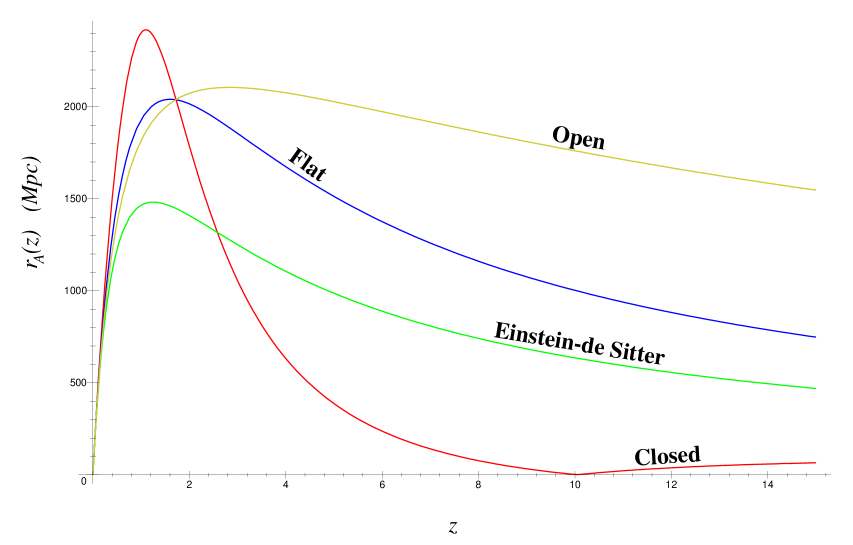
Figure 2.2: Area distance as a function of redshift for a variety of ‘standard’ models. The closed model has $\{\Omega_{0},\Omega_{\Lambda_{0}}\}$=$\{0.3,1.5\}$, Einstein-de Sitter (1932) has $\{1,0\}$, flat: $\{0.3,0.7\}$ and the open model has $\{0.1,0\}$. All the models have $H_{0}=60$ km s^-1 Mpc^-1. Note that all the curves match up for low enough redshift.

This is because the light rays are effectively traversing an expanding sphere, so a galaxy situated at the antipode to a particular observer will be spread all over the observers sky. In (dust) FLRW models, this refocusing only occurs once as $z\rightarrow\infty$ because the expansion is always just fast enough that the light rays never ‘catch it up.’

Luminosity distance:

The key to deriving the luminosity distance, $r_{L}$, is the reciprocity theorem (see Ellis and MacCallum, 1970, and references therein), which allows us to write

$$r_{L}=(1+z)^{2}r_{A}.$$ (2.139)

This equation is exact, and completely general, applying in any spacetime. Combining this with (2.138) gives

$$r_{L}(z)={\frac{(1+z)a_{0}r(z)}{1+{\textstyle\frac{1}{4}}kr(z)^{2}}}$$ (2.140)

for FLRW models. Note that we can write this in the more familiar form

$$r_{L}(z)=(1+z)a_{0}\tilde{r}(z):\left\{\begin{array}[]{c|c}\phantom{h}\tilde{r}(z)={\frac{1}{\sqrt{k}}}\sin 2\tan^{-1}{\textstyle\frac{1}{2}}\sqrt{k}r(z)&k>0,\\ \tilde{r}(z)=r(z)&k=0,\\ \phantom{h}\tilde{r}(z)={\frac{1}{\sqrt{|k|}}}\sinh 2\tanh^{-1}{\textstyle\frac{1}{2}}\sqrt{|k|}r(z)&k<0.\end{array}\right.$$ (2.141)

The function $\tilde{r}(z)$ is plotted in Fig. 2.3. Hence we have the result

$$r_{L}(z)=(1+z)a_{0}\left\{\left.\begin{array}[]{c}\sin[\sqrt{k}\\ 1\\ \sinh[\sqrt{|k|}\end{array}\right\}{\frac{1}{a_{0}H_{0}}}\int_{0}^{z}{\frac{dz^{\prime}}{\sqrt{\Omega_{0}(1+z)^{3}+\Omega_{k_{0}}(1+z)^{2}+\Omega_{{\Lambda}_{0}}}}}\right]\begin{array}[]{|c}k>0\\ k=0\\ k<0.\end{array}$$ (2.142)

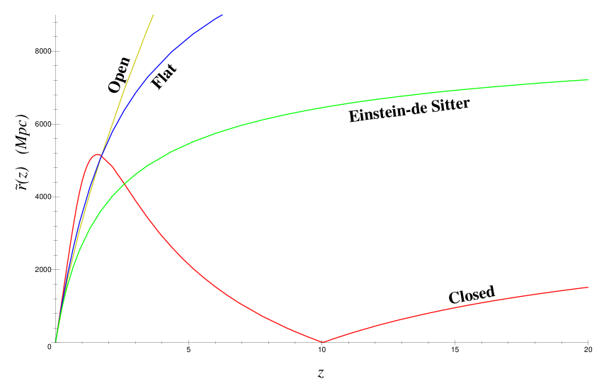
Figure 2.3: Coordinate distance as a function of redshift the models of figure 2.2.

Magnitude-redshift relation:

The magnitude-redshift relation for an object of absolute magnitude $M$ then follows from (2.142) and

$$m(z)-M \!\!\!\!- \!\!\!\!25=5\log_{10}\left.(1+z)a_{0}\times\left.\right.\right.$$ (2.150)

$$\left\{\left.\begin{array}[]{c}\sin[\sqrt{k}\\ 1\\ \sinh[\sqrt{|k|}\end{array}\right\}{\frac{1}{a_{0}H_{0}}}\int_{0}^{z}{\frac{dz^{\prime}}{\sqrt{\Omega_{0}(1+z)^{3}+\Omega_{k_{0}}(1+z)^{2}+\Omega_{{\Lambda}_{0}}}}}\right]\begin{array}[]{c}k>0\\ k=0\\ k<0.\end{array}$$

In Fig 2.4 is shown the $m-z$ relation for the same models as Fig. 2.2.

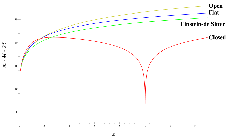
Figure 2.4: Apparent magnitude as a function of redshift for the models of figure 2.2

The closed model has the refocusing issue as before; the apparent magnitude becomes singular at that point.

As the integral in (2.150) is elliptic, it cannot be evaluated explicitly. However, a series relation can be found relatively easily;

$$m \!\!\!\!- \!\!\!\!M-25=5\log_{10}{\frac{z}{H_{0}}}$$ (2.151)

$$\!\!\!\!+ \!\!\!\!{\frac{5}{2}}\log_{10}e\left\{(1-q_{0})z+\left[{\frac{1}{4}}(3q_{0}+1)(q_{0}-1)-2\Omega_{\Lambda_{0}}\right]z^{2}+{\cal O}(z^{3})\right\}.$$

We can now consider quantitatively the comments made in §2.7.1 on the validity of the low order expansion. Consider Fig 2.5: the plot shows the difference between the exact $m(z)$ function and the series form (2.151) with an increasing power of redshift $z$ up to order $9$.

Figure 2.5: The exact magnitude-redshift relation minus the same function as a power series relation to various orders. $|m_{{}_{\mathrm{e}xact}}-m_{{}_{\mathrm{s}eries}}|>0.1$ would give a significant detectable error.

What we can see from figure 2.5 is that all the series expansions diverge from the true function to more than 0.1mag (which is roughly the errors in the magnitudes of the SNIa) at some redshift less than unity. While not massively important for the FLRW models at low redshift, for supernovae at high redshift $z\sim 1$ it will be increasingly important to use the exact relation, as even the ninth order expansion diverges from the true result at these redshift, by a measurable amount.

If we jump ahead somewhat and consider the issue for a non-FLRW model (the Stephani model considered in substantial detail later) then we can see from Fig (2.6) that the situation is far worse: the series expansion can diverge very dramatically even at low redshift.

Figure 2.6: As in figure 2.5, but for the Stephani models considered later.

We shall come back to the series form of the magnitude-redshift relation later in relation to general cosmological models.

2.8.2 Observable Quantities in FLRW Models

For a dust FLRW model there are only 3 independent parameters to fit from data: $\{H_{0},\Omega_{0},\Omega_{\Lambda_{0}}\}$. In practice, these have boiled down to the equivalent set $\{H_{0},q_{0},\Omega_{0}\}$. This arises from the fact that most measurements are made at $z\mathrel{\vbox{\hbox{\tiny\ooalign{\raise 3.25pt\hbox{$<$}\crcr$\sim$}}}}1$, or $z\sim 1000$ at the CMB. Although the measurement of all three parameters may be made in principle from any observations, it is essentially impossible to determine any more than two of these from observations in a narrow range of redshift. This has been demonstrated explicitly in a series of papers by Tegmark, Eisenstein and Hu (Tegmark, Eisenetein and Hu, 1998a; Tegmark et al., 1998b; Eisenstein, Hu and Tegmark, 1998a,b; see also Tegmark, 1999; White, 1998; Efstathiou et al., 1998; see Ehlers and Rindler, 1989, who first introduced the ‘phase plane’ arguments used here). Essentially they have shown that the set of possible $\Omega_{0},\Omega_{\Lambda_{0}}$ found from low-redshift observations will complement the set of values preferred by high redshift experiments (ie, CMB results). (It should be noted that they stress the need to fit all the data sets at the same time, instead of taking their conclusions separately.)

For the low-redshift experiments ($z\mathrel{\vbox{\hbox{\tiny\ooalign{\raise 3.25pt\hbox{$<$}\crcr$\sim$}}}}1$), we can see from the series expansion of $m(z)$ (2.151) that they will be able to determine $q_{0}$ to some accuracy, but the extra detail required for a measurement of $\Omega_{0}$ and $\Omega_{\Lambda_{0}}$ separately would need knowledge of the ${\cal O}(z^{2})$ term. For example, the latest supernovae Ia results of Perlmutter et al. (Perlmutteret al.,1999) give the results of their data as an exclusion plot in the $\Omega_{0}-\Omega_{\Lambda_{0}}$ plane, Fig. 2.7.

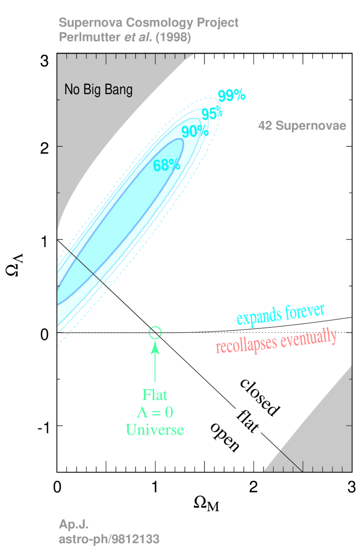
Figure 2.7: The best fit to the $m(z)$ function for the supernovae data of Perlmutter et al., (1998b). the confidence regions do nothing for determining $\Omega_{0}$ and $\Omega_{\Lambda_{0}}$.

We can see in this figure that their best fit regions do not provide any substantial constraint on $\Omega_{0}$ and $\Omega_{\Lambda_{0}}$, but they do provide quite good constraints in $q_{0}$.

At high redshift a very similar thing happens, but in a less obvious way. The series expansion of the $m(z)$ curve is clearly useless for any intuitive idea of what’s going on. However, if we consider the CMB to have an intrinsic and apparent magnitude, then we can examine the exact $m-z$ relation at $z=1000$ and plot the contours of constant $m$ on the $\Omega_{0}-\Omega_{\Lambda_{0}}$ phase plane. See Fig. 2.8, where $m-M-25$ is plotted in the $\Omega_{0}-\Omega_{\Lambda_{0}}$ plane, with contours of constant $m-M-25$ marked on it. In practice we can calculate $m-M-25$ for any object from observations (giving $m$) and assumptions about the objects intrinsic brightness ($M$). Thus we can select just one contour in (2.8), and get some limitations on $\Omega_{0}$ and $\Omega_{\Lambda_{0}}$. Just as in the SNIa results, the constraints will be weak, with any particular contour selecting a large range of allowed values for $\Omega_{0}$ and $\Omega_{\Lambda_{0}}$ (unless $\Omega_{0}$ is small). It should be noted that this is a very simple analysis, because the degeneracy of the CMB in the $\Omega_{0}-\Omega_{\Lambda_{0}}$ plane comes from the position of the first Doppler peak (cf, figure 1.2) rather than simply the $m-z$ relation, but the principle is the same.

Tegmark et al. have noticed that when the results from the CMB are taken together with the SNIa results, then it is possible to get very precise predictions of $\Omega_{0}$ and $\Omega_{\Lambda_{0}}$ separately. If we have a look at Fig. 2.8 we can see why.

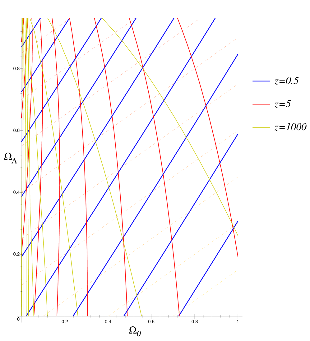
Figure 2.8: The phase diagram for the $m-z$ relation for $z=0.5,5,1000$ presented in the $\Omega_{0}-\Omega_{\Lambda_{0}}$ plane. We can see that the contours move round the diagram with increasing redshift. The faint dashed lines are constant $q_{0}$, which shows that low redshift observations will give good results for $q_{0}$.

We have plotted contours, as described above, for redshifts of 0.5, 5, and 1000. Typically, a set of observations at low redshift will determine one of the blue contours (obviously this means a set of contours in a small neighborhood of some mean or ‘best fit’ contour); similarly, the CMB measurements will determine a similar set of the yellow contours. Because these contours intersect at a fairly large angle, it is only the overlap of these curves where the real universe will lie (provided the universe is FLRW of course).

For completeness, we show in Fig, 2.9 the results of Tegmark, Eisenstein and Hu (1998a) who computed this overlap for future SNIa and CMB observations.

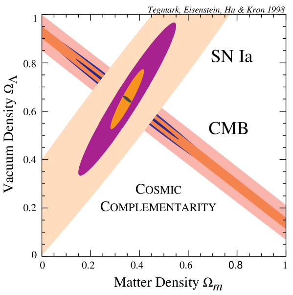
Figure 2.9: A futureistic diagram of what might be expected from SNIa and CMB complementing each other in the future. The errors on $\Omega_{0}$ and $\Omega_{\Lambda_{0}}$ (small black ellipse) are extremely small (by cosmology standards) in comparison with the independent results. Plagiarised from Tegmark, Eisenstein and Hu (1998a).

We also show another stolen picture, Fig, 2.10, which gives the same sort of results as Fig, 2.8, but for number-counts, age and growth as well.

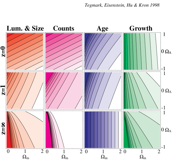
Figure 2.10: Extra results similar to (2.8) for other number-counts, age and growth as well. From Tegmark et al., (1998b).

What is also interesting about figure 2.8 is something that none of the papers above have mentioned; a quick look at the figure shows the contours chang angle from $\sim 45^{\circ}$ to $>90^{\circ}$. This means that there will be some redshift ($z\sim 3$) for which the lines will be vertical; ie, $\Omega_{0}$ will be determined to very high accuracy from just one set of experiments independent of $\Omega_{\Lambda}$. In fact it may be worth specifically looking for eg, quasars or SNIa at this redshift to give a very accurate determination of $\Omega_{0}$ (and hence $\Omega_{\Lambda_{0}}$ from other redshift surveys).

2.9 Observable Quantities in a General Spacetime

In the FLRW models, there is a simple relation between the fundamental length scale $a$ and the observable parameters $H_{0},q_{0}$ etc. It is interesting to determine the correct covariant definitions of $H_{0}$ and $q_{0}$ for a general cosmological model and to ask whether the FLRW $\Omega_{\Lambda}$ generalises to other cosmological models. Almost invariably these parameters are measured fitting distance-redshift data to an FLRW model (essentially eq. (2.4)). What can this say about other inhomogeneous models; and what could be causing a negative $q_{0}$ other than a cosmological constant?

The standard generalisations of $H_{0}$ and $q_{0}$ are based on the fundamental length scale defined by (2.17) simply by generalising the definitions for FLRW models, (2.119) and (2.120), viz;

$$H \!\!\!\!= \!\!\!\!{\frac{\dot{\ell}}{\ell}}\equiv{\frac{1}{3}}\theta;$$ (2.152)

$$q \!\!\!\!= \!\!\!\!-{\frac{\ddot{\ell}\ell}{\dot{\ell}^{2}}}.$$ (2.153)

Using the Raychaudhuri equation (2.37) we find simply that

$$q={\frac{1}{2}}\Omega\left(1+{\frac{p}{\mu}}\right)-\Omega_{\Lambda}+{\frac{1}{H}}\left(2(\sigma^{2}-\omega^{2})-{\frac{1}{3}}\left[\widetilde{\nabla}_{a}\dot{u}^{a}+\dot{u}^{2}\right]\right).$$ (2.154)

(See eq. (52) in Ellis, 1998. Note that his statement about the acceleration terms being small from CMB anisotropies is false – see Chapter 3.)

The definition of the expansion $\theta$ is the volume change along $u^{a}$: defining $H$ via (2.152) is misleading. It gives the average distance change to neighbouring particles along $u^{a}$; whereas the actual distance change to a particle in direction $e^{a}$ is given by

$${\frac{(\delta\ell)^{\cdot}}{\delta\ell}}={\textstyle\frac{1}{3}}\theta+\sigma_{ab}e^{a}e^{b}=H;$$ (2.155)

as one would expect, the shear will affect the distance to neighbouring particles, as some may be moving towards or away from you relative to the overall expansion – see Ehlers (1993). Now this is a good definition of the Hubble scalar, and has been used before. Often, the expansion tensor is defined as (eg, Wainwright and Ellis 1997)

$$\Theta_{ab}\!\!\mathrel{\vbox{\hbox{ \ooalign{\raise 4.75pt\hbox{${\textsf{\tiny{\,def}}}$}\crcr$=$}}}}\sigma_{ab}+{\textstyle\frac{1}{3}}\theta h_{ab}$$ (2.156)

so we can now define

$$H\!\!\mathrel{\vbox{\hbox{ \ooalign{\raise 4.75pt\hbox{${\textsf{\tiny{\,def}}}$}\crcr$=$}}}}\Theta_{ab}e^{a}e^{b}$$ (2.157)

to give a covariant, direction-dependent definition of the Hubble scalar. This has been used in Humphreys et al. (1997).

If we want to compare a non-standard cosmological model with the real universe (or with an FLRW model, with values of $H_{0}$ etc. derived from them) then we need a generalisation of $H_{0}$ and $q_{0}$ suitable for a decent comparison with data. It has been suggested that equating the various order terms in the generalised $m-z$ series relation with those of the FLRW series would give the proper generalised $H_{0}$ and $q_{0}$ (Humphreys et al. 1997; Paczyński and Piran 1990; Domínguez-Tenreiro 1981a,b; also see Palle 1999). So, comparing (2.110) with (2.151) we can define

$$\left.H^{{}^{\tiny{\textsf{obs}}}}\right|_{0} \!\!\!\!\!\!\mathrel{\vbox{\hbox{ \ooalign{\raise 4.75pt\hbox{${\textsf{\tiny{\,def}}}$}\crcr$=$}}}} \!\!\!\!\left.K^{a}K^{b}\nabla_{a}u_{b}\right|_{0},$$ (2.160)

$$\left.q^{{}^{\tiny{\textsf{obs}}}}\right|_{0} \!\!\!\!\!\!\mathrel{\vbox{\hbox{ \ooalign{\raise 4.75pt\hbox{${\textsf{\tiny{\,def}}}$}\crcr$=$}}}} \!\!\!\!\left.{\frac{K^{a}K^{b}K^{c}\nabla_{a}\nabla_{b}u_{c}}{(K^{d}K^{e}\nabla_{d}u_{e})^{2}}}\right|_{0}-3.$$ (2.163)

Expanding $H^{{}^{\tiny{\textsf{obs}}}}$ gives

$$H^{{}^{\tiny{\textsf{obs}}}}_{0}=\underbrace{{\textstyle\frac{1}{3}}\theta}_{\mathsf{monopole}}+\underbrace{\dot{u}_{a}e^{a}}_{\mathsf{dipole}}+\underbrace{\sigma_{ab}e^{a}e^{b}}_{\mathsf{quadrupole}};$$ (2.164)

where the quantities on the right hand side are understood to be evaluated at the present time. This definition does not have the physical significance of (2.157); rather it is the zero point of the linear Hubble relation. To compare a non-standard model to an FLRW model at low redshift, then (2.164) is the definition which must be used. Eq, (2.164) shows that a general inhomogeneous cosmological model has the effect of inducing a dipole and quadrupole in the $m-z$ relation as $z\rightarrow 0$. However, this conclusion only concerns measurements made at very small redshift, say $z\mathrel{\vbox{\hbox{\tiny\ooalign{\raise 3.25pt\hbox{$<$}\crcr$\sim$}}}}0.1$, because, as we have seen in §2.8.1, we cannot be sure that the low-order terms in the series expansion will give a function even approximating the real thing for larger redshift (say, $z\mathrel{\vbox{\hbox{\tiny\ooalign{\raise 3.25pt\hbox{$>$}\crcr$\sim$}}}}0.1$). In other words, at higher redshifts (eg, for SNIa) higher order terms may modify these moments to some degree.

All of these low redshift surveys essentially use the linear Hubble Law which, for a general cosmological model reads

$$z=\left.K^{a}K^{b}\nabla_{a}u_{b}\right|_{0}r_{A}+{\cal{O}}(r_{A}^{2})=H^{{}^{\tiny{\textsf{obs}}}}_{0}r_{A}+{\cal{O}}(r_{A}^{2}).$$ (2.165)

If we write this in the more suggestive form

$$z\simeq H_{0}r\left(1+{\frac{\dot{u}_{a}e^{a}}{H_{0}}}+{\frac{\sigma_{ab}e^{a}e^{b}}{H_{0}}}\right),$$ (2.166)

where $H_{0}$ is the expansion rate (2.152) as in the FLRW models (basically the all sky average expansion rate) Equation (2.166) reflect the effects of local small-scale inhomogeneities, ie, perturbations of the smooth background model. If we and add in these local effects, (this is often done in terms of spherical harmonics, eg, Regös and Szalay 1989; or Branchini et al. (1999); Tadros et al. 1999 – but we shall just use $\cos\vartheta$ expansion) represented by constants $b_{1},b_{2},b_{3}\cdots$, we have

$$z\simeq H_{0}r\left(1+{\frac{\dot{u}_{a}e^{a}}{H_{0}}}+{\frac{\sigma_{\langle ab\rangle}e^{a}e^{b}}{H_{0}}}\right)+b_{1}\cos\vartheta+b_{2}r\cos\vartheta+b_{3}r\cos^{2}\vartheta+\cdots,$$ (2.167)

where $r_{A}$ has been replaced by $r$ because all definitions of $r$ agree at very small redshift. $b_{1}$ corresponds to the bulk flow of the local group moving relative to the CMB frame, and $b_{3}$ often corresponds to a shearing effect from our infall to the Great Attractor and Virgo cluster – see eg, Lilje, Yahil and Jones (1986) who first reported the effect. However, there is no physical local effect that will produce $b_{2}\neq 0$. It is certainly not clear at all that $b_{2}=0$ on observational grounds; this leaves acceleration as the only effect that will produce a dipole in the Hubble law which grows linearly with distance.

If we try to determine from equation (2.167) from galaxy surveys then we must be able to determine how much of the observed dipole is bulk flow and how much may be attributed to any possible acceleration term; ie, whether any of the dipole grows with distance. In principle we may be able to limit the acceleration quite strongly in this way. However, preliminary results using the IRAS catalogue only constrain

$${\frac{\left\langle\dot{u}_{a}e^{a}\right\rangle_{{}_{\mathsf{half~{}sky}}}}{H_{0}}}<0.2.$$ (2.168)

(Clarkson, Rauzy and Barrett, in preparation.) This is not strict at all, but it is likely that a more complete survey such as the PSCz catalogue may provide stronger constraints.

The generalised $q^{{}^{\tiny{\textsf{obs}}}}_{0}$ is not nearly so simple; expanding (2.163), and substituting for $\dot{\theta}$, $\dot{\sigma}_{\langle ab\rangle}$ and $\widetilde{\nabla}_{b}\sigma^{ab}$ from (2.37), (2.40) and (2.44) respectively we find

$$\begin{array}[]{ll|c}q^{{}^{\tiny{\textsf{obs}}}}_{0}&\!\!\!\!={H^{{}^{\tiny{\textsf{obs}}}}_{0}}^{-2}\left\{{\textstyle\frac{1}{6}}\mu+{\textstyle\frac{1}{2}}p-{\textstyle\frac{1}{3}}\Lambda-{\textstyle\frac{2}{3}}\widetilde{\nabla}_{a}\dot{u}^{a}+{\textstyle\frac{6}{5}}\sigma^{2}-{\textstyle\frac{2}{3}}\omega^{2}\right.&\mathsf{monopole}\\ &\left.+e^{a}\left[-{\textstyle\frac{2}{3}}\theta\dot{u}_{a}-{\textstyle\frac{3}{5}}\widetilde{\nabla}_{a}\theta-\ddot{u}_{a}+\dot{u}^{b}\sigma_{ab}+{\textstyle\frac{2}{5}}q_{a}\right.\right.&\\ &\hfill\left.\left.+{\textstyle\frac{3}{5}}\eta_{a}^{\phantom{h}bc}\left(\widetilde{\nabla}_{b}\omega_{c}+2\dot{u}_{b}\omega_{c}\right)\right]\right.&\mathsf{dipole}\\ &\left.+e^{a}e^{b}\left[-2\widetilde{\nabla}_{\langle a}\dot{u}_{b\rangle}+\dot{u}_{\langle a}\dot{u}_{b\rangle}+E_{\langle ab\rangle}-{\textstyle\frac{1}{2}}\pi_{\langle ab\rangle}+{\textstyle\frac{9}{7}}\sigma^{\vphantom{c}}_{c\langle a}\sigma_{b\rangle}^{\phantom{b\rangle}c}\right.\right.&\\ &\hfill\left.\left.+\omega_{\langle a}\omega_{b\rangle}-{\textstyle\frac{2}{3}}\sigma^{\vphantom{c}}_{c\langle a}\omega_{b\rangle}^{\phantom{b\rangle}c}\right]\right.&\mathsf{quadrupole}\\ &\hfill\left.+e^{a}e^{b}e^{c}\left[-5\dot{u}_{\langle a}\sigma_{bc\rangle}-\widetilde{\nabla}_{\langle a}\sigma_{bc\rangle}\right]-3e^{a}e^{b}e^{c}e^{d}\sigma_{\langle ab}\sigma_{cd\rangle}\right\}.&\mathsf{higher\phantom{h}multipoles}\end{array}$$

This is somewhat complicated for an observable quantity. Measurements of $q_{0}$ are nowhere near accurate enough to detect any multipole moments; in fact it is only recently that the sign of the deceleration parameter has been decided upon, let alone a variation in the sky. However, if we consider the mean value of (2.9) around the sky, then we have

$$\left\langle{H^{{}^{\tiny{\textsf{obs}}}}}^{2}q^{{}^{\tiny{\textsf{obs}}}}\right\rangle_{{}_{\mathsf{all~{}sky}}}={\textstyle\frac{1}{6}}\mu+{\textstyle\frac{1}{2}}p-{\textstyle\frac{1}{3}}\Lambda-{\textstyle\frac{2}{3}}\widetilde{\nabla}_{a}\dot{u}^{a}+{\textstyle\frac{6}{5}}\sigma^{2}-{\textstyle\frac{2}{3}}\omega^{2},$$ (2.169)

which, we can compare to the definition given by the length scale (2.154):

$$\left\langle H^{2}q\right\rangle_{{}_{\mathsf{all~{}sky}}}={\textstyle\frac{1}{6}}\mu+{\textstyle\frac{1}{2}}p-{\textstyle\frac{1}{3}}\Lambda-{\textstyle\frac{1}{3}}\widetilde{\nabla}_{a}\dot{u}^{a}-{\textstyle\frac{1}{3}}\dot{u}_{a}\dot{u}^{a}+2(\sigma^{2}-\omega^{2}).$$ (2.170)

We find that the shear and rotation become less important in the observationally derived relation, while the acceleration terms become relatively more important. More interestingly though is the contribution from the acceleration vector $\dot{u}^{2}$, has disappeared: it will actually contribute nothing to the value of the deceleration.

Chapter 3 The Ehlers-Geren-Sachs Theorem and Some Generalisations

The high isotropy of the CMB is usually taken as strong evidence that the universe is homogeneous and isotropic, ie, is well described by an FLRW model. The principle justification for this is an important theorem of Ehlers, Geren and Sachs (1968) (based on earlier work by Tauber and Weinberg 1961), which states that if all observers in an expanding, dust universe measure an isotropic CMB then the universe is FLRW and the cosmological principle is valid. The importance of this theorem lies in the fact that it permits the homogeneity and isotropy of the universe to be deduced not from measurements of the actual isotropy of the universe about us, but from only measurements of the CMB, combined with the Copernican principle (that is, the assumption that all observers in the universe see the same degree of isotropy). The Copernican principle is often regarded as a powerful but untestable assumption in cosmology, although there are suggestions that it may be testable using the Sunyaev-Zeldovich effect, for example (Goodman 1995). Here we simply assume that the Copernican principle is valid and study the consequences of applying it to the observed high degree of isotropy of the CMB. That is, we examine spacetimes with an isotropic CMB for all observers.

The EGS theorem has been generalised by Treciokas and Ellis (1971) to include an isotropic collision term. Ferrando, Morales, and Portilla (1992) find the general form of the energy-momentum tensor and Einstein’s equations for spacetimes with an isotropic radiation field, and consider some special cases with anisotropic pressure. It has also been shown by Stoeger, Maartens and Ellis (1995) that the EGS theorem almost holds when applied to an almost isotropic radiation field.

There are counterexamples to the spirit of the EGS theorem (that is, when some of the assumptions are relaxed the result fails to hold). In particular, Ellis, Maartens and Nel (1978) show that the result does not hold if the expansion is zero (which is obviously not relevant to cosmology), and Ferrando et al. (1992) emphasise that homogeneity does not follow if there is anisotropic pressure in the energy-momentum tensor. Nilsson et al. (1999) provide a counterexample to the almost EGS result when the Weyl curvature is not negligible.

The basis of the EGS theorem is the Liouville equation for photons, which tells us that if a radiation field (ie, a solution of the Liouville equation) exists such that for every observer on some timelike congruence the radiation field is isotropic, then that congruence is (parallel to) a conformal Killing vector (CKV). This may be expressed more formally as follows (Ehlers et al. 1968; Ferrando et al. 1992):

Theorem 1

A spacetime will admit an isotropic radiation field if and only if it is conformal to a stationary spacetime, which happens if and only if there is a velocity field $u^{a}$ satisfying

$$\sigma_{ab}=0,$$ (3.1)

$$\nabla_{[a}\left(\dot{u}_{b]}-{\textstyle\frac{1}{3}}\theta u_{b]}\right)=0,$$ (3.2)

where $\sigma_{ab}$, $\dot{u}^{a}$ and $\theta$ are the shear, acceleration and expansion of $u^{a}$, respectively.

(Then $u^{a}$ is the velocity field relative to which the radiation is isotropic, and is parallel to the CKV.)

The proof of Theorem 1 is very straightforward in the 1+3 formalism, and follows from the results of §2.6 and §2.3 in Chapter 2.

Proof

With reference to §2.6 a radiation field is isotropic (with respect to $u^{a}$) iff $q_{\!{}_{R}}^{a}\equiv\pi_{\!{}_{R}}^{ab}\equiv\Pi_{A_{\ell}}=0~{}\forall~{}\ell>2$, and from (2.87)-(2.89) we find that this condition implies

$$\dot{\mu}_{\!{}_{R}}+{\frac{4}{3}}\theta\mu_{\!{}_{R}} \!\!\!\!= \!\!\!\!0$$

$$4\mu_{\!{}_{R}}\dot{u}_{a}+\widetilde{\nabla}_{a}\mu_{\!{}_{R}} \!\!\!\!= \!\!\!\!0$$

$$\sigma_{ab} \!\!\!\!= \!\!\!\!0.$$ (3.3)

Now, if we write $Q\!\!\mathrel{\vbox{\hbox{ \ooalign{\raise 4.75pt\hbox{${\textsf{\tiny{\,def}}}$}\crcr$=$}}}}-{\textstyle\frac{1}{4}}\ln\mu_{\!{}_{R}}$ in the first two conditions of (3.3) we find that

$$\theta=3\dot{Q},~{}~{}~{}\dot{u}_{a}=\widetilde{\nabla}_{a}Q:~{}~{}~{}\Longleftrightarrow~{}~{}~{}\nabla_{[a}\left(\dot{u}_{b]}-{\textstyle\frac{1}{3}}\theta u_{b]}\right)=0;$$ (3.4)

which, together with (2.50) and $\sigma_{ab}=0$, tells us that the spacetime is conformally stationary $\hat{\theta}=\hat{\dot{u}}^{a}=\hat{\sigma}_{ab}=0$.$\hfill\Box$

In the absence of some statement about the matter content of a spacetime, or further assumptions about the congruence $u^{a}$, Theorem 1 is all that can be said. In a cosmological context the simplest, and most common, assumption is that the matter is dust (implying that $u^{a}$ is geodesic), which leads to:

Theorem 2 (Ehlers, Geren, and Sachs)

If the fundamental observers in a dust spacetime see an isotropic radiation field, then the spacetime is locally FLRW.

Proof:

This is a straight forward extension of the proof of Theorem 1: we have for a dust congruence $\dot{u}^{a}\equiv 0$ which implies $\widetilde{\nabla}_{a}Q=0$. Now, by (2.22) we find for $\theta\neq 0$ that $\dot{Q}\omega_{ab}=0$: hence the spacetime is a perfect fluid with geodesic, irrotational, shear-free flow, and is therefore an FLRW model (see Krasiński 1997).$\hfill\Box$

Alternatively, we can simply assume that $u^{a}$ is geodesic. The existence of an isotropic radiation field then ensures (for non-zero expansion) that the energy flux relative to $u^{a}$ is zero. If the anisotropic stress tensor is zero at any instant (so that the energy-momentum tensor has perfect fluid form) then it will remain zero and the spacetime will be FLRW (Ferrando et al. 1992, Corollary 1; but note that their statement that the anisotropic stress is invariant along $u^{a}$ in general is misleading – from Eqs. (31) and (40) of Ellis 1998 we have $\dot{\pi}_{\langle ab\rangle}\propto\theta\pi_{ab}$).

It is worth emphasising that in applications of the above results to cosmology the motion of the fundamental observers must be identified with the congruence $u^{a}$. For example, in §3.1.2 all Stephani models are conformally flat, and therefore conformally stationary, but for most of these spacetimes the fluid congruence is not aligned with the timelike CKV.

The matter content of the universe is not precisely known. Certainly, there is a large number of possible contributors, including hot and cold dark matter (in their various manifestations), electromagnetic fields etc., as well as the more obvious radiation and baryonic matter. In particular, the type Ia supernova results of Perlmutter et al. (1999) suggest that an important component may be a ‘quintessential’ scalar field. However, the forms of matter that are thought to contribute significantly to the energy-momentum tensor may be treated in general as perfect fluids. That is, their energy-momentum tensor may be written in the form

$$T_{ab}=\mu u_{a}u_{b}+ph_{ab},$$ (3.5)

where $\mu$ and $p$ are the energy density and pressure, $u^{a}$ is the timelike velocity congruence of the fluid, and $h_{ab}$ is the spatial projection tensor associated with $u^{a}$. Scalar fields may also be written in this form, with $u^{a}$ parallel to the gradient of the scalar field, provided that this is timelike (see §3.2). Note that if several such components are present there is no reason why their fundamental congruences (the $u^{a}$’s) should be parallel. If they are, then they may be treated as effectively a single perfect fluid with the energy densities and pressures added together. If not, the decomposition of the energy-momentum with respect to $u^{a}$ for one such fluid (as in equation (14) of Ellis 1998) will contain energy flux and anisotropic stress terms from the other fluids (again, see §3.2). The fundamental observers will be associated with one such congruence. Usually the fundamental observers in standard models of the universe are associated with a dust-like ($p=0$) component, with the result that the acceleration $\dot{u}^{a}$ of the fundamental congruence is zero. However, we wish to study the consequences of relaxing this assumption and consider models with acceleration. This acceleration must be caused by some non-gravitational force (typically pressure gradients for perfect fluid spacetimes, but in principle it could be the result of a coupling between the fluid and some other component such as the electromagnetic field).

With this in mind, in this paper we consider perhaps the two simplest generalisations of the dust hypothesis. Firstly we imagine that the dominant form of matter is a single irrotational perfect fluid. We do not specify what form of matter this corresponds to, but we allow pressure gradients that give rise to acceleration. Secondly we consider cosmological models in which more than one matter component makes a significant contribution to the energy density and dynamics of the universe. Specifically we consider ‘QCDM’ models, containing a non-interacting mixture of radiation, dust (CDM) and a scalar field (or a cosmological constant). The observers are associated with the CDM component, and are therefore geodesic. The difference between this and other theorems assuming geodesic observers is that the the scalar field component can introduce effective energy flux and anisotropic stresses relative to the dust congruence, and so the matter need not behave as a perfect fluid.

In the following section we find all irrotational perfect fluid solutions admitting an isotropic radiation field for the fundamental observers, showing that they form a subclass of the Stephani spacetimes and are FLRW if and only if the acceleration vanishes. Then in §3.2 we examine QCDM models and prove that such models must be homogeneous and isotropic if they admit an isotropic radiation field. Finally, in §3.3 we emphasise the importance of acceleration for these results and show that the acceleration of the fundamental congruence is, in principle, detectable, and measureable, in galaxy surveys. Two appendices contain results relating to §3.1.2.

3.1 The Irrotational Perfect Fluid Solutions.

We wish to consider the constraints imposed by the existence of an isotropic radiation field for the fundamental observers on perfect fluid spacetimes in which the rotation of the fundamental congruence is zero. Since it follows from Theorem 1 that the shear of the fundamental congruence must also be zero we immediately know that all the acceptable solutions are members of the Stephani-Barnes family, which is the family of all shear-free, irrotational, expanding (or contracting) perfect fluids (see Krasiński 1989, 1997). It only remains, then, to impose condition (3.2) of Theorem 1 and thus find the sub-class of Stephani-Barnes models which admit an isotropic radiation field for all fundamental observers.

The Stephani-Barnes family contains the Barnes solutions, which are of Petrov type D, and the Stephani models, which are conformally flat, although these two classes overlap where the Barnes solutions degenerate to type O (these solutions then become Stephani models with symmetry). The FLRW models are a subcase of these solutions. The Barnes spacetimes all possess symmetry (see below), whereas the Stephani spacetimes, in general, do not. In all cases the metric in comoving coordinates can be written in the form (we use the same notation as Krasiński 1997):

$$ds^{2}=V^{-2}\left\{-(FV_{,t})^{2}dt^{2}+dx^{2}+dy^{2}+dz^{2}\right\}$$ (3.6)

where $F=F(t)$ and $V=V(t,x,y,z)$. $F(t)$ is arbitrary, but there are some restrictions on the form of $V$ depending on the symmetries of the solution, and these will be discussed in due course (but the impatient reader may wish to note Eqs. 3.12, 3.14, 3.15, and 3.17). Expressions for the energy density and pressure can be found in Krasiński (1997).

The fluid velocity is given by (without loss of generality we can assume that $V>0$)

$$u^{a}=\frac{V}{|FV_{,t}|}\delta^{a}_{\phantom{a}0},$$ (3.7)

with expansion

$$\theta=-\hbox{sign}(V_{,t})\frac{3}{|F|},$$ (3.8)

and acceleration

$$\dot{u}_{0}=0,\hskip 28.45274pt\dot{u}_{i}=\frac{\partial}{\partial x^{i}}\ln\frac{V_{,t}}{V},$$ (3.9)

where $i=1,2,3$, $x^{i}=\{x,y,z\}$. Note that (3.8) differs from the expression usually given for the expansion (in Krasiński 1997, equations (4.1.4) and (4.9.6), for example) by the inclusion of the $-\hbox{sign}(V_{,t})$ factor. Neglect of this factor is inconsistent since $F$ enters the metric only quadratically, so the sign of the expansion cannot depend on the sign of $F$. The sign of $\theta$ does depend on that of $V_{,t}$, though: for the Friedmann subcase of the Stephani-Barnes models, for example, $V$ is related to the scale factor $R(t)$ by $V=1/R$, and $|FV_{,t}/V|=1$ (see §3.1.2), so that $\theta=3\dot{R}/R=-3V_{,t}/V=-3\,\hbox{sign}(V_{,t})/|F|$. This is important here because the constraint (3.2) contains the expansion. Note, too, that $F$ is not a true degree of freedom parameterising distinct spacetimes, but rather represents a coordinate freedom, corresponding to different choices of the time coordinate.

From (3.7), (3.8) and (3.9), the condition (3.2) leads to the constraint:

$$\frac{\partial^{2}}{\partial x^{i}\partial t}\ln V_{,t}=0,$$ (3.10)

which is satisfied if and only if the function $V$ has the form

$$V(t,x,y,z)=T(t)X(x,y,z)+Y(x,y,z),$$ (3.11)

where $T$, $X$, and $Y$ are arbitrary functions. This equation is the key additional constraint on the Stephani-Barnes solutions.

It is worth noting that it follows from (3.10) that the acceleration scalar is constant along the fluid flow for every observer, ie, $\dot{u}_{,t}=0$ (where $\dot{u}^{2}=\dot{u}_{a}\dot{u}^{a}$), as can be seen by calculating $(\dot{u}^{2})_{,t}$ from (3.9). In fact, it can be verified more generally that for any conformally stationary spacetime (ie, a spacetime satisfying (3.1) and (3.2)), even with rotation, the acceleration scalar evolves according to

$$u^{a}\nabla_{a}\dot{u}^{2}={\textstyle\frac{2}{3}}\dot{u}^{b}\widetilde{\nabla}_{b}\theta,$$

where $\widetilde{\nabla}$ denotes the spatially projected gradient (see Ellis 1998). It follows from equation (32) of Ellis (1998) that $\widetilde{\nabla}_{b}\theta=0$ whenever the rotation vanishes (for a perfect fluid), which is the case for the Stephani-Barnes models.

Note that if $V$ has the form (3.11) we can immediately write the metric in a manifestly conformally static form

$$ds^{2}=\frac{X^{2}}{V^{2}}\left\{-d\tau^{2}+X^{-2}(dx^{2}+dy^{2}+dz^{2})\right\},$$

where $d\tau=T_{,t}F\,dt$, which shows that these models will indeed be conformally stationary, as required by Theorem 1. We now discuss each subcase in turn.

3.1.1 The Barnes Solutions.

The Barnes solutions all have spherical, plane or hyperbolic symmetry (ie, they possess three-dimensional isometry groups acting on two-dimensional orbits, cf. §3.1.2). The restrictions on the metric function $V$ depend on which of these symmetries the spacetime possesses (see Krasiński 1997). For the solutions with spherical symmetry (the Kustaanheimo-Qvist solutions) or planar symmetry we introduce a new independent variable $u(x,y,z)$ defined by $u=r^{2}=x^{2}+y^{2}+z^{2}$ in the spherical case and $u=z$ in the planar case. Then $V$ is defined by $V=V(t,u)$, subject to the condition:

$$\frac{\partial^{2}V}{\partial u^{2}}=f(u)V^{2}.$$ (3.12)

where $f$ is an arbitrary function. Since $V=V(t,u)$ we know from (3.11) that in order to admit an isotropic radiation field for all observers $V$ must have the form

$$V(t,u)=T(t)X(u)+Y(u).$$ (3.13)

Equation (3.12) then imposes a constraint on the functions $X$ and $Y$, which will be outlined below.

For the solutions with hyperbolic symmetry the constraint on $V$ is very similar. This time we introduce the variable $u=x/y$. $V$ can then be written

$$V(t,x,y)=yW(t,u),$$ (3.14)

where $W$ satisfies

$$\frac{\partial^{2}W}{\partial u^{2}}=f(u)W^{2},$$ (3.15)

with $f$ once again a free function. The condition (3.11) now gives

$$V(t,x,y)=T(t)X(x,y)+Y(x,y)=yW(t,u).$$

Dividing by $y$ and redefining $X$ and $Y$ in an obvious fashion we obtain

$$W(t,u)=T(t)\tilde{X}(u)+\tilde{Y}(u),$$ (3.16)

in which $\tilde{X}$ and $\tilde{Y}$ are again constrained by (3.15).

For all three symmetries of the Barnes solutions, then, the constraints on the metric function $V$ essentially reduce to the second-order differential equations (3.12) or (3.15). Imposing the condition (3.11) introduces the additional constraint (3.13) or (3.16). Substitution of (3.13) or (3.16) into (3.12) or (3.15) respectively and differentiating twice with respect to time, dividing by $T_{,t}$ each time (and recognising that $T_{,t}\neq 0$, $X\neq 0$, so that $V_{,t}\neq 0$ in (3.6)), leads directly to the condition

$$f(u)=0.$$

Barnes solutions with $f(u)=0$ are conformally flat (Krasiński 1997, p.142) and are therefore actually a subcase of the Stephani models. That is, proper Barnes spacetimes can be ruled out: they do not admit an isotropic radiation field. It only remains to apply the condition (3.11) to the Stephani models, which we do in the next section.

3.1.2 The Conformally Flat Solutions

The conformally flat sub-case is the entire class of conformally flat, expanding, perfect fluid solutions, and is the Stephani solution (Stephani 1967a,b). The function $V$ is most often written in the form (see Krasiński 1997; Barrett and Clarkson 1999a,b):

$$V(t,x,y,z)=\frac{1}{R(t)}\left(1+{\textstyle\frac{1}{4}}k(t)|{\mathbf{x}}-{\mathbf{x}}_{0}(t)|^{2}\right)$$ (3.17)

In general the five functions of time in $V$ are free. For our purposes, however, it turns out to be more convenient to use

$$V=a(t)+b(t)r^{2}-2{\mathbf{c}}(t)\cdot{\mathbf{r}},$$ (3.18)

as in Barnes (1998), again with five free functions (we adopt three-dimensional vector notation, so that ${\mathbf{c}}=(c_{1},c_{2},c_{3})$, for example). In fact, this form is slightly more general than (3.17) – see Barnes (1998).

We must be able to write $V$ in the form (3.11) for the spacetime to admit an isotropic radiation field for all fundamental observers. From (3.17) or (3.18) it is clear that the functions $X(x^{i})$, and $Y(x^{i})$ in (3.11) can be at most quadratic in the $x^{i}$. Writing $X$, and $Y$ as quadratics in (3.11) and equating in (3.18) all powers of $x^{i}$, we obtain the following constraint equations:

$$a(t) \!\!\!\!= \!\!\!\!a_{1}T(t)+a_{2},$$

$$b(t) \!\!\!\!= \!\!\!\!b_{1}T(t)+b_{2},$$ (3.19)

$${\mathbf{c}}(t) \!\!\!\!= \!\!\!\!{\mathbf{c}}_{1}T(t)+{\mathbf{c}}_{2},$$

where $T(t)$ is a free function of time and the $a_{1,2}$, $b_{1,2}$ and ${\mathbf{c}}_{1,2}$ are ten independent constants. Not all of $a_{1}$, $b_{1}$ and ${\mathbf{c}}_{1}$ can be zero (in order that $V,_{t}\neq 0$ in (3.6)).

Equations (3.19), along with (3.6) and (3.18), provide the complete set of irrotational perfect fluid spacetimes admitting an isotropic radiation field. Not all of the possible choices of parameters give rise to distinct spacetimes, though, and we outline in appendix A how coordinate transformations may be used to eliminate many of the parameters in (3.19), and determine when the models can be reduced to manifestly spherically symmetric form (${\mathbf{c}}={\mathbf{0}}$).

The Constraints on $R$, $k$ and ${\mathbf{x}}_{0}$.

To find the constraints on $R$, $k$ and ${\mathbf{x}}_{0}$ in (3.17) corresponding to (3.19) first equate powers of $x^{i}$ in (3.17) and (3.18) to obtain

$$a(t) \!\!\!\!= \!\!\!\!\frac{1}{R}+\frac{k}{4R}|{\mathbf{x}}_{0}|^{2},$$ (3.20)

$$b(t) \!\!\!\!= \!\!\!\!\frac{k}{4R},$$ (3.21)

$${\mathbf{c}}(t) \!\!\!\!= \!\!\!\!\frac{k}{4R}{\mathbf{x}}_{0}.$$ (3.22)

Solving these equations for $R$, $k$ and ${\mathbf{x}}_{0}$ gives

$$R(t) \!\!\!\!= \!\!\!\!\frac{b}{ab-|{\mathbf{c}}|^{2}},$$ (3.23)

$$\frac{1}{4}k(t) \!\!\!\!= \!\!\!\!\frac{b^{2}}{ab-|{\mathbf{c}}|^{2}},$$ (3.24)

$${\mathbf{x}}_{0} \!\!\!\!= \!\!\!\!\frac{\mathbf{c}}{b},$$ (3.25)

which are valid whenever ${ab-|{\mathbf{c}}|^{2}}\neq 0$ (otherwise $V$ cannot be written in the form (3.17)).

To impose the constraints (3.19) perform the transformations of appendix A so that ${\mathbf{c}}=c{\mathbf{\hat{z}}}$ as in A.3) and $a_{1}\neq 0$. Then $|{\mathbf{c}}|^{2}=c^{2}$, and $b$ and $a$ are related by

$$b=\frac{b_{1}}{a_{1}}a+\left(b_{2}-\frac{b_{1}a_{2}}{a_{1}}\right)\equiv\gamma a+\delta,$$ (3.26)

where $\gamma=b_{1}/a_{1}$ and $\delta=b_{2}-b_{1}a_{2}/a_{1}$ are constants. Using this in (3.23) and (3.24) leads, after some rearrangement, to a quadratic relationship between $k$ and $R$:

$$\left(\frac{k}{4}\right)^{2}-(\gamma+\delta R)\left(\frac{k}{4}\right)-\gamma c^{2}R^{2}=0.$$ (3.27)

In addition to this constraint relating $k$ and $R$ we can trivially rewrite (3.22) or (3.25) as

$${\mathbf{x}}_{0}=\frac{4R}{k}c{\mathbf{\hat{z}}}.$$ (3.28)

Equations (3.27) and (3.28) are the constraint equations on $R$, $k$ and ${\mathbf{x}}_{0}$ corresponding to the equations (3.19), or rather (A.3). If desired (3.27) can be solved to obtain

$$\frac{k}{4}=\frac{1}{2}\left[\gamma+\delta R\pm\sqrt{(\gamma+\delta R)^{2}+4\gamma c^{2}R^{2}}\right].$$

From (3.27) it is clear that the spherically symmetric Stephani spacetimes admitting an isotropic radiation field, for which $c=0$, satisfy

$$\frac{k}{4}\left(\frac{k}{4}-(\gamma+\delta R)\right)=0,$$

which has the solutions $k=0$ and $R(t)$ free (flat Friedmann), or $k$ linearly related to $R$,

$$\frac{1}{4}k(t)=\gamma+\delta R(t),$$

with $R(t)$ again free (when $\delta=0$ these become Friedmann models with curvature $k=4\gamma$). This fixes notation for the rest of this thesis.

At this point we can say that perfect fluid spacetimes admitting an isotropic radiation field for all fundamental observers are FLRW if and only if the acceleration of the fundamental observers is zero. This follows because the Stephani models with zero acceleration are FLRW (see Krasiński 1997, although it can easily be seen from (3.9): if $\dot{u}=0$ then $V=T(t)X(x^{i})$ for some functions $T$ and $X$, showing that $a$, $b$ and ${\mathbf{c}}$ depend on the single free function $T$ and so must be FLRW by the results of the next section). Thus we have proved:

Theorem 3

The irrotational perfect fluid spacetimes admitting an isotropic radiation field for the fundamental observers are Stephani models with the free functions restricted by (3.19) (or (A.3)). These spacetimes are FLRW if and only if the acceleration of the fundamental observers is zero.

Spacetimes satisfying Theorem 3 will be referred to as IRF models. It is worth noting that all of the models admitting an isotropic radiation field are manifestly conformal to (part of) the Einstein static spacetime (cf. §5.1) once they have been transformed so that ${\mathbf{c}}=c{\mathbf{\hat{z}}}$ as outlined in appendix A. From (3.18) and (A.3) we obtain

$$V_{,t}=a_{1}T_{,t}\left(1+\frac{b_{1}}{a_{1}}r^{2}\right),$$

since ${\mathbf{c}}_{,t}={\mathbf{0}}$ when ${\mathbf{c}}=c{\mathbf{\hat{z}}}$ (as noted in appendix A we can assume $a_{1}\neq 0$). Changing the time coordinate via $dt\mapsto a_{1}T_{,t}F\,dt$, the metric (3.6) becomes

$$ds^{2}=\frac{(1+{\textstyle\frac{1}{4}}\Delta r^{2})^{2}}{V(z,r,t)^{2}}\left\{-dt^{2}+\frac{1}{(1+{\textstyle\frac{1}{4}}\Delta r^{2})^{2}}(dx^{2}+dy^{2}+dz^{2})\right\},$$ (3.29)

where $\Delta=4b_{1}/a_{1}$. The factor in braces is the Einstein static metric. In the following chapter we use this conformal relationship to simplify the study of the observational characteristics of these models.

3.1.3 Symmetry and Thermodynamic Schemes.

Having obtained the conditions (3.19) for a Stephani model to admit an isotropic radiation field it is possible to say immediately that all such spacetimes possess (at least) a three-dimensional symmetry group acting on two-dimensional orbits (just as for the general Barnes models). This follows from the work of Barnes (1998), who showed that the dimension of the isometry group of any Stephani spacetime is determined by the dimension $d$ of the linear space spanned by the five free functions $a$, $b$, and ${\mathbf{c}}$:

1. if $d=4$ or $5$ (ie, at least four of the free functions are linearly independent), then the spacetime has no Killing vectors;

2. if $d=3$ there is a one-dimensional isometry group;

3. if $d=2$ there is a three-dimensional isometry group acting on two-dimensional orbits;

4. if $d=1$ there are six Killing vectors and the spacetime is Robertson-Walker.

It is clear from (3.19) that $a$, $b$, and $\mathbf{c}$ depend on (at most) only two functions of time: $f_{1}(t)=T(t)$ and the constant function $f_{2}(t)\equiv 1$ (since $V_{,t}\neq 0$ we must have $T_{,t}\neq 0$, so that these are necessarily linearly independent). Thus, $d=2$ and the solutions have three-dimensional isometry groups as claimed. If $a_{2}=b_{2}={\mathbf{c}}_{2}=0$ in (3.19) then $d=1$ and the spacetime is FLRW (see appendix A).

It follows further from this and the work of Bona and Coll (1988) (see also Krasiński, Quevedo and Sussman 1997) that all Stephani models that admit an isotropic radiation field for all fundamental observers also admit a strict thermodynamic scheme (that is, entropy and temperature functions can be found that depend on the energy density and pressure and satisfy the second law of thermodynamics). The converse is not true, however, since there are Stephani spacetimes with $d=2$ (which must admit a thermodynamic scheme) that cannot have an isotropic radiation field (these are models for which the second independent function $f_{2}(t)$ is not restricted to be $1$). So, we have the following corollary to Theorem 3:

Corollary 1

An irrotational perfect fluid spacetime that admits an isotropic radiation field has spherical, planar or hyperbolic symmetry and admits a strict thermodynamic scheme.

On the subject of thermodynamics, let us mention for completeness that the thermodynamic scheme occurring most often in the literature is that of a barotropic equation of state. It is known that the only Stephani models with a barotropic EOS are precisely the FLRW models (Bona and Coll 1988; Krasiński 1997). Thus, the only spacetimes with a barotropic EOS admitting an isotropic radiation field are FLRW models. This also follows (when $\mu+p\neq 0$) from a theorem of Coley (1991). See also Collins and Wainwright (1983).

3.2 QCDM Models.

The type Ia supernova results of Riess et al. (1998), Schmidt et al. (1998) and Perlmutter et al. (1999), which suggest that the expansion of the universe is accelerating, have led to an increased interest in cosmological models in which a significant contribution to the energy density comes from either a cosmological constant or a scalar field (quintessence component), which is capable of driving the expansion (Peebles and Ratra 1988; Ratra and Peebles 1988; Caldwell et al. 1998; Zlatev et al. 1999). In QCDM models the matter is an admixture of non-interacting cold dark matter (CDM), ie, dust, and a scalar field. The quintessence component may be thought of as fairies pushing the galaxies apart. The fundamental observers (galaxies) are implicitly identified with the geodesic congruence of the CDM. Note that there is no reason a priori why the scalar field gradient (which defines a natural ‘velocity’ field) should be aligned with the CDM congruence (although it will turn out that they are aligned if the fundamental observers see an isotropic radiation field).

It is interesting to ask whether the EGS theorem can be extended to this case. We demonstrate that it can by proving the following theorem:

Theorem 4

Any solution to Einstein’s equations in which the matter consists of non-interacting radiation, expanding dust (CDM), and a scalar field (or cosmological constant), and for which the dust sees an isotropic radiation field, must either be an FLRW model, or have the gradient of the scalar field orthogonal to the dust congruence.

(Note that the latter possibility means that gradient of the scalar field is spacelike, and is usually rejected as unphysical – although see below.)

Proof:

We may divide this proof into two parts: first we demonstrate from Einstein’s equations in the 1+3 formalism that any energy flux component with respect to the CDM frame must be zero if the CDM observers see isotropic radiation, then we show that the contribution to the energy flux (with respect to the CDM frame) from the scalar field is zero if and only if the gradient of the scalar field is parallel (or orthogonal) to the CDM velocity $u^{a}_{{}_{CDM}}$, so we deduce that the velocity fields are parallel (or orthogonal). The case where the field gradient is orthogonal to $u^{a}_{{}_{CDM}}$ is probably unphysical, and will be rejected. Thus, the mixture of radiation, CDM and scalar field can be written as a single perfect fluid with geodesic fundamental congruence $u^{a}=u^{a}_{{}_{CDM}}$, and it follows from the results of §3.1 that the model is necessarily FLRW.

Since the radiation is isotropic for the dust observers $u^{a}$ the energy-momentum tensor for radiation may be written in the perfect fluid form (3.5) with $p={\textstyle\frac{1}{3}}\mu$ and the total energy-momentum tensor is:

$$T_{ab}=\underbrace{\mu u_{a}u_{b}+{\textstyle\frac{1}{3}}\mu h_{ab}}_{\textrm{Radiation}}+\underbrace{\vphantom{{\textstyle\frac{1}{3}}}\rho u_{a}u_{b}}_{\textrm{CDM}}+\underbrace{\phi_{,a}\phi_{,b}-g_{ab}\left({\textstyle\frac{1}{2}}\phi_{,c}\phi^{,c}+\Phi(\phi)\right)}_{\textrm{Scalar Field}},$$ (3.30)

where $\Phi(\phi)$ is the scalar field potential (often assumed to be zero, in which case the scalar field can be interpreted as a stiff perfect fluid). Note that the cosmological constant case can be included by setting $\phi=\Lambda=$constant, $\Phi(\phi)=\phi$.

1. The fundamental congruence $u^{a}$ is geodesic ($\dot{u}^{a}=0$) because the CDM component does not interact with the other matter. This, in fact, implies that the rotation of $u^{a}$ must also vanish: from the momentum conservation equation for the radiation, we can write

   $$\dot{u}_{a}=-\frac{1}{4}\widetilde{\nabla}_{a}\ln\mu=0$$

   so that (using (2.22))

   $$0=\widetilde{\nabla}_{[a}\dot{u}_{b]}=\frac{1}{4}\widetilde{\nabla}_{[b}\widetilde{\nabla}_{a]}\ln\mu=\frac{1}{4}\omega_{ab}\frac{\dot{\mu}}{\mu}=\frac{1}{3}\omega_{ba}\theta,$$

   and we see that $\omega_{ab}=0$ when $\theta\neq 0$.

   When $\dot{u}_{a}$ and $\omega_{ab}$ are zero, (3.2) becomes

   $$\nabla_{[a}(\theta u_{b]})=u_{[b}\nabla_{a]}\theta=0.$$

   This implies (since $\nabla_{a}\theta=\widetilde{\nabla}_{a}\theta-\dot{\theta}u_{a}$) that

   $$\widetilde{\nabla}_{a}\theta=0.$$ (3.31)

   (ie, the expansion is homogeneous). From the constraint equation relating the divergence of the shear to other kinematical quantities (2.44) we see that any energy flux component with respect to the CDM velocity field must vanish:

   $$q_{a}=\frac{2}{3}\widetilde{\nabla}_{a}\theta=0.$$ (3.32)

   This is the key step in the proof.

2. Decomposing  (3.30) with respect to $u^{a}$ we find that the relative energy flux component is

   $$0=q_{a}=-h_{a}^{~{}b}u^{c}T_{bc}=-\dot{\phi}\widetilde{\nabla}_{a}\phi.$$ (3.33)

   So $q_{a}=0$ if $\dot{\phi}=0$ (the scalar field gradient is orthogonal to $u^{a}$, and therefore spacelike), or if $\widetilde{\nabla}_{a}\phi=0$ (the scalar field gradient is parallel to $u^{a}$). We take the latter case to be most important since the gradient of a scalar field is usually assumed to be timelike.

   Since $\nabla_{a}\phi=\widetilde{\nabla}_{a}\phi-u_{a}\dot{\phi}=-u_{a}\dot{\phi}$ it is possible to write (3.30) as a perfect fluid with geodesic, shear-free, rotation-free velocity field; it is thus an FLRW model by §3.1. $\Box$

It is easy to see from the above proof that the fact that the fundamental observers correspond to dust-like matter was not used, only that they followed geodesics. Hence the above result applies for more general perfect fluids in place of the CDM component, as long as the fundamental congruence is geodesic.

The idea of a spacelike scalar field gradient seems physically unappealing. However, such a field can (depending on the potential $\Phi$) satisfy the weak, strong and dominant energy conditions. The strong energy condition will be satisfied if and only if $\Phi(\phi)\leq 0$ everywhere, whereas as the weak and dominant energy conditions will be satisfied if $\Phi(\phi)\geq 0$, although not only so. Thus, a massless scalar field (stiff perfect fluid) with spacelike gradient satisfies all energy conditions. It should be borne in mind, though, that scalar fields arising in cosmological contexts often fail to satisfy the energy conditions. This case may deserve further consideration. As can easily be seen, the scalar field component gives rise to anisotropic stresses in the energy-momentum tensor, so such spacetimes are not FLRW. Note that this theorem also applies to any number of non-interacting perfect fluids – that is, a spacetime consisting of dust seeing isotropic radiation and some perfect fluids will be FLRW.

3.3 Conclusions.

We have proved that the irrotational perfect fluid spacetimes admitting an isotropic radiation field are Stephani models restricted by (3.19) (see also equations (A.3)), and are FLRW if and only if the acceleration $\dot{u}^{a}$ of the fundamental congruence is zero (Theorem 3). It follows from the fact that the constraints (3.19) depend on only two independent functions of time that all of the acceptable models possess three-dimensional symmetry groups acting on two-dimensional orbits (ie, have spherical, planar, or hyperbolic symmetry) and therefore possess a thermodynamic interpretation. We have also shown that spacetimes containing a mixture of radiation, dust and scalar field (QCDM models) for which the dust observers see the radiation as isotropic must always be homogeneous and isotropic (Theorem 4) unless the scalar field gradient is spacelike and orthogonal to the CDM congruence – a possibility we reject as unphysical. This result also relies on the geodesic nature of the fundamental congruence.

Crucial, therefore, to the proof of homogeneity and the verification of the cosmological principle is the non-acceleration of the fundamental observers. Despite the intuitive appeal of cosmological models in which the fundamental observers are associated with a dust-like matter component, it is unacceptable to simply assume that we are geodesic observers, especially when such an assumption is, in principle, testable. Acceleration leaves a characteristic dipole signature in the redshifts of nearby galaxies that may be detectable using galaxy surveys. The physical principle underlying this effect is easy to see. For a set of uniformly accelerated observers (‘galaxies’) in Minkowski space each observer will see other galaxies redshifted or blueshifted in a dipole pattern, with the blueshifted galaxies lying in the direction of the acceleration, because during the light-travel time between galaxy and observer the observer’s velocity has increased relative the velocity at emission, so that the galaxies the observer is travelling towards are blueshifted, and those it is travelling away from redshifted. It also follows from this that the magnitude of the dipole increases with distance, simply because the light-travel time from more distant galaxies is larger. In a cosmological context this acceleration dipole must be added to other terms contributing to the redshift of nearby objects, in particular the expansion. The method of Kristian and Sachs (1966) and MacCallum and Ellis (1970) gives, for any cosmological model with fundamental congruence $u^{a}$, the lowest-order term in the redshift $z$ as a function of distance $r$ and direction $e^{a}$ (a spacelike unit vector orthogonal to $u^{a}$, denoting the direction of observation):

$$z=\left.H_{0}r\left(1-\frac{\dot{u}_{a}e^{a}}{H_{0}}+\frac{\sigma_{ab}e^{a}e^{b}}{H_{0}}\right)\right|_{0}+{\cal{O}}(r^{2}),$$ (3.34)

where $H_{0}={\textstyle\frac{1}{3}}\theta_{0}$ is Hubble’s constant and the last term in brackets indicates the quadrupole introduced by the presence of shear. In (3.34) $r$ can be any cosmological distance measure (area distance, for example) because for small $r$ all such measures agree to first order. Note that just as the monopole (expansion) term increases linearly with distance according to the Hubble law, so does the acceleration dipole. This is important, because it allows the acceleration dipole to be distinguished from any dipole resulting from the peculiar velocity of our galaxy with respect to the cosmological average rest frame (usually identified with the CMB frame). Equation (3.34) applies in this rest frame, and any peculiar motion results in a doppler shift for each galaxy, which introduces an additional dipole component into the galaxy redshifts. This dipole is just a constant depending only on the peculiar velocity of our galaxy. A boost to the ‘correct’ rest frame can eliminate this constant component, but cannot remove the acceleration dipole because it is distance dependent. It is important to note in this context that the acceleration referred to here is not the same as the ‘acceleration dipole’ resulting from the gravitational attraction by the Great Attractor overdensity, which is often calculated using galaxy surveys (see Schmoldt et al. 1999).

Galaxy surveys are often used to measure a possible bulk flow of the local universe, that is, the difference, if any, between the rest frame of the local universe and the CMB frame, which in standard cosmological models should be the same (see Willick 1998). A simple extension of these techniques (Clarkson, Rauzy and Barrett, in preparation) permits the acceleration to be constrained by observations. However, preliminary results suggest that the constraints on $\dot{u}^{a}$ are quite weak: it appears not to be possible to conclude definitively that we are geodesic observers (2.168). The accuracy of $\dot{u}^{a}$ determinations is limited both by uncertainties in the distance estimates to galaxies as well as the peculiar velocities of galaxies.

Even if the acceleration was measured to be zero, it is still necessary to show that there are no anisotropic stresses (Ferrando et al. 1992) before the cosmological principle can be verified. It follows from equation (31) of Ellis (1998) that this is equivalent to determining that the electric part of the Weyl tensor is zero. It is not clear how this may be achieved using observations.

Of course, the Copernican principle (which is a vital element of EGS-type theorems, allowing the high isotropy of the CMB here to be assumed for other points in the universe) remains a purely philosophical assumption. It has been suggested by a number of authors that the Sunyaev-Zeldovich effect might be used to place constraints on the anisotropy of the CMB at distant positions, but it seems unlikely that such observations will provide a definitive verification of the Copernican principle. Nevertheless, the arguments in favour of the Copernican principle are quite powerful, and it is a much weaker assumption than the cosmological principle. Note that if the acceleration is measured to be zero here, the Copernican principle must also be applied to give geodesic observers everywhere for the results of this chapter to hold.

Finally, one might expect that the ‘almost’ version of Theorem 3 would lead to spacetimes that are almost the Stephani models of (3.19). However, when the assumption of geodesic observers is relaxed it is no longer possible to constrain the rotation to be small, and the class of perfect fluid spacetimes with an almost isotropic CMB may well include examples with distinctly non-zero rotation, unless other constraints are brought to bear. It would be interesting to determine the class of all perfect fluid spacetimes (including those with rotation) admitting an isotropic radiation field, and if it turns out that they are indeed all irrotational then the Stephani spacetimes defined by (3.19), (3.6) and (3.18) are indeed the complete set.

The rest of this thesis concerns the IRF models. We derive all the relevant observational relations, for all observer locations, and demonstrate that the models are acceptable on observational grounds, while retaining the Copernican principle.

Chapter 4 Derivations of the Observational Relations

This chapter presents a derivation of all the important classical observational tests of cosmology for the IRF models. These were presented in chapter 2 for the FLRW models, but the method here is slightly different. This is principally because the models have less symmetry (although the conformal symmetry allows us to bypass this). In contrast to the FLRW relations, none of the relevant quantities in this chapter have an integral in them (eg, (2.150)); all the relations here, though, are given in parametric form, which makes them more difficult computationally.

All the results in this chapter are new; Da̧browski (1995) has presented observational relations for the Stephani models before, but only as a series expansion to first order, using the method of Kristian and Sachs (1966).

4.1 The Stephani Models Which Admit an Isotropic Radiation Field.

Stephani models are the most general conformally flat (expanding) perfect fluid spacetimes. They have vanishing shear and rotation, but non-zero acceleration and expansion. Although the general Stephani model has no symmetry at all, we only consider here the class possessing a three dimensional isometry group acting on two dimensional orbits, derived in chapter 3. The metric in comoving (and isotropic) coordinates can then be written (see §3.1.2):

$$ds^{2}=\frac{(1+{\textstyle\frac{1}{4}}\Delta r^{2})^{2}}{R(t)^{2}V(r,\vartheta,t)^{2}}\left\{-c^{2}dt^{2}+\frac{R(t)^{2}}{(1+{\textstyle\frac{1}{4}}\Delta r^{2})^{2}}(dr^{2}+r^{2}d\Omega^{2})\right\},$$ (4.1)

where $c$ is the speed of light, $d\Omega^{2}=d\vartheta^{2}+\sin^{2}\vartheta d\varphi^{2}$ is the usual angular part of the metric and the function $V$ is given by (using 3.25 and $\mathbf{x_{0}}=\zeta\mathbf{\hat{z}}$ to avoid confusion)

$$V=V(r,\vartheta,t)={\frac{1}{R}}\left(1+\frac{1}{4}\kappa(t)r^{2}\right)-2\zeta r\cos\vartheta+4\zeta^{2}{\frac{R}{\kappa}},$$ (4.2)

$R(t)$ is the Stephani version of the FLRW scale factor (note that we are using a different time coordinate to (3.29) which uses conformal time), and $V(r,\vartheta,t)$ is a generalisation of the FLRW spatial curvature factor (which is $1+\frac{1}{4}kr^{2}$ in isotropic coordinates, with $k=0,\pm 1$, but is more familiar as $1-kr^{2}$ in Friedmann coordinates). Since $\kappa$ is a function of $t$ the spatial curvature can vary from one spatial section to the next. In fact, it is possible for a closed universe to evolve into an open universe, or vice versa, in stark contrast to FLRW models (see Krasiński 1983). The models which admit an isotropic radiation field have $\kappa$ restricted by (3.27); viz,

$$\kappa(t)\!\!\mathrel{\vbox{\hbox{ \ooalign{\raise 4.75pt\hbox{${\textsf{\tiny{\,def}}}$}\crcr$=$}}}}{\textstyle\frac{1}{2}}\Delta+2\delta R\pm 2\sqrt{\left({\textstyle\frac{1}{4}}\Delta+\delta R\right)^{2}+\Delta\zeta^{2}R^{2}}.$$ (4.3)

It is worth noting that this is the most general form for $\kappa$, for the metric (4.1) with conformal factor (4.2) to be a perfect fluid; any change to $\kappa$ will introduce energy flux into the energy-momentum tensor – and, incidentally, make the expansion inhomogeneous. Note that the FLRW limit is given by $\delta=\zeta=0$.

The four-velocity of the fluid is given directly from (4.1) since $u^{a}\propto\delta^{a}_{0}$ in comoving coordinates and $u^{a}u_{a}=-c^{2}$, and is

$$u^{0}={\frac{c}{\sqrt{|g_{tt}|}}}={\frac{RV}{(1+{\textstyle\frac{1}{4}}\Delta r^{2})}}.$$ (4.4)

The expansion is homogeneous, depending only on time,

$$\theta=\theta(t) \!\!\!\!= \!\!\!\!\nabla_{a}u^{a}=-{\frac{3RV_{,t}}{1+{\textstyle\frac{1}{4}}\Delta r^{2}}}=-{\frac{3R}{\Delta}}\left({\frac{\kappa}{R}}\right)_{,t}$$ (4.5)

$$\!\!\!\!= \!\!\!\!{\frac{3R_{,t}}{2R}}\left\{1\pm{\frac{{\textstyle\frac{1}{4}}\Delta+\delta R}{\sqrt{\left({\textstyle\frac{1}{4}}\Delta+\delta R\right)^{2}+\Delta\zeta^{2}R^{2}}}}\right\},~{}~{}~{}~{}~{}~{}~{}\Delta\neq 0,~{}\zeta\neq 0$$

$$\!\!\!\!= \!\!\!\!{\frac{3R_{,t}}{R}}~{}~{}~{}~{}~{}~{}~{}\zeta=0,~{}\hbox{or if}~{}\Delta=0;$$

(note that $\kappa$ must have the form 4.3).

The acceleration, $\dot{u}_{a}=u^{b}\nabla_{b}u_{a}$ has radial and angular components:

$$\dot{u}_{r} \!\!\!\!= \!\!\!\!c^{2}\left[\ln{\frac{1+{\textstyle\frac{1}{4}}\Delta r^{2}}{V(r,\vartheta,t)}}\right]_{,r}=c^{2}\frac{\Gamma,_{r}}{\Gamma}$$

$$\!\!\!\!= \!\!\!\!c^{2}\left\{{\frac{1+{\textstyle\frac{1}{2}}\Delta r}{1+{\textstyle\frac{1}{4}}\Delta r^{2}}}-{\frac{2}{V}}\left[{\frac{\kappa r}{4R}}-\zeta\cos\vartheta\right]\right\},$$

$$\dot{u}_{\vartheta} \!\!\!\!= \!\!\!\!-{\frac{c^{2}}{r^{2}}}\left[\ln V(r,\vartheta,t)\right]_{,\vartheta}=-{\frac{2c^{2}\zeta\sin\vartheta}{rV}}$$ (4.6)

where $\Gamma=|g_{tt}|^{1/2}$ is the square root of the time component of the metric (4.1).

The density and pressure for these models become (using equations (5) and (6) of Krasiński (1983, 1997); Eq. (3) in Barnes (1998), and the results of §3.1.2)

$${\frac{8\pi G}{c^{2}}}\mu \!\!\!\!= \!\!\!\!{\frac{3\kappa}{R^{2}}}+{\frac{\theta^{2}}{3c^{2}}}={\frac{3\kappa}{R^{2}}}+{\frac{3R^{2}}{c^{2}\Delta^{2}}}\left[\left({\frac{\kappa}{R}}\right)_{,t}\right]^{2}$$

$$p \!\!\!\!= \!\!\!\!-\mu c^{2}+{\frac{1}{3}}\mu_{,t}c^{2}{\frac{V}{V_{,t}}}.$$ (4.7)

We see that the density is homogeneous on surfaces of constant time but the pressure is not – see also (5.16), below. So, for any fixed $t$, the spatial curvature, $\kappa(t)$, the expansion and the density are homogeneous, but there are pressure gradients that lead to acceleration of the fluid. It is interesting to note once again that the spacetime is locally FLRW if and only if $\dot{u}^{a}=0$, which happens if and only if $\dot{\kappa}=0$, which in turn is equivalent to the existence of a barotropic equation of state, $p=p(\mu)$ Krasiński (1983).

4.1.1 Geometry.

The metric (4.1) is manifestly conformal to a Robertson-Walker metric with curvature $\Delta$. However, if we multiply through by the conformal factor we see that the actual spatial curvature is time- and position-dependent and is given by the curvature factor $\kappa(t)$ in $V(r,t)$ in the spherically symmetric case, but is quite complex in general, with variations depending on angle and distance. When $\zeta\neq 0$ the spatial sections have a hyperbolic geometry – and thus a center of symmetry. However the spatial sections foliate in such a way as to make this ‘center’ wander around. Indeed there is no reason to assume that this central worldline will be causal, and an observer who happens upon this worldline may be able to see it in their past. It is possible in principle to write the metric in coordinates to make this apparent, but we do not do this here.

(4.1) and (5.6) are the usual forms in which the Stephani metric is presented (see Da̧browski 1993, 1995; Krasiński 1983, 1997). However, for our purposes they are not the most advantageous forms. The conformal geometry of the models is most easily studied by changing from the stereographic coordinate, $r$, to the ‘angle’ coordinate, $\chi$ (see figure 4.1,

Figure 4.1: Stereographic projection of a sphere showing the relationship between the coordinates $r$ and $\chi$. Note that one can envisage the angle $\chi$ increasing steadily round the sphere ad infinitum.

and equation (5.15) of Hawking and Ellis, 1973), appropriate to the value of $\Delta$. Furthermore, for models with closed spatial sections (which will be our principal concern here) it is more convenient to choose a radial coordinate that is better able to reflect the fact that light rays can circle the universe many times. In such models the spatial surfaces have two centers or symmetry, $r=0$ and $r=\infty$. Physically, there is nothing extraordinary about the point $r=\infty$: it is not infinitely far away from the centre, and it is quite possible for light rays to pass through it. This last point is particularly important for subsequent discussions, so we make the coordinate change

$$r=\frac{2}{\sqrt{\Delta}}\left|\tan\frac{\chi}{2}\right|.$$ (4.8)

Then $r\rightarrow\infty$ as $\chi\rightarrow\pi$. As a coordinate $\chi$ is restricted to the range $0\leq\chi<\pi$. However, it will prove convenient to use $\chi$ not just as a coordinate but as a parameter along light rays. In the latter role its value can increase without bound. Strictly speaking, we should distinguish these two uses, but it should not lead to confusion. The absolute value is taken in (4.8) so that, when $\chi$ increases beyond $\pi$, $r$ remains positive. Using (4.8) in the metric (5.6) gives

$$ds^{2}=\frac{1}{W(\chi,\vartheta,t)^{2}}\left\{-c^{2}dt^{2}+\frac{R(t)^{2}}{\Delta}(d\chi^{2}+\sin^{2}\chi d\Omega^{2})\right\}$$ (4.9)

where

$$W(\chi,\vartheta,t) \!\!\!\!= \!\!\!\!\cos^{2}\frac{\chi}{2}V(r(\chi),\vartheta,t)R(t)$$ (4.10)

$$\!\!\!\!= \!\!\!\!\left(1+4{\frac{\zeta^{2}R(t)^{2}}{\kappa(t)}}\right)\cos^{2}{\frac{\chi}{2}}+{\frac{\kappa(t)}{\Delta}}\sin^{2}{\frac{\chi}{2}}-2{\frac{\zeta R(t)}{\sqrt{\Delta}}}\sin\chi\cos\vartheta$$

in general; and

$$W(\chi,t)=\cos^{2}\frac{\chi}{2}V(r(\chi),t)R(t)=\cos^{2}\frac{\chi}{2}+\frac{\kappa(t)}{\Delta}\sin^{2}\frac{\chi}{2},$$

in the spherically symmetric case. Singularities in the conformal factor ($1/W$) correspond to spatial and temporal infinity.

We can easily calculate the acceleration in these coordinates. Again it has only radial ($\chi$) and angle ($\vartheta$) components:

$$\dot{u}_{\chi} \!\!\!\!= \!\!\!\!-c^{2}\frac{W_{,\chi}}{W}$$

$$\dot{u}_{\vartheta} \!\!\!\!= \!\!\!\!-c^{2}{\frac{W_{,\vartheta}}{W}}$$ (4.11)

A simple calculation shows that the acceleration scalar, which we will need below, is just

$$\dot{u}\equiv\left(\dot{u}_{a}\dot{u}^{a}\right)^{1/2}={\frac{c^{2}}{R}}\sqrt{\Delta[(W_{,\chi})^{2}+\csc^{2}\chi(W_{,\vartheta})^{2}]}.$$ (4.12)

For completeness we mention that when the IRF models are conformal to an FLRW spacetime with hyperbolic geometry ($\Delta<0$) the coordinate transformation is obtained from that just given by replacing trigonometric functions with their hyperbolic equivalent.

4.1.2 Non-Central Observers.

Since the purpose of this thesis is to provide insight into the observational characteristics of the IRF models for all observer positions, we must find expressions for the distance-redshift relations and other observable properties of the models from any point in the spacetime. For a general inhomogeneous metric this is far from trivial, but the IRF models have features that make this problem tractable. In particular, they are conformally flat. As has already been noted, in equation (4.9) the part of the metric in braces is exactly the form of the FLRW metric in ‘angle’ coordinates, so that the IRF models are manifestly conformal to the (homogeneous) FLRW spacetimes. This means that there is a group of transformations acting transitively on surfaces of constant time that preserve the form of the FLRW part of the metric (but not the conformal factor). If the conformal spatial sections are closed (3-spheres), flat or hyperbolic (according to the value of $\Delta$), the transformations are rotations, translations or ‘Lorentz transformations’, respectively. After such a transformation the metric will have the form of an FLRW metric centred on the new point, multiplied by a modified conformal factor.

As will be shown in §5.1.1, we will be dealing exclusively with closed models ($\Delta>0$), and so will concentrate on this case.

$\zeta=0$ – The Spherically Symmetric Case

In the spherically symmetric case, to find the coordinate transformation to a non-central position, we perform a rotation of the spatial part of the metric, moving the origin ($\chi=0$) to the point $\chi=\psi$ ($\psi$ is the observer’s position in what follows). In appendix B we derive this transformation. The old $\chi$ is given in terms of the new (primed) coordinates by (B.6), which we reproduce here:

$$\cos\chi=\cos\psi\cos\chi^{\prime}-\sin\psi\sin\chi^{\prime}\cos\vartheta^{\prime},$$ (4.13)

where $\vartheta^{\prime}$ denotes the direction of the new location. The conformal factor now becomes, dropping the primes on the coordinates

$$W\rightarrow W(\chi,\vartheta,t)={\frac{1}{2}}\left(1+{\frac{\kappa}{\Delta}}\right)+{\frac{1}{2}}\left(1-{\frac{\kappa}{\Delta}}\right)(\cos\psi\cos\chi-\sin\psi\sin\chi\cos\vartheta),$$ (4.14)

while the rest of the metric (4.9) stays the same, but now in terms of the new coordinates.

This transformation makes the study of our inhomogeneous models significantly easier, and allows us to find exact observational relations valid for any observer.

$\zeta\neq 0$ – The General Case

When $\zeta\neq 0$, things are not so simple, and the form of the conformal factor (4.10) is not general enough. This is because in (4.2) we took the direction of the center of symmetry to be aligned with the $z$ axis. We desire the generality of the case above: we wish to be able to move the observers to any location in the spacetime, regardless of the direction to the center. In the spherically symmetric case we only had to worry about the radial coordinate; in the axially symmetric case we need to worry about radial and an angle coordinate. Instead of performing a general coordinate transformation, we instead define our direction to the center to lie somewhere in the $y=0$ plane, in the direction given by $\xi$;

$${\mathbf{x}_{0}}\!\!\mathrel{\vbox{\hbox{ \ooalign{\raise 4.75pt\hbox{${\textsf{\tiny{\,def}}}$}\crcr$=$}}}}\zeta\left(\begin{array}[]{c}\sin\xi\\ 0\\ \cos\xi\end{array}\right).$$ (4.15)

Now we may write

$$V=V(r,\vartheta,t)={\frac{1}{R}}\left(1+\frac{1}{4}\kappa(t)r^{2}\right)+4\zeta^{2}{\frac{R}{\kappa}}-2\zeta(x\sin\xi+z\cos\xi).$$ (4.16)

In order to find $W$, we must first note that in terms of the mixed coordinates $\chi,~{}r,~{}x,~{}z$ we have

$$W={\frac{1}{2}}\left(1+{\frac{\kappa}{\Delta}}+4\zeta^{2}{\frac{R^{2}}{\kappa}}\right)+{\frac{1}{2}}\left(1-{\frac{\kappa}{\Delta}}+4\zeta^{2}{\frac{R^{2}}{\kappa}}\right)\cos\chi-2{\frac{\zeta R}{\sqrt{\Delta}}}{\frac{x\sin\xi+z\cos\xi}{1+{\textstyle\frac{1}{4}}\Delta r^{2}}}.$$ (4.17)

In order to use the transformations in appendix B we note that the cartesian coordinates used there are not the same as the ones used here, but are related by

$$\tilde{x}^{i}\propto{\frac{\sqrt{\Delta}x^{i}}{1+{\textstyle\frac{1}{4}}\Delta r^{2}}}$$ (4.18)

(this amounts to the transformation between the FLRW and stereographic coordinates) and the rotation is in terms of the $\tilde{x}^{i}$, so that we have in the new primed coordinates

$${\frac{x}{1+{\textstyle\frac{1}{4}}\Delta r^{2}}} \!\!\!\!= \!\!\!\!{\frac{1}{\sqrt{\Delta}}}\sin\chi^{\prime}\sin\vartheta^{\prime}\cos\varphi$$

$${\frac{z}{1+{\textstyle\frac{1}{4}}\Delta r^{2}}} \!\!\!\!= \!\!\!\!{\frac{1}{\sqrt{\Delta}}}(\sin\psi\cos\chi^{\prime}+\cos\psi\sin\chi^{\prime}\cos\vartheta^{\prime}).$$ (4.19)

We now have

$$W \!\!\!\!= \!\!\!\!{\frac{1}{2}}\left\{1+{\frac{\kappa}{\Delta}}+4\zeta^{2}{\frac{R^{2}}{\kappa}}\right\}+{\frac{1}{2}}\left\{1-{\frac{\kappa}{\Delta}}+4\zeta^{2}{\frac{R^{2}}{\kappa}}\right\}\left(\cos\psi\cos\chi-\sin\psi\sin\chi\cos\vartheta\right)$$ (4.20)

$$\!\!\!\!- \!\!\!\!2{\frac{\zeta R}{\sqrt{\Delta}}}\left(\sin\chi[\sin\xi\sin\vartheta\cos\varphi+\cos\xi\cos\psi\cos\vartheta]+\cos\xi\sin\psi\cos\chi\right).$$

Note that $W$ is of the form

$$W=A+B\sin\vartheta\cos\varphi+C\cos\vartheta=A+Bx+Cz,$$ (4.21)

where $A,B,$ and $C$ are functions of time only, then we can rotate in the $x-z$ plane (by $\tan^{-1}(B/C)$) so that $W$ depends only on $z$, and we have in this new coordinate system

$$W=A+\sqrt{B^{2}+C^{2}}\cos\vartheta.$$ (4.22)

This shows that, as in the spherically symmetric case, we have only a dipole moment in $W$.

To summarise, we have changed the coordinate system in order to center our coordinates on any point in the spacetime. In these new coordinates the metric is of the form

$$ds^{2}=\frac{1}{W(\vartheta,\chi,t)^{2}}\left\{-c^{2}dt^{2}+\frac{R(t)^{2}}{\Delta}(d\chi^{2}+\sin^{2}\chi d\Omega^{2})\right\}$$ (4.23)

where

$$\!\!\!\!W \!\!\!\!=\Phi_{+}+\Phi_{-}\cos\psi\cos\chi-{\frac{2\zeta R}{\sqrt{\Delta}}}\cos\xi\sin\psi\cos\chi$$ (4.24)

$$\!\!\!\!+ \!\!\!\!\sin\chi\cos\vartheta\sqrt{\Phi_{-}^{2}\sin^{2}\psi+4{\frac{\zeta^{2}R^{2}}{\Delta}}(1-\cos^{2}\xi\sin^{2}\psi)+2{\frac{\zeta R\Phi_{-}}{\sqrt{\Delta}}}\cos\xi\sin 2\psi},$$

and

$$\Phi_{\pm}\!\!\mathrel{\vbox{\hbox{ \ooalign{\raise 4.75pt\hbox{${\textsf{\tiny{\,def}}}$}\crcr$=$}}}}{\frac{1}{2}}\left[1\pm{\frac{\kappa}{\Delta}}+4\zeta^{2}{\frac{R^{2}}{\kappa}}\right].$$ (4.25)

4.2 Observational Relations

So far we have considered only some of the ‘global’ physical properties of IRF models, but to really assess their potential viability as cosmological models it is necessary to confront them with observations. In this section we derive the distance-redshift relations that form the basis of the classical cosmological tests which are used later to compare them with available observational constraints to see whether any regions of parameter space are capable of providing a fit.

Deriving the observational relations (redshift, angular size or area distance, luminosity distance and number counts) means relating the coordinates and metric functions to observable quantities. This requires knowledge of the observer’s motion (4-velocity), which can, strictly speaking, be specified independently of the background geometry. However, the IRF models contain perfect fluid, so we will identify the observer’s motion with the fluid velocity. We are not obliged to do this, and, given the strange form of the matter, it might be thought advantageous to instead assume that observers (ie, galaxies) constitute a dust-like test fluid moving freely through the spacetime whose geometry is determined by the exotic matter. It should be clear from chapter 3 that if we were to make this assumption a large dipole anisotropy in the CMB would result (although the dipole in $H_{0}$ would be eliminated – see (5.32) with $\dot{u}=0$) because such a flow will, in general, have a significant velocity relative to the IRF fluid flow, which, it will turn out, is very nearly in the rest frame of the CMB everywhere. This should not be a surprise because chapter 3 was devoted to proving just this.

4.2.1 Redshift

Probably the most important distance measure in cosmology is redshift. In general, it is no simple task to find analytic expressions for the redshift in any cosmological model; derivations usually rely on symmetries of the spacetime or other simplifying factors to solve the equations of null geodesics. Here we can take advantage of the conformal flatness of Stephani models (strictly speaking, of the fact that the IRF models are manifestly conformal to FLRW cosmologies) using the results of §2.7.1, although we can also derive the redshift formula as a time dilation effect which we do here. When the true spacetime is conformal to a spherically symmetric spacetime the radial null geodesics connecting any point with an observer at the centre (of the conformal part) are obviously purely radial (since their paths are not affected by the conformal factor). They are therefore given (in terms of coordinates $r$ and $t$ with respect to which the spherical symmetry is manifest) by some function $t_{\scriptscriptstyle{O}}(r_{\scriptscriptstyle{E}},t_{\scriptscriptstyle{E}})$ relating the time, $t_{\scriptscriptstyle{O}}$ , that the light ray is received by the observer, to the time of emission, $t_{\scriptscriptstyle{E}}$, for an object at radius $r_{\scriptscriptstyle{E}}$. This is just the lookback-time relation. Redshift, as the ratio of proper time intervals at the observer to proper time intervals at the emitter, is then given by

$$1+z\equiv\frac{d\tau_{\scriptscriptstyle{O}}}{d\tau_{\scriptscriptstyle{E}}} \!\!\!\!= \!\!\!\!\frac{d\tau_{\scriptscriptstyle{O}}}{dt_{\scriptscriptstyle{O}}}\frac{dt_{\scriptscriptstyle{O}}}{d\tau_{\scriptscriptstyle{E}}}=\frac{d\tau_{\scriptscriptstyle{O}}}{dt_{\scriptscriptstyle{O}}}\left(\frac{\partial t_{\scriptscriptstyle{O}}}{\partial r_{\scriptscriptstyle{E}}}\frac{dr_{\scriptscriptstyle{E}}}{d\tau_{\scriptscriptstyle{E}}}+\frac{\partial t_{\scriptscriptstyle{O}}}{\partial t_{\scriptscriptstyle{E}}}\frac{dt_{\scriptscriptstyle{E}}}{d\tau_{\scriptscriptstyle{E}}}\right)$$ (4.26)

$$\!\!\!\!= \!\!\!\!\frac{1}{u^{t}_{\scriptscriptstyle{O}}}\left(\frac{\partial t_{\scriptscriptstyle{O}}}{\partial r_{\scriptscriptstyle{E}}}u^{r}_{\scriptscriptstyle{E}}+\frac{\partial t_{\scriptscriptstyle{O}}}{\partial t_{\scriptscriptstyle{E}}}u^{t}_{\scriptscriptstyle{E}}\right).$$

(When the coordinates $r$ and $t$ are comoving – $u^{r}=0$ – the $r$-derivative term disappears.) This will provide an analytic expression for the redshift whenever the lookback-time equation can be integrated. For the IRF models:

$$u^{\chi}=0,\hskip 28.45274ptu^{t}=\frac{c}{|g_{00}|^{1/2}}=W$$ (4.27)

and the lookback time can be derived directly from the metric: on the past null cone of the observer $ds=0=d\vartheta=d\varphi$, leading to an expression for $d\chi/dt$, which, when integrated, gives

$$\chi(t)=c\sqrt{\Delta}\int_{t}^{T}\frac{dt^{\prime}}{R(t^{\prime})},$$ (4.28)

where $T$ is the coordinate age. Differentiating this with respect to $t$ at fixed $\chi$ then gives

$$\frac{\partial t_{\scriptscriptstyle{O}}}{\partial t_{\scriptscriptstyle{E}}}\equiv\frac{\partial T}{\partial t}=\frac{R_{\scriptscriptstyle{O}}}{R_{\scriptscriptstyle{E}}},$$

which, together with (4.26), (4.27), and (4.23) we find

$$1+z(\psi,\chi,\vartheta)=\frac{R_{0}}{W_{0}}\frac{W(\psi,\chi,\vartheta;t)}{R(t)},$$ (4.29)

where $R_{0}=R(T)$, $W_{0}=W(\psi,T)$ and $t$ and $\chi$ are related by equation (4.28).

A more elegant approach is to use the result of §2.7.1. For the IRF models $\tilde{g}_{ab}$ is an FLRW metric, the conformal factor is $e^{Q}=1/W$ (see (4.23)) and $\tilde{u}^{a}$ is the usual FLRW comoving velocity field. The well-known expression for redshift in FLRW spacetimes, $1+\bar{z}=R_{\scriptscriptstyle{O}}/R{\scriptscriptstyle{E}}$, then gives

$$1+z=\frac{R_{\scriptscriptstyle{O}}}{W_{\scriptscriptstyle{O}}}\frac{W_{\scriptscriptstyle{E}}}{R_{\scriptscriptstyle{E}}}.$$ (4.30)

(Alternatively, we could change to conformal time (5.12), making the metric manifestly conformal to the Einstein static spacetime, (5.13), for which the redshift is zero. The conformal factor is then $e^{Q}=R/(\Delta^{1/2}W)$, which also gives (4.30).)

Now, if we take our large expression for $W$ (4.24) and write it as

$$W=\Psi_{m}+\Psi_{d}\cos\vartheta$$ (4.31)

where

$$\Psi_{m} \!\!\!\!\!\!\mathrel{\vbox{\hbox{ \ooalign{\raise 4.75pt\hbox{${\textsf{\tiny{\,def}}}$}\crcr$=$}}}} \!\!\!\!\Phi_{+}+\Phi_{-}\cos\psi\cos\chi-{\frac{2\zeta R}{\sqrt{\Delta}}}\cos\xi\sin\psi\cos\chi,$$ (4.34)

$$\Psi_{d} \!\!\!\!\!\!\mathrel{\vbox{\hbox{ \ooalign{\raise 4.75pt\hbox{${\textsf{\tiny{\,def}}}$}\crcr$=$}}}} \!\!\!\!\sin\chi\sqrt{\Phi_{-}^{2}\sin^{2}\psi+4{\frac{\zeta^{2}R^{2}}{\Delta}}(1-\cos^{2}\xi\sin^{2}\psi)+2{\frac{\zeta R\Phi_{-}}{\sqrt{\Delta}}}\cos\xi\sin 2\psi}$$ (4.37)

then we see that

$$1+z={\frac{R_{0}}{R(T)W_{0}}}\left(\Psi_{m}+\Psi_{d}\cos\vartheta\right):$$ (4.38)

all inhomogeneity simply results in a dipole variation in $z$ around the sky.

4.2.2 Distance-Redshift Relations

For metrics with spherical symmetry about the observer the angular size (and area) distance is given directly from the coefficient in front of the angular part of the metric, because symmetry ensures that for radial rays $\vartheta$ and $\varphi$ are constant along the trajectory. For our models we do not have spherical symmetry about every observer, but the metric is everywhere conformal to a spherically symmetric metric, as can be seen from (4.23). Since null rays are not affected by the conformal factor they also remain at fixed $\vartheta$ and $\varphi$, so we can again obtain the angular size distance, $r_{A}$, from the coefficient of the angular part of the metric:

$$r_{A}(\psi,\chi,\theta)=\frac{R(t)}{\sqrt{\Delta}W(\psi,\chi,\theta;t)}|\sin\chi|$$ (4.39)

(again, $\chi$ and $t$ are related by (4.28)). The absolute value of $\sin\chi$ is taken to keep $r_{A}$ positive – which we are perfectly entitled to do since only $\sin^{2}\chi$ appears in the metric (4.23). We can find now, for the first time, the exact angular size distance relation parametrically by combining equations (4.39) and (4.29), which bypasses the rather cumbersome method of Kristian and Sachs (1966), used in Da̧browski (1995) to find a series relation. This is valid for any null-connected points in the spacetime. As far as I am aware, nobody has done this for an inhomogeneous model before.

The other classical tests can now be written down. Luminosity distance, $r_{L}$, is related to $r_{A}$ by the reciprocity theorem:

$$r_{L}=(1+z)^{2}r_{A},$$ (4.40)

see MacCallum and Ellis (1970) and Ellis (1998), or §2.7.1. This then allows the magnitude-redshift relation to be determined in the usual way: the apparent magnitude $m$ of an object of absolute magnitude $M$ is given in terms of the luminosity distance by

$$m-M-25=5\log_{10}r_{L}.$$ (4.41)

4.2.3 Number-Count-Redshift Relation

Finally, for completeness, we discuss the number count-redshift relation, although we do not use it here. The only important consideration is the identification of some sensible comoving number density distribution, $n_{c}(\chi)$, for the observers (fluid particles). This is not necessary for homogeneous spacetimes because it is natural to simply take $n_{c}$ also to be homogeneous (and independent of time, assuming no evolution). Furthermore, when there is fluid pressure $n_{c}$ cannot be directly related to the energy density of the matter, as is possible with a dust, and, in general, there need be no obvious choice for $n_{c}$ – the only constraint it must satisfy (again assuming no number evolution, such as would be caused by mergers, for example) is particle number conservation:

$$\nabla_{a}(n_{c}u^{a})=0.$$

Since the metric (4.9) is in comoving coordinates we can satisfy this by simply assuming that $n_{c}$ is independent of time $t$, being given by whatever distribution we specify at $t=0$. Moreover, the fact that the IRF models become homogeneous ($W\rightarrow 1$) as $t\rightarrow 0$ means that it makes sense to define $n_{c}$ to be independent of spatial position too. We are then back to the same situation as with FLRW models, except that now observations of galaxy numbers constrain comoving volume, but not proper volume (note that the proper density of particles is not constant, because the conformal factor modifies the proper volume by different amounts at different positions and times), and so are less directly a constraint on the radial component of the metric (which determines proper distance). The number of particles within some radius $\chi$ of any observer is simply proportional to the volume of the FLRW 3-sphere of curvature $\Delta$ out to that radius:

$$N(\chi)\propto\frac{4\pi}{\Delta^{3/2}}\int_{0}^{\chi}\sin^{2}\chi^{\prime}d\chi^{\prime}=\frac{2\pi}{\Delta^{3/2}}\left(\chi-\sin\chi\cos\chi\right)$$

exactly as in FLRW models. The difference from the FLRW $N-z$ relation comes when we use (4.29) to relate number counts to redshift: $z(\chi)$ will be different to that for FLRW spacetimes. Nevertheless, it is clear from this discussion that the fluid particles (observers) in the IRF spacetime are distributed uniformly with respect to the FLRW volume on the spatial sections. Since these hypersurfaces of constant time are just spheres in the FLRW metric we know that the Copernican principle can easily be applied: the probability that an observer lies in some region of space is exactly the volume of that region with respect to the FLRW volume (divided by the total volume of the sphere).

4.3 Discussion

In this chapter we have, for the first time, derived all the relevant classical cosmological distance-redshift relations exactly: that is, we have given relations connecting observable quantities, which can now be used to pit the models against real data. Moreover we have derived these relations in such a way as to be valid for any observer in the spacetime. We have not discussed, though, observations connected with a blackbody (ie, the CMB); this will be done in the following chapters (in fact, the temperature evolves simply as $1/(1+z)$).

In the following chapters we use these observational relations (with a specific form for the scale factor in order to integrate the lookback time relation) to demonstrate that these models are quite suitable as a cosmological model from an observational point of view – regardless of observer position. This is important because previous studies of non-standard inhomogeneous cosmologies have always assumed a privileged observer position (at a center of symmetry), or in a small neighborhood of such a location.

Chapter 5 Observational Characteristics With $\zeta=0$

In chapter 4 we derived expressions for all the important observational relations used to test a cosmological model, and we took the time to derive them for any location in the spacetime. Throughout the rest of this thesis we wish to demonstrate that these observational aspects of the models are compatible with present observational constraints. In this chapter we restrict ourselves to the spherically symmetric class, $\zeta\equiv 0$.

These models are far more general than we will need because there are no restrictions on the function $R(t)$. In fact we need a specific form for $R$ in order to find the lookback time relation (4.28). We want a family of models with a small number of free parameters to simplify the analysis and produce graphs etc., so we restrict attention to the spherically symmetric two-parameter family derived in §IV of Da̧browski (1993). These are just an extension of Model I of Da̧browski (1995) (in these papers the parameter $b$ in equation (5.3), below, was set to $1$). They were chosen largely because of their simplicity, and because they proved to be the most useful models in Da̧browski and Hendry (1998). As described in Da̧browski (1993), we choose the metric functions in terms of this new $t$ to be of the form:

$$R(t) \!\!\!\!\!\!\mathrel{\vbox{\hbox{ \ooalign{\raise 4.75pt\hbox{${\textsf{\tiny{\,def}}}$}\crcr$=$}}}} \!\!\!\!ct(at+b)$$ (5.3)

$$\kappa(t) \!\!\!\!= \!\!\!\!\Delta-\frac{4a}{c}R(t)~{}(=1-{R}(t)^{2}_{,t}/c^{2}),$$ (5.4)

where $a\!\!\mathrel{\vbox{\hbox{ \ooalign{\raise 4.75pt\hbox{${\textsf{\tiny{\,def}}}$}\crcr$=$}}}}-c\delta$ and $b$ are the free parameters and

$$\Delta\!\!\mathrel{\vbox{\hbox{ \ooalign{\raise 4.75pt\hbox{${\textsf{\tiny{\,def}}}$}\crcr$=$}}}}1-b^{2},$$ (5.5)

and $\zeta\equiv 0$. The metric is then,

$$ds^{2}=\frac{(1+\frac{1}{4}\Delta r^{2})^{2}}{R(t)^{2}V(r,t)^{2}}\left\{-c^{2}dt^{2}+\frac{R(t)^{2}}{(1+\frac{1}{4}\Delta r^{2})^{2}}\left(dr^{2}+r^{2}d\Omega^{2}\right)\right\}.$$ (5.6)

We will henceforth refer to these models as Da̧browski models. Note that in Da̧browski (1993, 1995) the quadratic dependence of $R(t)$ also includes a constant term, $d$. We restrict attention to models which have a big bang (a density singularity in the language of Da̧browski 1993), which means that $R(t)$ must have a root. We can therefore choose the origin of time so that $d=0$. Furthermore, we require that after the big bang (and before any big crunch) $R>0$, which forces

$$b\geq 0$$ (5.7)

We make the coordinate changes used in chapter 4; viz.

$$r={\frac{1}{\sqrt{\Delta}}}\left|\tan{\frac{\chi}{2}}\right|,$$ (5.8)

so that the metric becomes

$$ds^{2}=\frac{1}{W(\chi,t)^{2}}\left\{-c^{2}dt^{2}+\frac{R(t)^{2}}{\Delta}(d\chi^{2}+\sin^{2}\chi d\Omega^{2})\right\};$$ (5.9)

and we can use (5.4) to simplify the expression for $W$, resulting in

$$W(\chi,t)=1-\frac{4aR}{c\Delta}\sin^{2}\frac{\chi}{2}.$$ (5.10)

This has no dependence on $\vartheta$. The conformal factor ($1/W^{2}$) is non-singular for all $\chi$ if $a\leq 0$. When $a>0$ singularities $W=0$ correspond to spatial and temporal infinity, and indicate that the universe has ‘opened up’.

We transform to a non-central location, as discussed in §4.1.2, so that $W$ transforms as

$$W\rightarrow W(\chi,\psi,\vartheta;t)=1-\frac{2aR(t)}{c\Delta}(1-\cos\psi\cos\chi+\sin\psi\sin\chi\cos\vartheta),$$ (5.11)

while the rest of the metric retains its original form (but now in terms of the new coordinates).

In (5.3)-(5.5) we have retained factors of the speed of light, $c$, to facilitate comparison with the references given above and with observations. The units we will use are as follows: $[c]=$ km s^-1, $r$ is dimensionless, $R$ is in Mpc and $[t]=$ Mpc s km^-1$=[1/H_{0}]$, so that $[a]=$ km s^-1 Mpc^-1$=[H_{0}]$ and $b$ is dimensionless. Note that these units are slightly different to those used in Da̧browski (1995) because the parameters $a$ and $b$ in that paper contain a factor of $c$ (so $[b]=[c]$, etc.). This explains the appearance of $c$ in (5.3).

We will use $T$ to denote the coordinate time of a specific epoch of observation along some observer’s worldline (ie, the coordinate age of the universe), again in Mpc s km^-1, and $\tau$ to denote proper time along a particular flow line. When we state ages they will generally be given in Gyr: $T_{\mathrm{Gyr}}\approx 978T$.

We will impose constraints on the value of $H_{0}$, age, size (the meaning of which will be explained below) and the anisotropy of the microwave background, leaving the wealth of data available from galaxy surveys and high-redshift supernovae for consideration in a later paper; the complexities involved in interpreting such data and applying it to inhomogeneous cosmological models require separate treatment.

The task now is to limit $a$, $b$, and $T$ using present observational constraints. A full discussion of each constraint is made in the following sections, and they are followed by exclusion diagrams showing the regions of parameter space for which $a$ and $b$ give a plausible cosmological model for all observer locations in these models. First off though we demonstrate that the choice of scale factor (5.3) gives an immediate solution to the horizon problem (cf. Rindler, 1956).

In the case of the Da̧browski models, for any time $t$ the spatial sections are homogeneous and isotropic and their geometry depends on the sign of $\kappa(t)$. If, at some point during the evolution of the universe, $t=-(b\pm 1)/2a$, the curvature changes sign, as can easily be seen from (5.4) and (5.3). For example, if $|b|<1$ and $a>0$ then the spatial sections are closed ($\kappa>0$) for $t<(1-b)/2a$. The spheres increase in size until $t$ passes through $t=(1-b)/2a$, when the universe ‘opens up’ and acquires a hyperbolic geometry. This does not happen in FLRW models, where the spatial curvature, $k$, is fixed. The distinction between the time-dependent true geometry ($\kappa$) and the fixed conformal geometry ($\Delta$) should be borne in mind throughout what follows. As the universe opens up and the sections become hyperbolic the coordinate $\chi$ represents a conformal mapping from a hyperbolic surface onto a sphere: spatial infinity will then correspond to some finite value of $\chi<\pi$. For a more detailed explanation of this see theorems 4.1 – 4.4 of Krasiński (1983).

When $a>0$, there is a difficulty in applying the Copernican principle, which is central to this thesis. This is because once the universe has opened up it becomes infinite in extent; applying the Copernican principle becomes extremely difficult, because there is no way to consider ‘all’ observer locations. Even worse, ‘most’ observers cannot be defined in any obvious way. This is not a problem in the homogeneous open FLRW models simply because it is homogeneous; a priori every location is equivalent to every other. In the Stephani case this is not true: we are attempting to show, through what one can observe, that all locations are equivalent. Obviously this cannot be done for $a>0$. This isn’t a problem though, because in §5.1.1 we reject the case $a>0$ because it fails the energy conditions. However see the discussions in chapter 7.

5.1 Lookback Time and the Horizon.

If, in equation (4.9), we absorb a factor of $R^{2}(t)/\Delta$ into the conformal factor and change to conformal time, $\eta$, defined by $d\eta=c\sqrt{\Delta}dt/R(t)$, so that

$$t(\eta)=b/(e^{-b\eta/\sqrt{\Delta}}-a)$$ (5.12)

then the resulting metric is clearly conformal to the completely homogeneous metric

$$ds_{E}^{2}=-d\eta^{2}+d\chi^{2}+\sin^{2}\chi d\Omega^{2},$$ (5.13)

which is precisely the Einstein static spacetime (ESS – Hawking and Ellis 1973, §5.1–5.3). Equation (5.12) implies that the big bang ($t=0$) happens at $\eta=-\infty$. When $a\leq 0$ the big crunch ($t=-b/a$) occurs at $\eta=+\infty$, so the Da̧browski models with $\Delta>0$ are conformal to all of the ESS when $a\leq 0$. If $a>0$ the models are not conformal to all of the ESS because then $\eta$ will be bounded above and, what is more, the coordinate $\chi$ will not take on all values once the universe has opened up (the no-horizon argument outlined below applies for $a>0$ too, though, because it only relies on the Da̧browski models being conformal to a region of the ESS that is unbounded below for all $\chi$). Since the null structures of conformally related spacetimes are identical we can find the null geodesics of the Da̧browski models directly from those of the ESS, which can be derived trivially from the metric (5.13): the past null rays from $\chi=0$, $\eta=\eta_{0}$ satisfy $\eta=\eta_{0}-\chi$. That is, they are straight lines at $45^{o}$ in the $(\chi,\eta)$-plane. If we represent the ESS (and the Da̧browski models) on the Einstein cylinder (see figure 5.1),

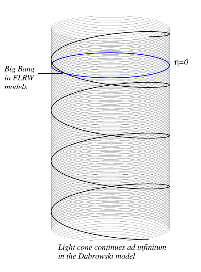
Figure 5.1: Lookback time and the past null cone on the Einstein cylinder. This shows the null structure for any model conformal to the Einstein static spacetime, including the Da̧browski and FLRW models. In FLRW models, the big bang occurs at $\eta=0$, whereas in Da̧browski models, the spacetime extends to $\eta=-\infty$.

where $\chi$ is shown as a circle ($0\leq\chi\leq 2\pi\equiv 0$), the null rays just circle around the cylinder indefinitely into the past, going round infinitely many times regardless of the initial $\eta_{0}$ (or $t_{0}$). Thus, the whole of the big-bang surface is contained within the causal past of every point of both spacetimes, and there is no horizon problem for the Da̧browski models.

We can see this in another way if we calculate the lookback time in our models (ie, the time, $t$, at which a galaxy at some position $\chi$ emits the light that the observer sees now at time $T$), which we can do using (5.12) (or directly from the metric (4.9) – see 4.28). From (5.12) and the equations for null geodesics in conformal time, $\eta=\eta_{0}(T)-\chi$ (with $\eta_{0}(T)$ given by the inverse of (5.12)) we get

$$t(\chi)=\frac{bT}{(aT+b)\exp{(b\chi/\sqrt{\Delta})}-aT}.$$ (5.14)

Note that this function is continuous through $\chi=\pi$. Again, $t\rightarrow 0$ if and only if $\chi\rightarrow\infty$. We can visualise this using the ‘Da̧browski cylinder’ of figure 5.2

Figure 5.2: As in figure 5.1, but now using the actual Da̧browski model time coordinate, $t$.

(like the Einstein cylinder but with $t$ instead of $\eta$ as the time coordinate). The null rays still asymptote to the big-bang surface, but this diagram reflects the way that in reality the spatial sections shrink as time decreases to zero: as the sections shrink (going back in time) light rays can travel all the way round the universe in a shorter and shorter time, and if the spatial sections shrink sufficiently slowly as we move back towards the big bang this travel time can approach zero without the light ray hitting the big-bang surface.

This is all in sharp contrast to FLRW universes and de Sitter space, which are conformal only to parts of the Einstein cylinder (they are bounded below at $\eta=0$): at early times the particle horizon is finite and contains only a small part of the big-bang surface, so that widely separated points can share no common influences. See figures 17 and 21 in Hawking and Ellis (1973).

The existence of a horizon is directly related to the rate at which the (FLRW or Stephani) scale factor grows for small $t$. If $R\sim t^{\alpha}$ at early times, then conformal time goes as

$$\eta\sim\int\frac{dt}{R(t)}\sim\frac{1}{1-\alpha}t^{1-\alpha}\hskip 14.22636pt\hbox{ (or $\log t$ for $\alpha=1$).}$$

So, when $\alpha<1$ (as it is for dust FLRW models) $\eta=0$ at $t=0$, the spacetime is conformal to only part of the Einstein cylinder and a horizon exists. Otherwise, as $t\rightarrow 0$ $\eta\rightarrow-\infty$ and the horizon is absent.

Other methods which lead to the solution of the horizon problem include using the LTB models; Célérier and Schneider (1998). See also Rindler (1956) who first reported the horizon problem.

5.1.1 Matter Content and Energy Conditions.

The Stephani models do not have an equation of state in the strict sense, with the relationship between pressure and energy density being position dependent. Along each flow line, however, there is a relation of the form $p=p(\mu)$ – see Krasinski (1983). The particular models we are using have an equation of state at the centre of symmetry (or everywhere in the homogeneous limit $a\rightarrow 0$) of the (exotic) form $p=-\frac{1}{3}\mu$. The matter content of these models with regard to the natural (comoving) velocity field is a perfect fluid with energy density

$$\frac{8\pi G}{c^{2}}\mu=\frac{3}{R(t)^{2}},$$ (5.15)

and pressure given by

$$p = \mu c^{2}\left(\frac{2}{3}\frac{V(r,t)}{1+\frac{1}{4}\Delta r^{2}}-1\right)$$ (5.16)

$$= -\frac{1}{3}\mu c^{2}\left(1+\frac{8aR}{c\Delta}\sin^{2}\frac{\chi}{2}\right),$$ (5.17)

$$= -\frac{1}{3}\mu c^{2}\left(1+\sqrt{\frac{24}{\pi G\mu}}\frac{a}{\Delta}\sin^{2}\frac{\chi}{2}\right),$$ (5.18)

where (5.15) has been used to express the $t$-dependence of pressure (which arises through the appearance of $R(t)$ in $V(r,t)$ – see (4.2) and (5.4)) in terms of the density. In other words, we have an ‘equation of state’ of the form

$$p=-\frac{1}{3}\mu c^{2}+\epsilon(\chi)\mu^{1/2}.$$ (5.19)

The appearance of $-\frac{1}{3}\mu$ as the dominant contribution to the equation of state immediately suggests a quintessential or scalar field model (see Frampton 1999; Liddle 1999; Coble, Dodelson and Frieman 1997; Liddle and Scherrer 1998), although it has been shown (Vilenkin 1981; Da̧browski and Stelmach 1989) that cosmic strings also give rise to this EOS. The interpretation of the Stephani matter content as a perfect fluid is by no means required; other interpretations, such as a scalar field, are equally valid, and the fact that there is no true EOS might even suggest a two-component interpretation. It is certain from chapter 3 that they will admit a thermodynamic scheme. We will discuss this in detail in a future paper. For the moment, however, this is as far as we will go to provide a physical motivation for the matter in the Da̧browski models: in this paper we are only interested in the observational consequences of the geometry; although when we impose the energy conditions below we show that the matter is certainly not obviously unphysical.

We note that the Bianchi identities lead to the following conservation equations (Ellis 1998; Wainwright and Ellis 1997)

$$\widetilde{\nabla}_{a}\epsilon=-\dot{u}_{a}(\epsilon+{\textstyle\frac{2}{3}})$$

$$\dot{\mu}=-3H(\epsilon+{\textstyle\frac{2}{3}})\mu$$

the second of which is exactly the form of the energy conservation equation for FLRW models with a ‘$\gamma$’ equation of state – note also that it shows that $\dot{\mu}$ is not homogeneous.

We can see that there are singularities of density and pressure as $R(t)\rightarrow 0$ (ie, at $t=0,-b/a$), which correspond to the big bang and crunch for these models (the metric becomes singular at these points too) – see Da̧browski (1993). We can also have a finite-density singularity, where only the pressure becomes singular. This happens when $r\rightarrow 2/\sqrt{-\Delta}$. Such infinite pressure is clearly not physical, so we can reject models with $\Delta<0$. For models with $\Delta=0$, it is difficult to compare them directly with $\Delta>0$ models due to the different geometries of the spatial sections, so we will not consider them in this thesis, and we are left with $\Delta>0$, ie, $b<1$ – see (5.5). As we explained in §4.1 the natural assumption that $R(t)>0$ after the big bang ensures that $b\geq 0$ ($\Delta\leq 1$).

Having calculated the pressure and density of the fluid we can now investigate its physical viability through the energy conditions. It is more convenient to use the original stereographic coordinates for this (ie, expression (5.16) for the pressure), since we wish to consider all values of $\Delta$, until we find reasons to the contrary. The weak energy condition states that $\mu\geq 0$ and $p+\mu c^{2}\geq 0$, whereas the strong energy condition is equivalent to $3p+\mu c^{2}\geq 0$ (see, for example, Wald 1984 for a discussion). The weak energy condition does not constrain our models at all: it implies that $V\geq 0$, but this is always true since $V\rightarrow 0$ only at spatial (and temporal) infinity (even though the coordinates themselves may be finite). The strong energy condition, however, implies that $\kappa(t)\geq\Delta$ for all $t$. From (5.4) we can see that this is equivalent to $a\leq 0$ (since $R>0$), so the models must have a big crunch ($R(t)$ is an ‘upside-down’ quadratic).

The dominant energy condition is more interesting. It states that $|p|\leq\mu c^{2}$, from which (5.15) and (5.18) immediately give

$$0\leq\frac{1}{3}\frac{V(r,t)}{1+\frac{1}{4}\Delta r^{2}}\leq 1.$$

The left inequality requires only that $\Delta\geq 0$, which rules out infinities in the pressure (finite-density singularities). The inequality on the right says that for all $t$ and $r$

$$(\kappa(t)-3\Delta)r^{2}\leq 8$$ (5.20)

must hold. This condition is always true for $a\geq 0$ (see (5.4)), as long as $\Delta\geq 0$. When $a<0$, $r$ is unbounded (for $\Delta\geq 0$, because $\kappa$ is then positive – see (4.2)), so the left hand side of (5.20) must always be negative, ie, $\kappa(t)\leq 3\Delta$. It is easy to show that $R(t)/c\leq-b^{2}/4a$, so, from (5.4),

$$\kappa(t)\leq 1.$$

Then $\kappa\leq 3\Delta$ for all $t$ provided

$$b\leq\sqrt{\frac{2}{3}}\approx 0.82.$$ (5.21)

For $b$ larger than this the dominant energy condition will be broken at some time, in regions of the universe at large $r$. We will not consider further the intricacies of this. A glance at the exclusion diagrams, figures 5.12 and 5.13, shows that (5.21) does not eliminate a significant area of the allowed region. In light of this we will, for the moment, overlook (5.21) and investigate the properties of all models with $0<b<1$.

To summarise: we have used basic physical requirements, such as the occurrence of a big bang and the avoidance of pressure singularities, and energy conditions to restrict the ranges that the two parameters $a$ and $b$ (or $\Delta$) can take. The results are:

$$a\leq 0,\phantom{h}0<b<1\phantom{h}\hbox{(ie, $0<\Delta<1$)}$$ (5.22)

(we reject $b=1$ for simplicity, as explained above, and we refrain from invoking (5.21) until §5.5). Of course, we are not forced to accept the energy conditions. Although they seem physically very reasonable conditions to impose on any form of matter there are many examples of cosmological models based on matter that does not satisfy them (quantum fields, for example, can exhibit negative energy density). However, we will assume their validity and in most of what follows we only investigate the properties of the models satisfying (5.22).

5.2 Constraining the Model Parameters Using Observations.

So far we have considered only the ‘global’ physical properties of Da̧browski models, but to really assess their potential viability as cosmological models it is necessary to confront them with observations. In this section we derive the distance-redshift relations that form the basis of the classical cosmological tests and compare them with available observational constraints to see whether any regions of parameter space are capable of providing a fit. We will impose constraints on the value of $H_{0}$, age, size (the meaning of which will be explained below) and the anisotropy of the microwave background, leaving the wealth of data available from galaxy surveys and high-redshift supernovae for consideration in a future paper; the complexities involved in interpreting such data and applying it to idealised cosmological models require separate treatment.

To recap from chapter 4, when the change of coordinates is made to an arbitrary location, we have the metric (4.23) with $W$ restricted to

$$W\rightarrow W(\chi,\psi,\vartheta;t)=1-\frac{2aR(t)}{c\Delta}(1-\cos\psi\cos\chi+\sin\psi\sin\chi\cos\vartheta).$$ (5.23)

Using the expression for the lookback time (5.14) and the expression for the redshift (4.30 and our simplified expression for $W$ (5.11) we find

$$1+z(\psi,\chi,\theta) \!\!\!\!= \!\!\!\!\frac{R_{0}}{W_{0}}\frac{W(\psi,\chi,\theta;t)}{R(t)}$$ (5.24)

$$\!\!\!\!= \!\!\!\!\frac{R_{0}}{W_{0}}\left\{\frac{1}{R(t)}-\frac{2a}{c\Delta}\left(1-\cos\psi\cos\chi\right)-\frac{2a}{c\Delta}\sin\psi\sin\chi\cos\vartheta\right\};$$

where $R_{0}=R(T)$, $W_{0}=W(\psi,T)$, showing that, for objects at any fixed $\chi$, the inhomogeneity of universe manifests itself in the redshift as a pure dipole in angle around the sky ($\cos\vartheta$ term). This will be important in §5.2.4.

For metrics with spherical symmetry about the observer the angular size (and area) distance is given directly from the coefficient in front of the angular part of the metric, because symmetry ensures that for radial rays $\vartheta$ and $\varphi$ are constant along the trajectory. For our models we do not have spherical symmetry about every observer, but the metric is everywhere conformal to a spherically symmetric metric, as can be seen from (4.9). Since null rays are not affected by the conformal factor they also remain at fixed $\vartheta$ and $\varphi$, so we can again obtain the angular size distance, $r_{A}$, from the coefficient of the angular part of the metric:

$$r_{A}(\psi,\chi,\vartheta)=\frac{R(t)}{\sqrt{\Delta}W(\psi,\chi,\vartheta;t)}|\sin\chi|$$ (5.25)

(again, $\chi$ and $t$ are related by (5.14)). We can find, for the first time, the exact angular size distance relation parametrically by combining equations (4.39) and (4.29), which bypasses the rather cumbersome method of Kristian and Sachs (1966). This is valid for any null-connected points in the spacetime.

Luminosity distance, $r_{L}$, is related to $r_{A}$ by the reciprocity theorem:

$$r_{L}=(1+z)^{2}r_{A},$$ (5.26)

see MacCallum and Ellis (1970) and Ellis (1998). This then allows the magnitude-redshift relation to be determined in the usual way: the apparent magnitude $m$ of an object of absolute magnitude $M$ is given in terms of the luminosity distance by

$$m-M-25=5\log_{10}r_{L}.$$ (5.27)

The task now is to limit $a$, $b$, and $T$ using present observational constraints. A full discussion of each constraint is made in the following sections, and they are followed by exclusion diagrams showing the regions of parameter space for which $a$ and $b$ give a plausible cosmological model for all observer locations in these models.

5.2.1 Hubble’s Constant.

The expansion rate of the universe has been measured with reasonable accuracy. Hubble’s constant is believed to lie in the range $50\mathrel{\vbox{\hbox{\tiny\ooalign{\raise 3.25pt\hbox{$<$}\crcr$\sim$}}}}H_{0}\mathrel{\vbox{\hbox{\tiny\ooalign{\raise 3.25pt\hbox{$<$}\crcr$\sim$}}}}80$ km s^-1 Mpc^-1, and we will use these limits to constrain the Da̧browski models. The Hubble parameter for these models is independent of position (4.5):

$$H\!\!\mathrel{\vbox{\hbox{ \ooalign{\raise 4.75pt\hbox{${\textsf{\tiny{\,def}}}$}\crcr$=$}}}}\frac{\theta}{3}=\frac{{R}(t)_{,t}}{R(t)}\phantom{\ }\Longrightarrow\phantom{\ }H_{0}=\frac{{R}_{,t}(T)}{R(T)}.$$ (5.28)

We can use this to place constraints on the time at which observations can be made at any position: for our models $H$ decreases monotonically, so it will only lie in the observed range of $H_{0}$ for some range of $T$. For any observer with coordinate age $T$, we require

$$50\mathrel{\vbox{\hbox{\tiny\ooalign{\raise 3.25pt\hbox{$<$}\crcr$\sim$}}}}\frac{2aT+b}{aT^{2}+bT}\mathrel{\vbox{\hbox{\tiny\ooalign{\raise 3.25pt\hbox{$<$}\crcr$\sim$}}}}80.$$ (5.29)

Usually, for simplicity, we will choose a specific value for $H_{0}$ (almost invariably that which produces the ‘worst case’). Then we can solve (5.28) for $T$.

However, when $H_{0}$ is actually measured, it is not necessarily equal to the expansion rate. What is measured in practice is the lowest order term in the magnitude-redshift relation, which gives the measured Hubble’s constant, $H^{m}_{0}$:

$$H^{m}_{0}=\left.\frac{k^{a}k^{b}\nabla_{a}u_{b}}{(u_{c}k^{c})^{2}}\right|_{0}$$ (5.30)

(where $k^{a}$ denotes the wave-vector of the incoming photons); see MacCallum and Ellis (1970). Equivalently, we can consider the gradient of the redshift-area distance curve at the observer (cf. Humphreys et al. 1997). The covariant derivative of the velocity field that appears in (5.30) can be decomposed in terms of the expansion, acceleration, shear and rotation of the flow. In the case of the Stephani models these last two are zero, so

$$\nabla_{b}u_{a}=Hh_{ab}-\dot{u}_{a}u_{b}.$$ (5.31)

Therefore the measurement of $H^{m}_{0}$ depends upon the acceleration of the observer. If we measure the magnitude-redshift relation for objects in some direction, then, comparing equation (5.30) with the expansion given by (5.28), we find

$$H^{m}_{0}(\theta)=H_{0}-\frac{\dot{u}}{c}\cos\theta,$$ (5.32)

where $\dot{u}$ is the acceleration scalar and $\theta$ is the angle between the acceleration vector and the direction of observation (which is opposite to the direction in which the photons are travelling). Since the acceleration is non-zero in the Stephani models there will be a dipole moment in $H^{m}_{0}$. The size of this in the Da̧browski models is given directly from (4.12). If this is large in any model we can probably reject that model because a large dipole moment in $H_{0}$ is not observed. However, nearby it is difficult to measure $H_{0}$ accurately due to peculiar motions and the discreteness of galaxies. There is a dipole moment in observations of more distant objects, which is assumed to be due to the fact that the Local Group is falling into the potential well produced by Virgo and the Great Attractor. The question is: what upper bound can be placed on the acceleration by observations? This issue will be discussed in §5.2.5. For now we simply use (5.29) to constrain the epoch of observation, $T$.

Hubble Normalised Scalars

If we wish to define, in analogy with FLRW models, Hubble normalised scalars, then we can do so as follows. We define

$$\Omega \!\!\!\!= \!\!\!\!{\frac{24\pi G\mu}{\theta^{2}}}=(2at+b)^{-2},$$ (5.33)

$$\Omega_{p} \!\!\!\!= \!\!\!\!{\frac{24\pi Gp}{c^{2}\theta^{2}}}=-{\frac{1}{3}}\Omega\left(1+{\frac{8aR}{c\Delta}}\sin^{2}{\frac{\chi}{2}}\right).$$ (5.34)

We can get a fairly good idea how these models behave, in comparison with what is know from local observations. We recall that

$$0.3\mathrel{\vbox{\hbox{\tiny\ooalign{\raise 3.25pt\hbox{$<$}\crcr$\sim$}}}}\Omega_{0}\mathrel{\vbox{\hbox{\tiny\ooalign{\raise 3.25pt\hbox{$<$}\crcr$\sim$}}}}1,~{}~{}~{}0\mathrel{\vbox{\hbox{\tiny\ooalign{\raise 3.25pt\hbox{$<$}\crcr$\sim$}}}}\Omega_{\Lambda_{0}}\mathrel{\vbox{\hbox{\tiny\ooalign{\raise 3.25pt\hbox{$<$}\crcr$\sim$}}}}1$$ (5.35)

for the present-day values of the density parameter and cosmological constant. For the Da̧browski models, we note that in the limit $t\rightarrow 0$ we have

$$\Omega={\frac{1}{b^{2}}},~{}~{}~{}\Omega_{,t}=-{\frac{4a}{b^{3}}}.$$ (5.36)

We know that $b$ is positive in order that the scale factor is positive, which implies that $\Omega_{,t}$ is negative at the big bang only if $a>0$. However we also see that as $t\rightarrow 0$, then $\Omega$ approaches some value larger than $1$ if $b<1$, as required by neglecting models with a finite density singularity. This means that if we desire $\Omega\mathrel{\vbox{\hbox{\tiny\ooalign{\raise 3.25pt\hbox{$<$}\crcr$\sim$}}}}1$ today, then we force $a>0$, in contradiction with the strong and dominant energy conditions (but not the weak one).

As far as the quantity ‘$\Omega_{p}$’ is concerned, we may ‘equate’ it with the cosmological constant term of the standard model. If we consider the expression for $q$, the deceleration parameter, given by equation (2.154) (which is essentially the Raychaudhuri equation) then the standard model has

$$q={\textstyle\frac{1}{2}}\Omega-\Omega_{\Lambda}$$ (5.37)

while for the Da̧browski models we may write

$$q\approx{\textstyle\frac{1}{2}}\Omega+{\textstyle\frac{1}{2}}\Omega_{p}$$ (5.38)

neglecting the acceleration terms (which are zero at the center). We may therefore identify

$$\Omega_{p}\simeq-2\Omega_{\Lambda}.$$ (5.39)

Thus we may equate a positive cosmological constant with a negative pressure parameter. If we require this for all locations today (which means that $R$ is quite small) then the sign of $a$ doesn’t matter: however, there will be a time (at $t=-b/2a+\sqrt{3b^{2}-1}/2\sqrt{2}a$) when the sign of $\Omega_{p}$ changes if $a$ is negative. Of course we should take into account acceleration in the ‘definition’ of $\Omega_{\Lambda}$, but this is only a qualitative discussion.

What is interesting is that while the strong and dominant energy conditions favour $a<0$, this seems to be ruled out by current measurements of the matter density of the universe.

This may give cause for concern for these models, but it does not really concern us here. We will carry on with the analysis of models with $a<0$ throught this thesis, because we are more concerned with the Copernican principle in a non-standard cosmology, rather than finding the ‘best-fit’ IRF model (although, it will be shown in §5.4 that SNIa data favour $a>0$ too). This will be discussed later.

5.2.2 The Age of the Universe.

The original inspiration for Da̧browski and Hendry (1998) to study Stephani models was the potential resolution of the age problem that they provided, which at that time seemed to be virtually insurmountable within the framework of FLRW models (even when a non-zero cosmological constant was invoked): the high measured value of $H_{0}$ suggested an age, $\tau_{0}$, of at most about $11$ Gyr for a FLRW cosmology, whereas globular cluster ages were thought to be at least $12$-$13$ Gyr (Hendry and Tayler, 1996; Chaboyer et al. 1998). Da̧browski and Hendry (1998) and Paper I showed that, for the particular Stephani models they considered, this apparent paradox disappears: the Da̧browski models have ages that are consistently 1-4 Gyr older than their FLRW counterparts (for an observer at the centre of symmetry, at least). However, the age problem has recently been alleviated by a recalibration of the RR Lyrae distance scale and globular cluster ages in the light of Hipparcos (Chaboyer et al. 1997), which has reduced the globular cluster ages considerably, to $\sim 10$ Gyr. The fit is still marginal, but the new ages are generally accepted as they allow a flat FLRW model to fit the observations provided that $H_{0}\mathrel{\vbox{\hbox{\tiny\ooalign{\raise 3.25pt\hbox{$<$}\crcr$\sim$}}}}67$ km s^-1 Mpc^-1.

We certainly require, then, that at the epoch of observation our models are older than $10$ Gyr. However, we will also consider the stronger constraint $\tau_{0}>12$ Gyr, partly to be conservative, but also because the diagrams for the $12$ Gyr constraint are often clearer. Since it was shown in Paper I that best fit Da̧browski models are significantly older than their FLRW counterparts, we do not expect problems from this constraint. There is a surprise in store, though, when we consider non-central observers, and age will turn out to be the dominant constraint on these models.

The age of the universe according to an observer at position $\psi$ and at coordinate time $T$ is simply the proper time elapsed from the big bang ($t=0$):

$$\tau_{0} \!\!\!\!= \!\!\!\!\int_{0}^{T}\frac{dt}{W(\psi,t)}$$ (5.40)

$$\!\!\!\!= \!\!\!\!\frac{\Delta}{4|a|\sin\frac{\psi}{2}\sqrt{1-b^{2}\cos^{2}\frac{\psi}{2}}}\ln\left\{\frac{\Delta-\Sigma_{+}}{\Delta-\Sigma_{-}}\right\}$$

where

$$\Sigma_{\pm}=\left(b\sin\frac{\psi}{2}\pm\sqrt{1-b^{2}\cos^{2}\frac{\psi}{2}}\right)2aT\sin\frac{\psi}{2}$$

(for $a\neq 0$ and $\psi\neq 0$: otherwise $W\equiv 1$ and $\tau_{0}=T$), where we take the value of $T$ given by the solution of equation (5.28) as our constraint on the coordinate time for any specific $H_{0}$. In figure 5.3

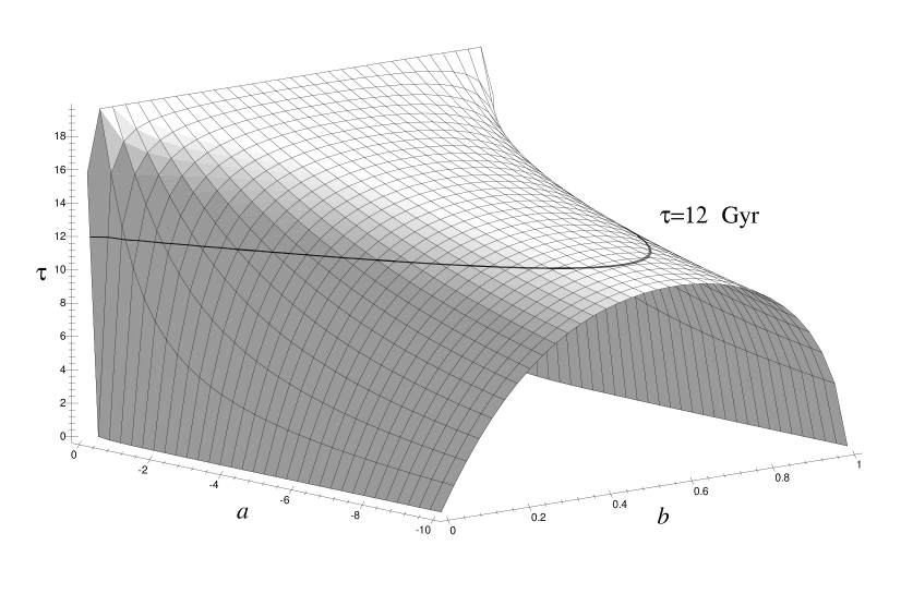
Figure 5.3: Surface plot of the proper age of the universe for $H_{0}=50$ km s^-1 Mpc^-1 with the observer at $\psi=\pi$.

we show proper age for observers at $\psi=\pi$ with $H_{0}=50$ km s^-1 Mpc^-1 (which shows the behaviour of the age function most effectively) as $a$ and $b$ vary. The contour at $\tau_{0}=12$ Gyr is also drawn. As can be seen, below this curve the values of $a$ and $b$ can be rejected – the proper age is too low.

In figure 5.4

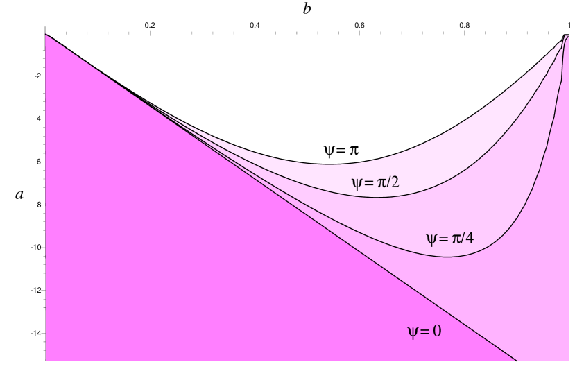
Figure 5.4: $\tau_{0}=12$ Gyr exclusion plot for different observer positions, for $H_{0}=60$ km s^-1 Mpc^-1. In the shaded areas the models are not old enough. $\psi=\pi$ is clearly the most restrictive case.

the $\tau_{0}=12$ Gyr contours of the proper age function are plotted for $H_{0}=60$ km s^-1 Mpc^-1 and for several observer positions, $\psi$, showing how the age of an observer varies with $\psi$ for different parameters $a$ and $b$. The shaded regions contain models that are less than $12$ Gyr old for at least one of the observer positions. This demonstrates that the proper age of an observer is smallest at the antipodal centre of symmetry, $\psi=\pi$, so the contour at $\tau_{0}=12$ Gyr in figure 5.3 marks the limit of viable models for this age constraint. Consequently, we will always use proper age at $\psi=\pi$ to constrain the model parameters. We could weaken this constraint by requiring only that most observers are old enough, which would allow us to consider instead the age of observers at $\psi\leq\pi/2$ while still satisfying the Copernican principle (half of the observers would lie in this region). For simplicity, though, we will not do this here.

Finally, in figure 5.5

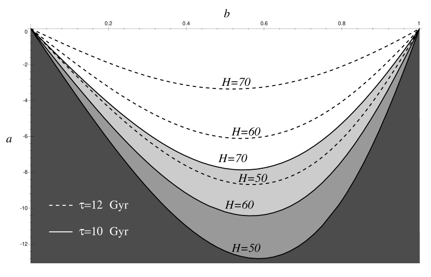
Figure 5.5: The age exclusion diagram for various $H_{0}$ and proper age $\tau=10$ Gyr. The shaded region represents the prohibited area. Also shown as dashed lines are the age limits for $\tau=12$ Gyr. (Note that the region excluded for $H_{0}=70$ km s^-1 Mpc^-1 contains the excluded regions for lower $H_{0}$ – the progressively darker shading indicates this.)

we show the age exclusion plot for the models (based on proper age at $\psi=\pi$). We use three values of $H_{0}$: $50$, $60$, and $70$ km s^-1 Mpc^-1, and a proper age of $10$ Gyr (although the limits for $12$ Gyr are also indicated). The shaded regions are excluded. It can be seen that unless we require the universe to be particularly old or the expansion rate high there is still a significant region of parameter space that cannot be excluded on the basis of age.

It should be noted here that these plots are meaningless for $b=1$, because then $\Delta=0$ and the model is conformal to an FLRW model with flat spatial sections, for which $\chi$ is not a good coordinate – as can easily be seen from (4.8).

5.2.3 Size and the Distance-Redshift Relation.

When the spatial sections of a cosmological model are 3-spheres it may be possible for light rays to circle the entire universe, perhaps a large number of times. This is indeed the case for the models we are considering here. What will the signature of this be in the various distance-redshift relations? For the Da̧browski models this is a particularly easy question to answer because the fact that they are manifestly conformal to FLRW models allows us to determine the paths of light rays directly from the null geodesics of the underlying FLRW space. From this it is clear that light rays from a point directly opposite the observer (ie, from the antipode, $\chi=\pi$) will spread out around the universe isotropically from the antipode until they pass the ‘equator’ ($\chi=\pi/2$), where they will begin to converge and be focused onto the observer. As a result, a point source positioned exactly at the antipode will fill the entire sky when seen by the observer, so that its angular size distance, $r_{A}=$ (physical length/apparent diameter), is zero. Similarly, the refocusing of light onto a point produces an infinite flux at the observer, and therefore the luminosity distance, $r_{L}$, is also zero ($m\sim\log_{10}r_{L}=-\infty$). Precisely the same argument applies to light that leaves the observer’s position, travels through the antipode (where it will be focused to a point), and returns to the observer (being focused a second time). In fact, it is obvious that whenever the light rays travel through a parameter distance $\chi$ that is an exact multiple of $\pi$, $r_{A}=r_{L}=0$: this is reflected by the factor of $\sin\chi$ in (4.39).

This effect can be seen clearly in figures 5.6-5.8, where we show the two principle measures of distance as they vary both with coordinate distance $\chi$ and redshift. Viewed as a function of $\chi$, in figure 5.6,

Figure 5.6: Area distance from the centre as a function of $\chi$ for two values of $b$. $T=15$ Gyr, $a=-1$.

the zeros of the angular diameter distance clearly occur at multiples of $\pi$ for all model parameters. Looked at in terms of redshift, though (figure 5.7),

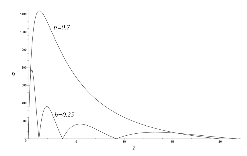
Figure 5.7: Area distance from the centre as a function of redshift for the same parameters as figure 5.6. For small $b$ the angular size distance oscillates far too rapidly.

it is clear that for small $b$ the zeros are much closer together than for larger $b$, with the first zero occurring at $z\approx 1$ for $b=0.25$. Figure 5.8

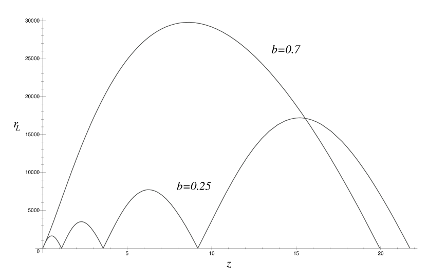
Figure 5.8: Luminosity distance from the centre as a function of redshift for the same parameters as figures 5.6 and 5.7.

shows the luminosity distance-redshift relation, for comparison. These effects are not as unusual as they look, and can be found also in FLRW geometries for models with positive $\Lambda$ – see §4.6.1 in Ellis (1998) and references therein. It is noteworthy that a blackbody situated at the opposite pole to the observer would look exactly like the CMB if it was at the right redshift. For example, a star of surface temperature 3000K at a redshift $z=1000$ would have an apparent temperature of 3K, and would cover the whole sky.

Can we rule out such apparently aberrant behaviour? Theories of structure formation are fairly well developed (see Bertschinger et al. 1997 for a thorough discussion and references), and the evolution of galaxies and the star formation rate (SFR), while not accurately known, are at least qualitatively understood. In particular, the SFR, which is very important for determining the luminosity of distant, young galaxies, is believed to fall off beyond $z\sim 3$ (see, for example, Loeb, 1999). As a result, one could argue that there will be relatively few bright objects beyond some redshift $z_{SF}$ that corresponds to the epoch at which galaxies ‘turned on’ and the SFR began to increase significantly. This would mean that the zeros in the distance-redshift relations would be essentially unobservable if they occurred at redshifts larger than $z_{SF}$ because there would be no luminous objects to be seen magnified in the sky, whereas if the zeros occurred at lower redshifts than $z_{SF}$ one could reasonably argue that there ought to be some signature of this in the observations. Since galaxies have only been observed (in the Hubble Deep Field, for example) with redshifts up to $z\sim 5$ we take $z_{SF}=5$ (although the constraints imposed by larger $z_{SF}$ can easily be inferred from the exclusion diagram, figure 5.9). If these arguments are not completely convincing, then, at a simpler level, the fact that the observed magnitude-redshift relation is known accurately out to $z\sim 1$ from type Ia supernovae (Perlmutter 1999), and is certainly not dipping down, allows us to say that there is no zero of luminosity distance below $z\sim 2$, say. We therefore also consider the constraint that results from requiring that there are no zeros below $z=2$.

We wish, then, to constrain the parameters of our models by rejecting any models for which the first zero in the distance-redshift relations occurs at $z\leq z_{\pi}$, where $z_{\pi}=2$ or $z_{\pi}=z_{SF}=5$. Using (4.29), this means

$$1+z(\chi=\pi)=\frac{R_{0}}{W_{0}}\frac{W(\psi,\pi,t_{\pi})}{R(t_{\pi})}>1+z_{\pi},$$ (5.41)

where $R_{0}=R(T)$, $W_{0}=W(\psi,T)$ (giving the conformal factor at the observer) and $t_{\pi}$ denotes the lookback time (5.14) at $\chi=\pi$. Again we determine the epoch of observation (ie, the observer’s coordinate time $T$) using (5.28). The solution of (5.41) for $a$ and $b$ is shown in figure 5.9 as an exclusion diagram.

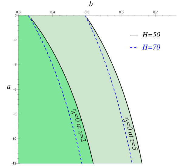
Figure 5.9: Exclusion plot obtained by requiring that the first zeros of $r_{A}(z)$ occur at $z>z_{\pi}$, for $z_{\pi}=2$ and $z_{\pi}=5$. The shaded regions are excluded. Curves are given for $H_{0}=50$ and $H_{0}=70$ km s^-1 Mpc^-1.

The effect of this constraint is to rule out small values of $b$, for any $a$. This is a reflection of the fact that, loosely speaking, $b$ measures the ‘size’ of the universe: for small times the scale factor goes as $bt$, so that when $b$ is small the spatial sections are small, light rays don’t take long to travel from antipode to observer, the scale factor changes relatively little during this time and the redshift of the antipode (which is dominated by $R_{0}/R(t_{\pi})$ as in FLRW models) is small.

As a coda to this section we consider the effect of demanding that the first zero of $r_{A}$ is effectively unobservable as a result of being ‘hidden’ behind the CMB. Figure 5.10

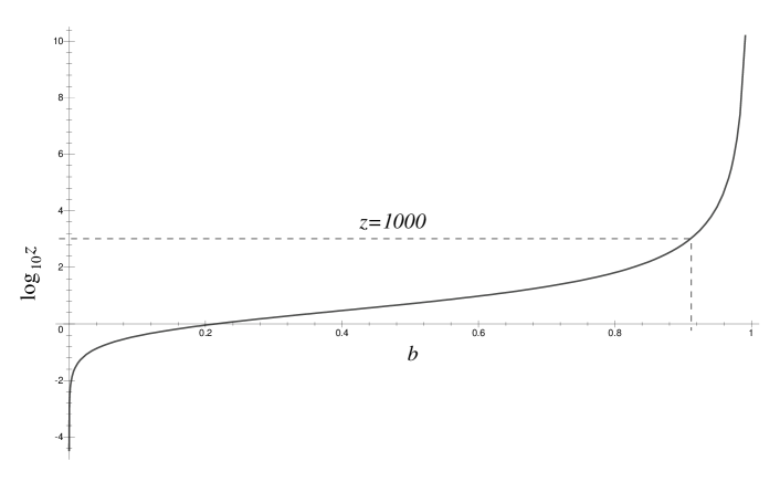
Figure 5.10: Logarithmic plot of the redshift at which the first zero of $r_{A}$ occurs as a function of $b$ for $H_{0}=50$ km s^-1 Mpc^-1 and $a=-1$. For the first zero to occur at $z>1000$, so that recombination occurs ‘nearer to us’ than the antipode – ie, at $\chi<\pi$ – requires $b\approx 1$.

shows how the redshift of the first zero of $r_{A}(z)$ varies with $b$. If, instead of choosing $z_{\pi}=z_{SF}$ as our primary constraint, we want the first zero of $r_{A}(z)$ to happen at a redshift large enough for the universe to be opaque (ie, before decoupling), then figure 5.10 shows that $b$ must be quite close to unity. This figure also allows the extent to which values of $b$ are excluded for any $z_{\pi}$ to be estimated.

5.2.4 The Microwave Background Anisotropy.

The CMB is observed today to be a blackbody at a temperature of $T_{0}=2.734\pm 0.01$K, with a dipole moment of $T_{1}=3.343\pm 0.016\times 10^{-3}$K and quadrupole moment as big as $T_{2}=2.8\times 10^{-5}$K (see Partridge 1997 for details and references). It was emitted at a time when the radiation was no longer hot enough to keep hydrogen ionised, causing it to decouple from matter, which happens at $T_{\mathrm{dec}}\sim 3000$K. Idealised cosmological models do not have realistic thermodynamics (that is, they do not, in general, describe the thermodynamic evolution of the gas and radiation mixture that fills the real universe). In FLRW models the epoch at which decoupling occurs is simply defined to be that corresponding to the redshift necessary to shift the temperature at decoupling to the observed mean temperature of the CMB, $T_{0}$. From the redshift relation applied to the temperature of a blackbody ($T$ will be used to denote temperature in this section),

$$T_{\mathrm{obs}}=\frac{T_{\mathrm{dec}}}{1+z},$$ (5.42)

we infer that the CMB is formed at a redshift $z\approx 1000$. This definition is fine for homogeneous models, leading to a consistent definition of the time of decoupling for every observer at the same cosmic time, but raises an interesting point for the inhomogeneous Da̧browski models, because the redshift depends on both the observer’s position, $\psi$, and the angle around the sky, $\theta$. If we simply define the redshift of the CMB at any point to satisfy (5.42) with $T_{\mathrm{obs}}=T_{0}$ then, by definition, we obtain a perfectly isotropic CMB for that observer, but we must choose a different emitting surface for each different observer. Such an observer-based definition of the CMB surface is clearly unsatisfactory. Instead we propose several alternative ways to define what is meant by the CMB surface (it is important in these definitions to distinguish between the dominant strange matter that is responsible for the geometry of the Da̧browski models – see §5.1.1 – and the putative ‘real’ gas that decouples):

1. On a surface of constant cosmic time, $t=t_{\scriptscriptstyle{CMB}}$ – since the Da̧browski models possess a cosmic time coordinate with respect to which only the pressure is inhomogeneous this is a natural extension of the FLRW definition;

2. In general inhomogeneous models we could choose hypersurfaces of constant density, which at least has some physical basis – for the Da̧browski models this is equivalent to 1. because the density is homogeneous on cosmic time surfaces;

3. On surfaces such that $p/\rho=$constant (which gives constant temperature for an ideal gas) – for our models this would mean that decoupling occurs at different times at different places in the universe (probably a good thing in an inhomogeneous universe); however, the Da̧browski matter is not an ideal gas so the validity of this definition for these models is debatable;

4. On a surface of constant proper time (based on the assumption of some common evolution for the ideal gas component at different positions) – see equation (5.40);

5. Finally, we could avoid all consideration of the physics of decoupling and simply assume that it happens at such an early time that we can effectively define the CMB to be free-streaming radiation ‘emitted at the big bang’, as is implicitly assumed in the EGS theorem (Ehlers, Geren and Sachs 1968). This only really makes sense if there is some natural definition of the radiation field at early times. For example, if the model is homogeneous and isotropic at early times, we can define a homogeneous and isotropic radiation field. Our models have exactly this property of homogeneity at early times (as can be seen from (5.10), if $t\rightarrow 0$ then $W\rightarrow 1$).

Although 5) is interesting we will not consider it here because it does not reflect the physics of the CMB, and, on a more practical level, it prevents us from constraining the CMB anisotropy, because there isn’t one. Also, the homogeneity of Da̧browski models at early times means that for small $t$ the proper age is virtually identical to the coordinate time $t$ (equation (5.40) with $W\approx 1$). It turns out that for times of observation that reproduce the observed $H_{0}$ any reasonable definition of the CMB surface puts it at an early time, which means definition 4) is virtually identical to 1) We will therefore define the CMB according to 1) in this section.

It still remains, though, to decide exactly which surface of constant cosmic time the CMB originates from. Consider, for an observer at position $\psi$, the temperature distribution on the sky that the CMB would have if it were emitted from the surface $t=t_{\scriptscriptstyle{CMB}}$ (related by the lookback time formula (5.14) to some distance $\chi_{\scriptscriptstyle{CMB}}$):

$$T_{\mathrm{obs}}(\psi,\chi_{\scriptscriptstyle{CMB}},\theta)=\frac{T_{\mathrm{dec}}}{1+z(\psi,\chi_{\scriptscriptstyle{CMB}},\theta)}.$$ (5.43)

Equation (5.24) shows that we can write

$$1+z(\psi,\chi_{\scriptscriptstyle{CMB}},\theta)=1+z_{0}(\psi,\chi_{\scriptscriptstyle{CMB}})+z_{1}(\psi,\chi_{\scriptscriptstyle{CMB}})\cos\theta$$

where

$$1+z_{0}(\psi,\chi_{\scriptscriptstyle{CMB}}) = \frac{R_{0}}{W_{0}}\left[\frac{1}{R_{\scriptscriptstyle{CMB}}}-\frac{2a}{c\Delta}\left(1-\cos\psi\cos\chi_{\scriptscriptstyle{CMB}}\right)\right],$$

$$z_{1}(\psi,\chi_{\scriptscriptstyle{CMB}}) = -\frac{2a}{c\Delta}\frac{R_{0}}{W_{0}}\sin\psi\sin\chi_{\scriptscriptstyle{CMB}}=\frac{\dot{u}(\psi)}{c^{2}}\frac{R_{0}}{\sqrt{\Delta}W_{0}}\sin\chi_{\scriptscriptstyle{CMB}}$$ (5.44)

(using (4.12) in the last equality and assuming $a\leq 0$). The mean redshift of the CMB surface is $z_{0}$; $z_{1}$ gives rise to an anisotropy in the CMB. We can therefore define the location of the CMB surface to be the $t_{\scriptscriptstyle{CMB}}$ (or $\chi_{\scriptscriptstyle{CMB}}$) that gives a mean redshift of 1000. That is, $\chi_{\scriptscriptstyle{CMB}}$ is the solution of

$$z_{0}(\psi,\chi_{\scriptscriptstyle{CMB}})=1000$$ (5.45)

for any observer position $\psi$.

Having found $\chi_{\scriptscriptstyle{CMB}}$ we can evaluate the anisotropy in the temperature of the CMB. Since $T_{\mathrm{obs}}$ depends on the reciprocal of $1+z$ the dipole moment in $z$ will give rise to higher multipoles when expanded as a binomial series:

$$T_{\mathrm{obs}}(\theta)=\frac{T_{\mathrm{dec}}}{1+z_{0}}\left[1-\frac{z_{1}}{1+z_{0}}\cos\theta+\left(\frac{z_{1}}{1+z_{0}}\right)^{2}\cos^{2}\theta+O(\cos^{3}\theta)\right],$$ (5.46)

that is,

$$\frac{\delta T(\theta)}{T}=-\frac{z_{1}}{1+z_{0}}\cos\theta+\left(\frac{z_{1}}{1+z_{0}}\right)^{2}\cos^{2}\theta+O(\cos^{3}\theta).$$ (5.47)

The dipole moment of the CMB temperature is then (using (5.45))

$$\delta_{1}=\frac{z_{1}}{1+z_{0}}\approx 10^{-3}z_{1}.$$ (5.48)

Measurements of the CMB can now be used to constrain the model parameters. We at least require that the dipole moment should be no larger than the observed dipole anisotropy, $|\delta_{1}|<T_{1}/T_{0}\approx 10^{-3}$ (ie, $|z_{1}|<1$). If this is satisfied for any model then it is clear that the quadrupole and higher multipole moments will all be $\mathrel{\vbox{\hbox{\tiny\ooalign{\raise 3.25pt\hbox{$<$}\crcr$\sim$}}}}10^{-6}$ – certainly no larger than their observed values. In fact, such a constraint on $z_{1}$ is very weak, leaving vast tracts of parameter space entirely untouched. Moreover, there are very good reasons for believing that there is a significant contribution to the observed dipole moment from the peculiar velocity of the Local Group as a result of infall towards the Great Attractor (Lynden-Bell et al. 1988), which can be measured with moderate accuracy using galaxy surveys, and seems to be consistent with the motion of the Local Group with respect to the CMB (Schmoldt et al. 1999). In an inhomogeneous cosmological model, though, one expects local anisotropies that could be interpreted as bulk flows, and it is not beyond the bounds of possibility that all of the CMB dipole and the local anisotropies could be explained purely as cosmological effects in, say, a Stephani universe without any need to invoke peculiar motions and local inhomogeneities (ie, perturbations of the perfect background cosmology). Such perturbations must exist, of course, and will make some contribution to the observed anisotropies, but it has not been shown that they are the only, or even the dominant, contributions. However, we choose here to reject iconoclasm in favour of the more conservative viewpoint that most of the observed dipole is due to the peculiar motions induced by local inhomogeneities, but that there remains some leeway – up to 10% of the observed dipole – due to observational uncertainties, for there to be a purely cosmological contribution to the CMB dipole. Then the largest dipole moment that we can accept from our models is $|\delta_{1}|<10^{-4}$, or

$$|z_{1}|<0.1.$$ (5.49)

Given any model parameters and some observer position we adopt the following procedure. First we use (5.28) to determine the epoch of observation for some $H_{0}$, as usual, then we solve for $\chi_{\scriptscriptstyle{CMB}}$ using (5.45). Having found all the parameters we need to determine $z_{1}$ we simply check (5.49) to see whether the model, or at least that observer position, must be rejected. In practice we can simply solve (5.49) as an equality to obtain $a$ as a function of $b$ at the boundary of the allowed region, and this is what is shown in figure 5.11

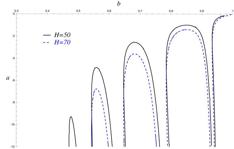
Figure 5.11: The exclusion diagram from CMB anisotropies for an observer at $\psi=\pi/2$. The curves for $H_{0}=50$, $70$ km s^-1 Mpc^-1 are shown. As $H_{0}$ increases, the ‘fingers’ move down to more negative $a$. The excluded region lies within the fingers.

(for $\psi=\pi/2$), where it can be seen that a low value of $H_{0}$ constrains our models most – in contrast to the age constraint. This is because $H_{0}$ decreases monotonically with time, so small $H_{0}$ corresponds to a later time of observation and therefore a later time for the CMB surface, which means that $W$ has evolved to become more inhomogeneous. We choose $\psi=\pi/2$ because, as is clear from (3.9) and (5.44), the anisotropy is generally worst there, so if a model is rejected at $\psi=\pi/2$ it will be unacceptable everywhere, in order to satisfy the Copernican principle. Again, therefore, for models not excluded in figure 5.11 detection of a CMB anisotropy of the magnitude that we observe would be typical, and the Copernican principle need not be abandoned for these models to be viable.

The finger-like excluded regions in figure 5.11 appear because for different model parameters $\chi_{\scriptscriptstyle{CMB}}$ takes on different values, and for some parameters this value is very close to $\pi$, so that the CMB surface is almost at the antipode of the observer. This means that the entire CMB is emitted from virtually a single point. Since redshift depends only on the relative conformal factors at emitter and observer for our conformally flat models, the CMB must be almost exactly uniform however inhomogeneous the model (ie, whatever the value of $a$).

5.2.5 The Local Dipole Anisotropy

Although we are not in a position to use real observations to constrain the dipoles that would be detected in observations of the ‘local’ universe (in galaxy surveys, for example, where $z\mathrel{\vbox{\hbox{\tiny\ooalign{\raise 3.25pt\hbox{$<$}\crcr$\sim$}}}}0.01$, or with type Ia supernova data, for which $z\mathrel{\vbox{\hbox{\tiny\ooalign{\raise 3.25pt\hbox{$<$}\crcr$\sim$}}}}1$), we can at least consider these effects qualitatively.

From (5.24) and (4.12) the redshift dipole for objects at any radius $\chi$ from an observer at $\psi$ is seen to be

$$z_{1}(\psi,\chi)=\frac{\dot{u}(\psi)}{c^{2}}\frac{R_{0}}{\sqrt{\Delta}W_{0}}\sin\chi$$

(cf. equation (5.44)). It is clear that any constraint on the anisotropy in the properties of objects at some distance from the observer will amount to a constraint on the acceleration, $\dot{u}$, of the fundamental observers, and vice versa. In the same way, constraints on the acceleration place limits on the possible dipole moment in the measured $H_{0}^{m}$ in (5.32). Defining $\delta H=\dot{u}/c$ (according to (5.32)), the dipole in redshift becomes

$$z_{1}(\psi,\chi)=\frac{R_{0}\sin\chi}{\sqrt{\Delta}W_{0}}\frac{\delta H}{c}.$$ (5.50)

If we assume that the time of observation, $T$, is fairly close to $t=0$ (as is generally the case for the values of $H_{0}$ we allow), then $W_{0}\approx 1$ and $aT\ll b$, which means that $R_{0}/c\approx bT$ and $\dot{R}_{0}/c\approx b$. Equation (5.50) then becomes, with the help of (5.28),

$$z_{1}(\psi,\chi)\approx\frac{1}{\sqrt{\Delta}}\frac{\dot{R}_{0}\sin\chi}{cH_{0}}\delta H\approx\frac{b}{\sqrt{\Delta}}\sin\chi\frac{\delta H}{H_{0}}.$$ (5.51)

Note that dependence on distance from the observer only arises through the $\sin\chi$ factor, so for observations of objects at any distance from the observer

$$|z_{1}|\mathrel{\vbox{\hbox{\tiny\ooalign{\raise 3.25pt\hbox{$<$}\crcr$\sim$}}}}\frac{b}{\sqrt{\Delta}}\frac{\delta H}{H_{0}}.$$ (5.52)

Local measurements in principle, therefore, constrain the acceleration and the anisotropy at all redshifts. For example, applying this to the CMB dipole, (5.52) shows that the constraint (5.44) imposed in §5.2.4 will always be satisfied provided that

$$\frac{\delta H}{H_{0}}\leq 0.1\frac{\sqrt{\Delta}}{b}.$$ (5.53)

To ensure that the variation in $H_{0}$ is less than 20% requires $\sqrt{\Delta}/b\leq 2$, or $b\geq 1/\sqrt{5}\approx 0.45$. For a variation of less than 10%, we must have $b\geq 1/\sqrt{2}\approx 0.71$. Since we are interested in all values of $b\mathrel{\vbox{\hbox{\tiny\ooalign{\raise 3.25pt\hbox{$>$}\crcr$\sim$}}}}0.5$ (see figure 5.12) we must be prepared to countenance variations in $H_{0}$ around the sky of up to 20% if the local anisotropy is not to impose tighter constraints on the model parameters than those already derived from the CMB. Note, though, that (5.53) is considerably stronger than is really required for most model parameters, owing to the fact that the $\sin\chi$ factor in (5.51) was neglected. This amounts to adopting as the CMB constraint the envelope of the fingers in figures 5.11, 5.12 and 5.13, which would obviously overlook large areas of parameter space that should really be allowed.

Although it would seem that the easiest way to constrain the acceleration in the Da̧browski models would be to measure the local $H_{0}$ dipole, it is not really possible to measure $\delta H/H_{0}$ accurately, because that would require accurate measurements of galaxies in different directions at very small redshifts; there are relatively few such galaxies, and those that there are possess significant random peculiar motions that make a large contribution to the errors on any estimate of $\delta H/H_{0}$. Moreover, there is known to be a dipole in observations of galaxies at somewhat larger redshifts ($z\sim 0.01$), which is usually interpreted as the effect of infall of the Local Group towards the Great Attractor (Lynden-Bell et al. 1988; Schmoldt et al. 1999). This infall manifests itself as a systematic relative motion of the Local Group with respect to distant galaxies, at a velocity $v\approx 600$ km s^-1, corresponding exactly to the Local Group motion relative to the CMB frame. In order not to conflict with these observations we at least require that at redshifts $z_{0}\approx 0.01$ the dipole moment due to the Da̧browski acceleration is no larger than the observed dipole:

$$cz_{1}\mathrel{\vbox{\hbox{\tiny\ooalign{\raise 3.25pt\hbox{$<$}\crcr$\sim$}}}}v=600\hbox{~{}km~{}s${}^{-1}$}.$$

Using (4.30) and (4.39) it is possible to rewrite (5.50) in the form

$$z_{1}(\psi,\chi)=(1+z_{0})r_{A}(\psi,\chi)\frac{\delta H}{c},$$

where we implicitly identify $z_{0}$ and $r_{A}$ as the mean redshift and angular size distance of objects at coordinate distance $\chi$. Then, since at low redshift the Hubble law is valid, $cz_{0}=v=H_{0}r_{\mathrm{prop}}$ ($r_{\mathrm{prop}}$ denotes proper distance), and $r_{A}=r_{L}=r_{\mathrm{prop}}$, we have

$$z_{1}=\frac{cz_{0}}{H_{0}}\frac{\delta H}{c}$$

That is,

$$\frac{\delta H}{H_{0}}=\frac{cz_{1}}{cz_{0}}\mathrel{\vbox{\hbox{\tiny\ooalign{\raise 3.25pt\hbox{$<$}\crcr$\sim$}}}}\frac{600\hbox{~{}km~{}s${}^{-1}$}}{0.01c}=0.2;$$ (5.54)

at most a 20% variation in $H_{0}$ around the sky, consistent with the CMB result (5.53).

Finally, we consider the magnitude-redshift relation in the low-redshift limit and apply it to type Ia supernovae (for example, to the relatively low-redshift supernovae of Hamuy et al. 1996 – although it is not unreasonable to assume that this gives at least an order-of-magnitude estimate of the size of the anisotropy for observations at higher $z$ characteristic of the supernova data of Perlmutter et al. 1999). If $z\ll 1$, then $r_{L}=cz_{0}/H_{0}$. Equations (4.41) and (5.32) give

$$m-M-25=5\log_{10}\frac{cz_{0}}{H_{0}^{m}}=5\log_{10}\frac{cz_{0}}{H_{0}}-5\log_{10}\left(1-\frac{\delta H}{H_{0}}\cos\theta\right)\approx 5\log_{10}\frac{cz_{0}}{H_{0}}+{\frac{5}{\ln 10}}\frac{\delta H}{H_{0}}\cos\theta$$

(assuming that $\delta H/H_{0}$ is small). That is,

$$\delta m={\frac{5}{\ln 10}}\frac{\delta H}{H_{0}}.$$ (5.55)

The dispersion on the magnitudes of type Ia supernovae (due to both observational errors and intrinsic dispersion) is estimated to be $\delta m\sim 0.3$ (Hamuy et al. 1996; Perlmutter et al. 1999). For the dipole resulting from the acceleration to be undetectable via type Ia supernovae we must have

$$\frac{\delta H}{H_{0}}\mathrel{\vbox{\hbox{\tiny\ooalign{\raise 3.25pt\hbox{$<$}\crcr$\sim$}}}}0.14.$$ (5.56)

This is somewhat stronger than the other local constraints derived above, and would suggest that the supernova data will indeed restrict the model parameters more than the CMB anisotropy. Comparison with (5.53) and (5.54) suggest that $b$ may only be half or a quarter as large as would be permitted by the CMB constraint (see equations (5.32) and (4.12)). However, these are only very approximate results, and require more detailed analysis. In particular, there is observed to be a dipole in the supernova data (explained in exactly the same way as the other dipoles in the conventional interpretation), and this means that the constraint (5.56) must be re-evaluated: the real constraint is likely to be somewhat weaker than (5.56).

It should be borne in mind that throughout the preceding discussion we have only considered the modulus of the dipole, not its direction. It is clear from (5.44) that the local dipoles may be in the same direction as the CMB dipole or in the opposite direction, depending on the sign of $\sin\chi_{\scriptscriptstyle{CMB}}$. What is more, the variation of the dipole with distance is controlled entirely by $\sin\chi$, so the dipole will change sign whenever $\chi$ is a multiple of $\pi$.

In this section we have examined the local anisotropies resulting from acceleration in a rough and qualitative way. Although certainly not conclusive, the results indicate that it is important to give full consideration to the constraints imposed by local observations on these anisotropies.

5.2.6 The Combined Exclusion Diagrams.

When we combine all of the constraints derived in this section (figures 5.12 and 5.13)

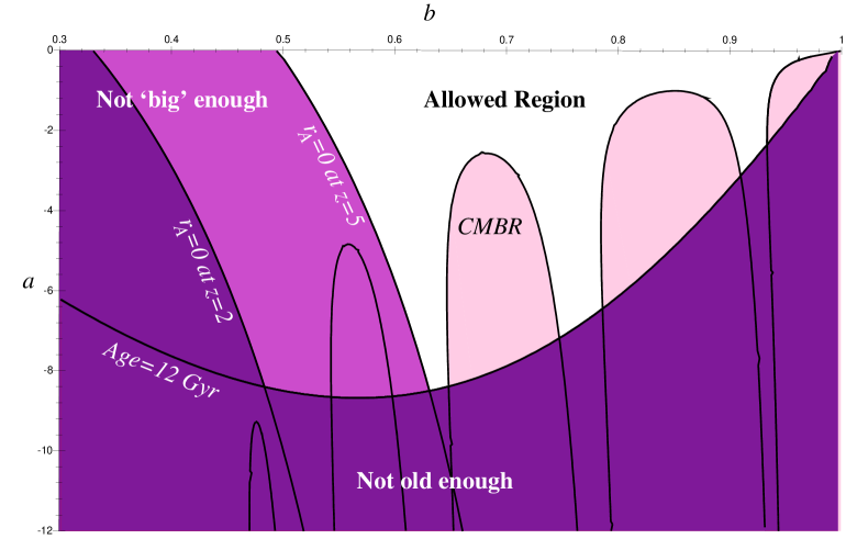
Figure 5.12: The complete exclusion diagram for all the observational constraints studied (age, size and the CMB anisotropy), for $H_{0}=50$ km s^-1 Mpc^-1. We have taken the $12$ Gyr age constraint, to be conservative. The dominant energy condition should be added to these constraints: it eliminates models with $b>0.82$ (equation (5.21)).

we can see that for $H_{0}=50$ km s^-1 Mpc^-1 the strongest constraint comes from the CMB, with age placing somewhat weaker limits on the allowable degree of inhomogeneity (which is measured largely by the size of $a$ – see §5.3). The ‘size’ restriction of §5.2.3 eliminates quite a large region of parameter space for small $b$, but this is not really a constraint on the inhomogeneity, which is our principle concern.

Perhaps rather surprisingly, given the results of Da̧browski and Hendry (1998) and Paper I, the strongest constraint for larger $H_{0}$ really comes from the age. As can be seen in figure 5.13, the exclusion plot for $H_{0}=70$ km s^-1 Mpc^-1,

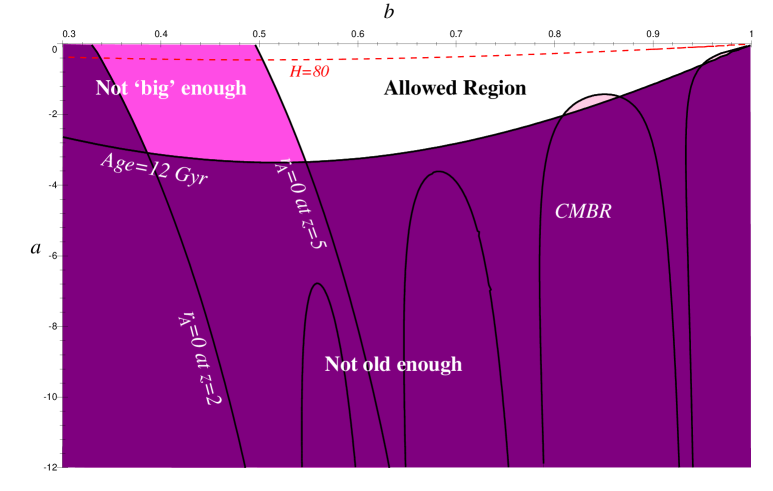
Figure 5.13: As in figure 5.12, but for $H_{0}=70$ km s^-1 Mpc^-1. The age constraint for $H_{0}=80$ km s^-1 Mpc^-1 is also shown as a dashed line (close to the $b$-axis): high $H_{0}$ means a very low age, just as for the FLRW models.

the CMB constraint pokes out in places to eliminate certain regions, and the size constraint cuts off low values of $b$, but age does most of the dirty work. It can also be seen that for $H_{0}=80$ km s^-1 Mpc^-1 age imposes a very strong constraint on the models (dashed line in figure 5.13): the models must be very nearly homogeneous. However, if we relaxed the age constraint to (a probably quite acceptable) $10$ Gyr the CMB anisotropy would be the dominant limitation for most values of $H_{0}$ in the currently fashionable range ($50\mathrel{\vbox{\hbox{\tiny\ooalign{\raise 3.25pt\hbox{$<$}\crcr$\sim$}}}}H_{0}\mathrel{\vbox{\hbox{\tiny\ooalign{\raise 3.25pt\hbox{$<$}\crcr$\sim$}}}}80$ km s^-1 Mpc^-1).

We should not forget, at this point, to reintroduce the restriction (5.21) from the dominant energy condition, which rules out high $b$. This is not shown on the diagrams, in order to avoid clutter. Most of the models eliminated by this constraint have already been ruled out by the age or CMB constraints, and models that are rejected solely by the dominant energy condition are not hugely inhomogeneous (see the next section).

5.3 The Size of the Inhomogeneity.

While we have considered many different aspects of the Da̧browski models, what we have not done is to assess the extent to which the models that are not excluded are inhomogeneous. It is obvious from the exclusion plots, figures 5.12 and 5.13, that the homogeneous Da̧browski models (those with $a=0$) are the ’most acceptable’, in that all the constraints favour small $a$. This should not be surprising, as far as anisotropy constraints are concerned, at least. What is not clear is whether the allowed region only contains models that are very nearly homogeneous. We will show that it does not.

The most natural way to assess the degree of inhomogeneity of the models is to examine the variation of the pressure over surfaces of constant cosmic time. It can be seen from (5.17) that the extremes of pressure occur at $\chi=0$ and $\chi=\pi$, so we define the inhomogeneity factor $\Pi$ to be the relative pressure difference between the two poles:

$$\Pi=\left|\frac{p(\pi)-p(0)}{p(0)}\right|=\frac{8|a|R}{c\Delta}.$$ (5.57)

If $\Pi\mathrel{\vbox{\hbox{\tiny\ooalign{\raise 3.25pt\hbox{$>$}\crcr$\sim$}}}}1$ then it is reasonable to say that the models are truly inhomogeneous, whereas if $\Pi\ll 1$ they are obviously nearly FLRW. Note, though, that $\Pi$ depends on the cosmic time surface under consideration: for small $t$, $\Pi\approx 0$, and $\Pi$ reaches its maximum at $t=-b/2a$ (see (5.3)), at which time

$$\Pi=\frac{2b^{2}}{1-b^{2}}=2\frac{1-\Delta}{\Delta}$$

so that the models are significantly inhomogeneous ($\Pi\mathrel{\vbox{\hbox{\tiny\ooalign{\raise 3.25pt\hbox{$>$}\crcr$\sim$}}}}1$) when

$$b\mathrel{\vbox{\hbox{\tiny\ooalign{\raise 3.25pt\hbox{$>$}\crcr$\sim$}}}}\frac{1}{\sqrt{3}}\approx 0.58.$$ (5.58)

Most of the allowed models in figures 5.12 and 5.13 are unaffected by (5.58) – models with smaller $b$ have already been eliminated by the size constraint in §5.2.3.

This is not really a fair reflection of the inhomogeneity of the models at the times of observation that are relevant here, though, because the $H_{0}$ constraint (5.28) generally ensures that the epoch of observation is quite early on in the evolution of the universe when the scale factor is somewhat smaller than its maximum size. To evaluate the impact of this, consider two specific examples. From the allowed region of (5.12) choose the model at $a=-7$, $b=0.75$. For $H_{0}=50$ km s^-1 Mpc^-1 the solution of (5.28) is $T\approx 0.016$ Mpc s km^-1, which gives $\Pi=1.33$. For the model at $a=-8$, $b=0.64$ we get $T=(3-\sqrt{5})/50\approx 0.015$ Mpc s km^-1 and $\Pi=0.86$, which is close enough to $1$. These models are certainly not ‘close to FLRW’.

Nevertheless, it could be said that the models are not massively inhomogeneous, and that their degree of inhomogeneity only reflects the looseness of the constraints applied. This is not so. Firstly, we have at every stage chosen stronger limits than were strictly necessary, especially as far as the age is concerned, where we could have adopted a $10$ Gyr limit, rather than $12$ Gyr, which would have increased the allowed region considerably. Most importantly of all, though, is the fact that even for models that are only inhomogeneous at the 10% level ($\Pi=0.1$), the CMB anisotropy, $\delta_{1}<10^{-4}$, is at least three orders of magnitude smaller than the inhomogeneity it permits. This certainly conflicts with the spirit of the almost EGS theorem of Stoeger, Maartens, and Ellis (1995) (although not the actuality, since our models have acceleration, whereas the theorem deals with geodesic observers), which says that small CMB anisotropies give rise to small perturbations from homogeneity.

5.4 Fitting to FLRW Models

So far we have demonstrated that the Da̧browski models do not have any problem with regard to the ‘global’ constraints we have considered. As far as ‘local’ constraints are concerned we have only considered the size of the dipole, and ensured it was not too large. We still have to show that the Da̧browski models are capable of providing an acceptable fit to the observed magnitude-redshift relation. A glance at figure 6.14 (with reference to figure 2.4 for the FLRW case) shows that these IRF models are quite capable of producing very incompatable $m-z$ relations. In order to demonstrate that the Da̧browski models are acceptable in this regard we ‘match up’ the Da̧browski $m-z$ relation to the FLRW one. Because of the local dipole considered above we will simply fit the two curves for an observer located at the center. (Obviously a best fit from any location will pick out the center as the location most able to fit the FLRW models.) This should provide confidence, if not conclusive evidence, that the Da̧browski models are acceptable in terms of this test.

The complete solution of fitting the two $m-z$ relations is quite complicated. Given an actual data set it is very easy to decide whether either model is consistent with it: form a $\chi^{2}$ statistic and check whether it is small enough for the model to be consistent at the desired confidence level. To distinguish two theoretical models, however, it is, strictly speaking, necessary to adopt a sort of ‘two-level’ approach and ask: assuming that the Stephani model is the true model of the universe, what is the probability, $\rho_{1}$, that we would, for any realistic data set, reject the FLRW model at some confidence level, $\rho_{2}$? To answer this rigorously requires consideration of all possible data sets drawn from both the FLRW and the Stephani distributions. In fact, we will use a much simpler and more intuitive resolution criterion based on the mean-square difference between the theoretical models. This will be more than adequate for our purposes. For brevity we give a detailed derivation for the $m-z$ relations only, any other case being similar.

The mean-square difference between $m_{S}(z)$ and $m_{F}(z)$ over some $z$-range $0\leq z\leq z_{\mathrm{max}}$, for which we expect to have observations, is

$$D_{2}=\frac{1}{z_{\mathrm{max}}}\int_{0}^{z_{\mathrm{max}}}[m_{S}(z)-m_{F}(z)]^{2}\,dz$$ (5.59)

We assume (as is justifiable for the case we consider here) that the difference $m_{S}(z)-m_{F}(z)$ is smooth and slowly varying, and also that the integral does not need weighted – ie, that the number density is uniform in redshift. Then we imagine that the difference is just a constant; $m_{S}(z)-m_{F}(z)=\sqrt{D_{2}}$. We can accept or reject this difference on the basis of the usual $\chi^{2}$ analysis.

We adopt the null hypothesis that the FLRW model is correct so that the data set consists of $n$ data points $\{m_{i},z_{i}\}$ such that the errors on the $m_{i}$ are normally distributed with variance $\sigma^{2}$ say; ie, $m_{i}=m_{F}(z_{i})+\epsilon_{i}$ where $\epsilon_{i}\sim N(0,\sigma^{2})$. Then, clearly

$$m_{S}(z)-m_{F}(z)=\sqrt{D_{2}}\leq{\frac{\sigma}{\sqrt{n}}}$$ (5.60)

(since $m_{S}(z)-m_{F}(z)=$const. implies the best fit value of $m_{S}(z)-m_{F}(z)$ is $\langle m_{i}-m_{F}(z)\rangle=\langle\epsilon_{i}\rangle$ and the variance on this estimate goes as $\sigma^{2}/n$).

Now, for the SNIa of Perlmutter et al. (1999) $n=42$ and their error on the intrinsic magnitude dispersion is $\sigma\approx 0.15$. This implies

$$D_{2}\leq{\frac{\sigma^{2}}{n}}\approx 5\times 10^{-4}$$

for these data. We take $z_{\mathrm{max}}=1$. When we fit the Stephani to the FLRW model we require $D_{2}\mathrel{\vbox{\hbox{\tiny\ooalign{\raise 3.25pt\hbox{$<$}\crcr$\sim$}}}}10^{-4}$ to demonstrate that the Stephani models are capable of providing at least as good a fit to the SNIa data as an FLRW model.

The procedure we use is to fix $H_{0}$ and $\Omega_{0}$ and find the ‘best fit’ parameters $a,b$ and $T$ for a range of $q_{0}$ (effectively $\Omega_{\Lambda}$). For simplicity we consider two values of $\Omega_{0}=0.3,1.0$. In figures 5.14 to 5.16 we show the best fit values of $a,b$ and $T$ against $q_{0}$. We can see that a negative $q_{0}$ requires $a>0$ as expected from the strong energy condition. In figure 5.17 we show the goodness of fit: provided $D_{2}<10^{-4}$ then these models will fit the SNIa data acceptably. Finally, in figure 5.18 we demonstrate that a positive value of $a$ will enable an old enough universe.

Figure 5.14: The best fit value of $a$ over a range of $q_{0}$ for two values of $\Omega_{0}$.

Figure 5.15: The best fit value of $b$ over a range of $q_{0}$ for two values of $\Omega_{0}$.

Figure 5.16: The best fit value of $T$ (in Gyr) over a range of $q_{0}$ for two values of $\Omega_{0}$.

Figure 5.17: The mean-squared difference as a function of $q_{0}$. Provided this function satisfies $D_{2}<10^{-4}$ then the SNIa data will not be able to distinguish between the FLRW and Stephani models. This is clearly satisfied in these cases.

Figure 5.18: The best fit values of $a$ vs. $T$. This clearly shows that a positive value of $a$ will provide a sufficiently old universe.

5.5 Conclusions.

We have discussed the observational relations and other properties of a family of inhomogeneous perfect fluid cosmological models which, in contrast to FLRW models, have pressure gradients and consequently acceleration of the fundamental observers. It was demonstrated that these models do not suffer from particle horizons (although they also do not contain a radiation field, which, were it to be present, would dominate at early times, leading to a more rapid evolution of the scale factor at early times and the reintroduction of horizons). More importantly, our studies have shown that there is a significant subset of this family that are markedly inhomogeneous but cannot be excluded on the basis of the tests considered here. It is possible, for every observer in each of the models in the allowed regions of figures 5.12 and 5.13, to choose the epoch of observation so that the observed value of $H_{0}$ is reproduced, the age is greater than the measured age of the universe and there are no obviously unacceptable features at low-redshift ($z\mathrel{\vbox{\hbox{\tiny\ooalign{\raise 3.25pt\hbox{$<$}\crcr$\sim$}}}}5$) in the observational relations. It has also been shown that it is possible for these models to reproduce the FLRW magnitude-redshift relation to high accuracy. Most importantly, though, the dipole in the cosmic background radiation would be considerably smaller than the observed CMB dipole: despite the inhomogeneity of the models the anisotropy they produce is very small. The fact that this is true for every observer means that it is not possible to reject these models by appealing to the Copernican principle. As a result, the standard assumption that the observed high degree of isotropy about us combined with the Copernican principle necessarily forces the universe to be homogeneous (the cosmological principle) is seriously undermined.

It is clear from 5.12 and 5.13 that the constraints on the inhomogeneity are much more severe for values of $H_{0}$ at the upper end of the currently accepted range ($H_{0}\mathrel{\vbox{\hbox{\tiny\ooalign{\raise 3.25pt\hbox{$>$}\crcr$\sim$}}}}70$ km s^-1 Mpc^-1), and from the results of §5.2.2 it can be see that a higher age also results in stricter limits. It should be noted, though, that the constraints we have adopted are invariably stronger than is strictly required by observations, so that the results are conservative. Moreover, the principal interest in this thesis is the relationship between anisotropy and inhomogeneity, particularly with regard to the CMB. The fact that age places a strong constraint on the models for large $H_{0}$ is less interesting than the fact that the anisotropy induced in the CMB is smaller for larger $H_{0}$: it seems quite reasonable to believe that it should be possible to find models that are similarly isotropic, though inhomogeneous, but that have much more efficacious age characteristics. In fact when $a>0$, which we require for $q_{0}$ according to the best fits, are much older than their $a<0$ counterparts.

In the following chapter we investigate the properties of the more general $\zeta\neq 0$ models. We will demonstrate that a substantial deviation from spherical symmetry does not cause major problems for the ‘global’ tests we have considered so far. However, the local dipole is large enough to possibly preclude some of these models.

Chapter 6 Observational Characteristics When $\zeta\neq 0$

In chapter 5 we looked into the general observational characteristics of the spherically symmetric Stephani solutions ($\zeta=0$) which admit an isotropic radiation field, with the scale factor $R$ restricted to be a quadratic, and we demonstrated that the models have no significant problems with fitting the broader aspects of our universe. It was also shown that some of the allowed models are significantly inhomogeneous. There is no particular reason for choosing a scale factor of this form, and it is highly likely that the freedom in $R(t)$ could mean that there are even better forms for the scale factor to fit observations. This is a degree of freedom which we do not exploit here.

This chapter is devoted to giving the results for the more general case of $\zeta\neq 0$ (the ‘isotropic radiation field’ or IRF models). The idea is exactly the same as before, but the algebra is a bit more messy. In fact none of the observational relations can be given in analytic form, so graphical methods are used to show that there is a distinctly non-zero ‘volume’ of parameter space that cannot be rejected by current observations.

6.1 Hyperbolic Stephani Models: Overview

We have commented before on the conformal nature of the IRF models, which have allowed us to perform rotations to arbitrary locations in the spacetime. The same conformal nature has allowed us to find all the relevant observational relations for these models. The inhomogeneity of the models is ‘contained’ in the conformal factor $W$. In fact, because the light rays are unaffected by the conformal factor, we see inhomogeneities as they were in the past, which allows the CMB to be so isotropic (the universe is homogeneous at early times.

We have the conformal factor of the metric (4.23)

$$W \!\!\!\!= \!\!\!\!\Phi_{+}+\Phi_{-}\cos\psi\cos\chi-{\frac{2\zeta R}{c\sqrt{\Delta}}}\cos\xi\sin\psi\cos\chi$$ (6.1)

$$\!\!\!\!+ \!\!\!\!\sin\chi\cos\vartheta\sqrt{\Phi_{-}^{2}\sin^{2}\psi+4{\frac{\zeta^{2}R^{2}}{c^{2}\Delta}}(1-\cos^{2}\xi\sin^{2}\psi)+2{\frac{\zeta R\Phi_{-}}{c\sqrt{\Delta}}}\cos\xi\sin 2\psi},$$

where

$$\Phi_{\pm}\!\!\mathrel{\vbox{\hbox{ \ooalign{\raise 4.75pt\hbox{${\textsf{\tiny{\,def}}}$}\crcr$=$}}}}{\frac{1}{2}}\left[1\pm{\frac{\kappa}{\Delta}}+4\zeta^{2}{\frac{R^{2}}{c^{2}\kappa}}\right].$$ (6.2)

We have $\kappa$ restricted by (4.3);

$$\kappa(t)\!\!\mathrel{\vbox{\hbox{ \ooalign{\raise 4.75pt\hbox{${\textsf{\tiny{\,def}}}$}\crcr$=$}}}}{\frac{1}{2}}\Delta-2{\frac{a}{c}}R+2\Sigma_{\pm}\sqrt{\left({\textstyle\frac{1}{4}}\Delta-{\frac{a}{c}}R\right)^{2}+{\frac{\Delta\zeta^{2}}{c^{2}}}R^{2}},$$ (6.3)

where

$$\Sigma_{\pm}\!\!\mathrel{\vbox{\hbox{ \ooalign{\raise 4.75pt\hbox{${\textsf{\tiny{\,def}}}$}\crcr$=$}}}}\hbox{sign}\left({\frac{1}{2}}\Delta-{\frac{2a}{c}}R\right).$$ (6.4)

We take the sign in front of the square root term to be the sign of ${\textstyle\frac{1}{2}}\Delta-2aR/c$ in (4.3) to give the Da̧browski models in the limit $\zeta\rightarrow 0$ whatever the sign of ${\textstyle\frac{1}{2}}\Delta-2aR/c$. We take $R$ to be

$$R(t)=ct(at+b).$$ (6.5)

Note that $\Delta\!\!\mathrel{\vbox{\hbox{ \ooalign{\raise 4.75pt\hbox{${\textsf{\tiny{\,def}}}$}\crcr$=$}}}}1-b^{2}$ and we replaced $\delta\!\!\mathrel{\vbox{\hbox{ \ooalign{\raise 4.75pt\hbox{${\textsf{\tiny{\,def}}}$}\crcr$=$}}}}-a/c$.

The units we will use are as follows: $[c]=$ km s^-1, $\chi,\psi,\xi$ are dimensionless, $R$ is in Mpc and $[t]=$ Mpc s km^-1$=[1/H_{0}]$, so that $[a]=$ km s^-1 Mpc^-1$=[H_{0}]$ and $b$ is dimensionless. Note that we have redefined $\zeta\mapsto\zeta/c$ to give the units of $[\zeta]=[H_{0}]$.

We will now use all the constraints of chapter 5.

6.2 Energy Conditions

As before, we don’t have a specific form of thermodynamic scheme for the IRF models, although chapter 3 proved the existence of one. Knowing the specific form of such a scheme would be desirable, but rather difficult (Sussman, 1999). Rather we wish to limit the models just using the energy conditions:

$$\mu \!\!\!\!\geq \!\!\!\!0$$ (6.6)

$$\mu c^{2}+p \!\!\!\!\geq \!\!\!\!0$$ (6.7)

$$\mu c^{2}+3p \!\!\!\!\geq \!\!\!\!0$$ (6.8)

$$\mu c^{2}-|p| \!\!\!\!\geq \!\!\!\!0.$$ (6.9)

The first must always be satisfied; the second is the weak energy condition, while the other two are the strong and dominant energy conditions respectively. They say that for all reasonable forms of matter the energy density is positive and the pressure cannot be very large and negative; the dominant conditions goes even further and says that positive pressures can’t be large either. For the IRF models we have

$${\frac{8\pi G}{c^{2}}}\mu \!\!\!\!= \!\!\!\!{\frac{3\kappa}{R^{2}}}+{\frac{\theta^{2}}{3c^{2}}}={\frac{3\kappa}{R^{2}}}+{\frac{3R^{2}}{c^{2}\Delta^{2}}}\left[\left({\frac{\kappa}{R}}\right)_{,t}\right]^{2}$$

$$p \!\!\!\!= \!\!\!\!-\mu c^{2}+{\frac{1}{3}}\mu_{,t}c^{2}\left.{\frac{W}{R}}\right/\left({\frac{W}{R}}\right)_{,t}.$$ (6.10)

The conditions are pretty complicated and will not submit to an analytic treatment. We can turn to graphical methods to give a rough guide. It turns out that, as in the Da̧browski case the strong condition requires $a<0$, and the dominant energy condition fails at certain times and places. As in §5.1.1, things are worst when the universe is half way through its evolution, $t=-b/2a$; similarly on one timelike slice the condition will hold in some places (near $\psi=0$) and fail at others ($\psi=\pi$). We test the condition at this spacetime point ($t=-b/2a,~{}\psi=\pi$), on the assumption that if the models are unacceptable there then they will be unacceptable everywhere.

In figure 6.1,

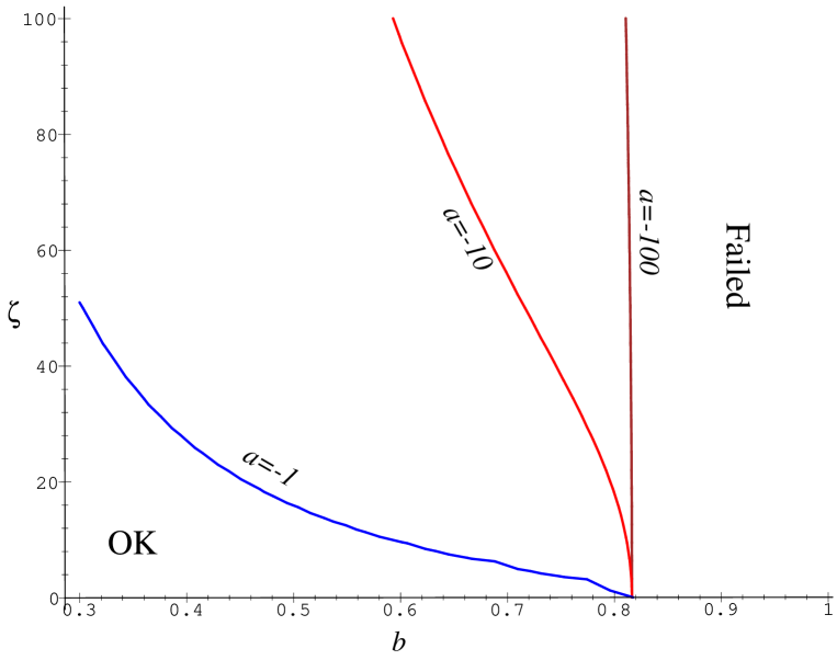
Figure 6.1: Regions of the $b-\zeta$ plane rejected by the dominant energy condition, at $t=-b/2a,~{}\psi=\pi$ for 3 values of $a$. What is surprising is that a small value of $a$ (when $\zeta\neq 0$) rules out more of the $b-\zeta$ parameter space.

we show that a high value of $\zeta$ combined with a small value for $a$ fails the dominant energy condition. As $a$ becomes large and negative, $\zeta$ becomes less and less important, with $b$ being most important for determining the acceptability of the models. As in the case $\zeta=0$, any value of $b\geq\sqrt{2/3}$ is always disallowed.

To try to get a feeling for this, consider figure 6.2,

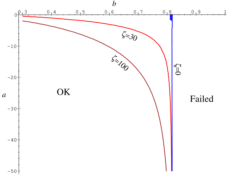
Figure 6.2: Regions of the $a-b$ plane rejected by the dominant energy condition, at $t=-b/2a,~{}\psi=\pi$ for 3 values of $\zeta$. Once again a small value of $a$ (when $\zeta\neq 0$) rules out more of the parameter space.

where we show the same as figure 6.1, but now in the $a-b$ plane. As $\zeta$ becomes large, $a$ must be large and negative or the dominant energy condition will be broken.

The Stephani models have enough problems with their matter content without chastising them for failing this condition. We will banish this problem from our minds, in the knowledge that it actually won’t really matter because, as we will see below, the dominant energy condition doesn’t rule out anything that isn’t more or less ruled out by other conditions. The matter is ‘reasonable enough’ to pass both the weak and strong conditions.

6.3 $H_{0}$

We must have our observers living at a coordinate time which is representative of us. We do this by ensuring that the observers measure a (mean) Hubble’s constant (ie, $\theta/3$) the same as we measure. It will not change over a surface of constant time.

As before, we require the expansion rate to lie somewhere in the range $50\leq H_{0}\leq 80$ km s^-1 Mpc^-1. This means that for any given choice of parameters the age, $T$, of the universe is given by the solution of

$$H_{0}=\left.-{\frac{R}{\Delta}}\left({\frac{\kappa}{R}}\right)_{,t}\right|_{t=T}.$$ (6.11)

For simplicity, in this chapter we take a fixed value of $H_{0}=60$ km s^-1 Mpc^-1, because the added complication of considering a range of $H_{0}$ does not warrant the effort: in chapter 5 the differences were only small. So, for any given values of the parameters $\zeta,a,b$ we have a value of the coordinate age $T$ given by the solution of

$$\left.-{\frac{R}{\Delta}}\left({\frac{\kappa}{R}}\right)_{,t}\right|_{t=T}=60,$$ (6.12)

which is pretty complicated (it’s a sixth order polynomial in $T$).

6.4 Age

It is known that the universe is older than 10 Gyr old, and probably older than 12 Gyr (cf, §5.2.2). The standard model has gone through various crises over this problem, but at the moment things seem to be acceptable, provided that $H_{0}\mathrel{\vbox{\hbox{\tiny\ooalign{\raise 3.25pt\hbox{$<$}\crcr$\sim$}}}}67$ km s^-1 Mpc^-1. We require that any observer in the spacetime, with a local expansion rate $H_{0}=60$ km s^-1 Mpc^-1 be older than 10 or 12 Gyr. The proper age of any observer is given by

$$\tau_{0}\!\!\mathrel{\vbox{\hbox{ \ooalign{\raise 4.75pt\hbox{${\textsf{\tiny{\,def}}}$}\crcr$=$}}}}\int_{0}^{T}{\frac{dt}{W(0,t)}}$$ (6.13)

where $T$ is the solution of (6.12). This integral may have an analytical solution, but we just use a simple numerical analysis, as for all the other tests. To gauge what is going on, in figure 6.3,

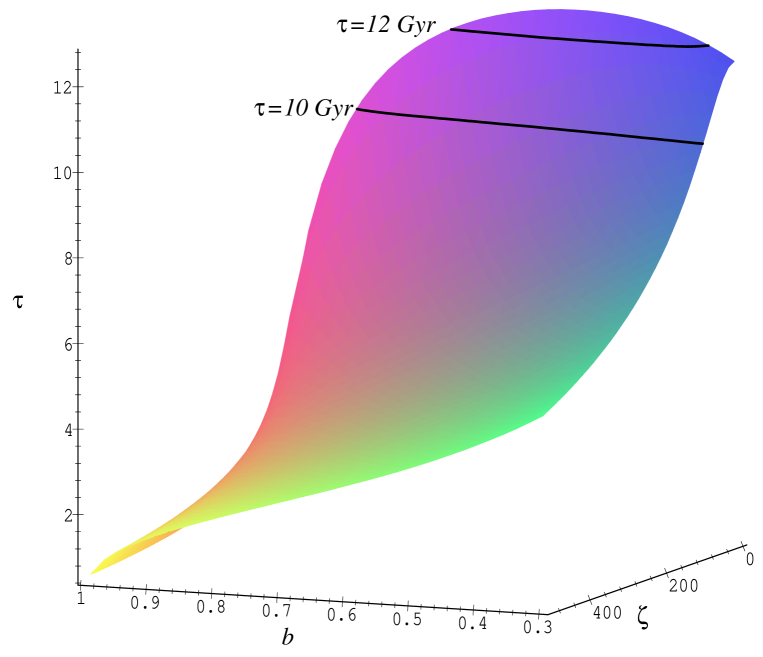
Figure 6.3: Age exclusion plot of $\zeta$ vs $b$ for $a=-5$ and $H_{0}=60$ km s^-1 Mpc^-1 at $\psi=\pi$. The contours mark the limits of the allowed ages.

we show a surface plot of proper age verses $b$ and $\zeta$ for $a=-5$. contours at $10$ and $12$ Gyr are marked on, demonstrating that for high $\zeta$ the age is far too low, for the expansion rate we measure. This means that if we introduce a large $\zeta$ the expansion rate will be too low when the universe is old enough to accommodate globular clusters. This can also be seen in figures 6.5 and 6.6.

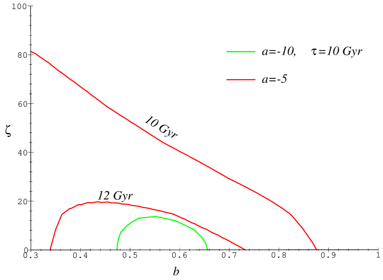
Figure 6.4: Age exclusion plot of $\zeta$ vs $b$ for various $a$ with $H_{0}=60$ km s^-1 Mpc^-1 at $\psi=\pi$. The contours mark the limits of the allowed ages.

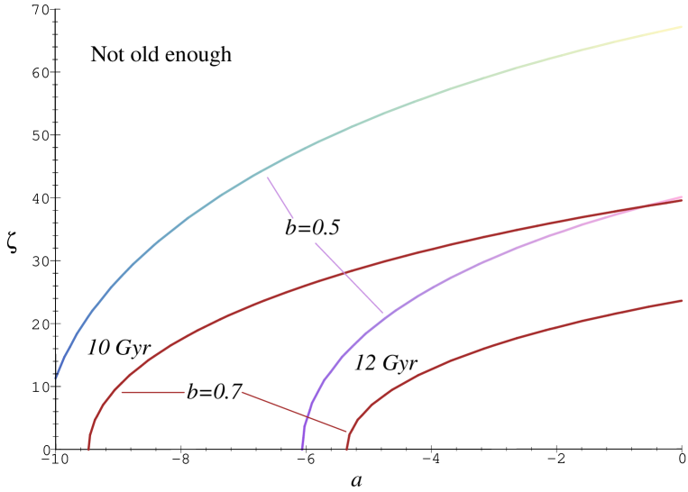
Figure 6.5: Age exclusion plot of $\zeta$ vs $a$ for $a=-5$ and $H_{0}=60$ km s^-1 Mpc^-1 at $\psi=\pi$. The contours mark the limits of the allowed ages. As in the case $\zeta=0$ a large negative $a$ is not allowed by this test.

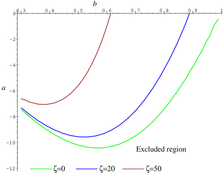
Figure 6.6: Age exclusion plot of $b$ vs $a$ for various values of $\zeta$ and $H_{0}=60$ km s^-1 Mpc^-1 at $\psi=\pi$. These curves are all for an age of $10$ Gyr. Increasing $\zeta$ restricts high values of $b$.

6.5 Area Distance

In §5.2.3 we considered the area distance-redshift relation, with respect to the ‘size’ of the observed spatial sections. This is because the zero in the distance-redshift relation at small redshift, for certain model parameters (namely small $b$), is probably ruled out by present observations. Since the spacetime is conformal to a spherically symmetric spacetime, a zero in $r_{A}(z)$ would correspond to a star situated opposite to an observer (ie, at $\chi=\pi$ for all $\psi$) would become spread all over the observers sky and have an infinite apparent magnitude – it would look as bright as if the star were right next to the observer. Similarly, an object close to a pole would become distorted in a similar manner to normal gravitational lensing – see MacCallum and Ellis (1970) for the distortion formula. As in §5.2.3, we make the assumption that such an effect would have been detected. As before we consider the cases $z_{\pi}\geq 2$ and $z_{\pi}\geq 5$.

To proceed, then, we simply need look at the $z(\chi)$ function at $\chi=\pi$ and at a coordinate age given by (6.12); ie, we must find the range of parameter space for which

$$z(\chi=\pi)\geq 2,~{}\hbox{or}~{}5.$$ (6.14)

We are dealing with a 3-dimensional parameter space so we must proceed with care. In figure 6.7

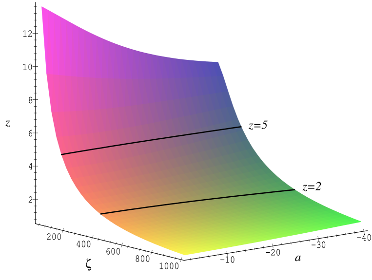
Figure 6.7: Exclusion plot of $\zeta$ vs. $a$ for $b=0.7$ and $H_{0}=60$ km s^-1 Mpc^-1 for the first zero of the $r_{A}(z)$ function.

we show a 3-dimensional plot of $z$ for a variation of the parameters $a$ and $\zeta$, for $b=0.7$. We see from this that for large $\zeta$ the redshift at which the first zero in the $r_{A}(z)$ function occurs at a very low redshift. The second thing to notice is that, even though $a$ varies between $-40$ and $0$ the curves don’t change much. In fact, if we look at figure 6.8,

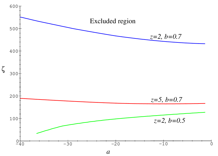
Figure 6.8: Exclusion plot of $\zeta$ vs. $a$ for $b=0.7,0.5$ and $H_{0}=60$ km s^-1 Mpc^-1 for the first zero of the $r_{A}(z)$ function. This clearly shows that only $b$ affects this function significantly.

we see that $a$ doesn’t do much damage at all: $b$ and $\zeta$ seem to be most important. In chapter 5 this was also the case; most of the problems came from small $b$ (cf, fig 5.9). In figure 6.9,

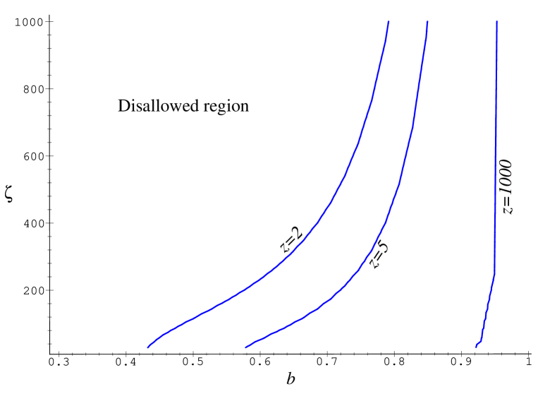
Figure 6.9: Exclusion plot of $\zeta$ vs. $b$ for $a=-10$ and $H_{0}=60$ km s^-1 Mpc^-1 for the first zero of the $r_{A}(z)$ function.

we demonstrate that this is the case: small $b$ is ruled out, while large $\zeta$ is only permitted if $b$ is sufficiently close to 1.

Also in figure 6.9, we show that for the first zero to occur ‘behind the CMB’ requires $b\sim 1$.

In order to understand the effects that $\zeta$ has on the spacetime, we need to study the $a-b$ plane for various values of $\zeta$.

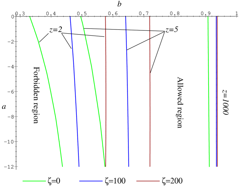
Figure 6.10: Exclusion plot of $a$ vs. $b$ for various values of $\zeta$ for the first zero of the $r_{A}(z)$ function.

In figure 6.10 we show this exclusion plot, from which we can immediately see that a large $\zeta$ has the effect of moving the excluded region towards larger $b$, while at the same time making $a$ more and more redundant as a parameter for this test. Physically the effect of a large $\zeta$ is to decrease the ‘size’ of the spatial sections, as one looks into the past; the first zero in the $r_{A}(z)$ function will occur closer to the observer.

6.6 The CMB Anisotropy

We assume for simplicity that the CMB is a blackbody which occurs at $T=3000$K, which is roughly the temperature of decoupling. As it is a blackbody, the temperature evolves according to (see MacCallum and Ellis 1970)

$$\left.T\right|_{{}_{\mathsf{today}}}={\frac{T_{\scriptscriptstyle{CMB}}}{1+z}}.$$ (6.15)

Our observer at some location given by $\psi$ will measure the temperature of the CMB to be given by

$$T_{o}(\psi,\chi_{\scriptscriptstyle{CMB}},\vartheta)={\frac{T_{\scriptscriptstyle{CMB}}}{1+z(\psi,\chi_{\scriptscriptstyle{CMB}},\vartheta)}}.$$ (6.16)

Now from (4.29) and (4.24) we may write

$$1+z(\psi,\chi_{\scriptscriptstyle{CMB}},\vartheta)=1+z_{0}(\psi,\chi_{\scriptscriptstyle{CMB}})+z_{1}(\psi,\chi_{\scriptscriptstyle{CMB}})\cos\vartheta,$$ (6.17)

where

$$1+z_{0} \!\!\!\!\!\!\mathrel{\vbox{\hbox{ \ooalign{\raise 4.75pt\hbox{${\textsf{\tiny{\,def}}}$}\crcr$=$}}}} \!\!\!\!{\frac{R_{0}}{W_{0}R_{\scriptscriptstyle{CMB}}}}\left\{\Phi_{+_{\scriptscriptstyle{CMB}}}+\Phi_{-_{\scriptscriptstyle{CMB}}}\cos\psi\cos\chi_{\scriptscriptstyle{CMB}}\right.$$ (6.21)

$$\hfill\left.-{\frac{2\zeta R_{\scriptscriptstyle{CMB}}}{c\sqrt{\Delta}}}\cos\xi\sin\psi\cos\chi_{\scriptscriptstyle{CMB}}\right\},$$

$$z_{1} \!\!\!\!\!\!\mathrel{\vbox{\hbox{ \ooalign{\raise 4.75pt\hbox{${\textsf{\tiny{\,def}}}$}\crcr$=$}}}} \!\!\!\!{\frac{R_{0}\sin\chi_{\scriptscriptstyle{CMB}}}{W_{0}R_{\scriptscriptstyle{CMB}}}}\left\{\Phi_{-_{\scriptscriptstyle{CMB}}}^{2}\sin^{2}\psi+4{\frac{\zeta^{2}R_{\scriptscriptstyle{CMB}}^{2}}{c^{2}\Delta}}(1-\cos^{2}\xi\sin^{2}\psi)\right.$$ (6.25)

$$\hfill\left.+2{\frac{\zeta R_{\scriptscriptstyle{CMB}}\Phi_{-_{\scriptscriptstyle{CMB}}}}{c\sqrt{\Delta}}}\cos\xi\sin 2\psi\right\}^{{\frac{1}{2}}},$$

where $`X_{\scriptscriptstyle{CMB}}$’$\equiv`X(t(\chi_{\scriptscriptstyle{CMB}}))$’. The multipole moments in the CMB temperature fluctuations will then become

$$T_{\mathrm{obs}}(\vartheta)=\frac{T_{\mathrm{dec}}}{1+z_{0}}\left[1-\frac{z_{1}}{1+z_{0}}\cos\vartheta+\left(\frac{z_{1}}{1+z_{0}}\right)^{2}\cos^{2}\vartheta+{\cal O}(\cos^{3}\vartheta)\right],$$ (6.26)

that is,

$$\frac{\delta T(\vartheta)}{T}=-\frac{z_{1}}{1+z_{0}}\cos\vartheta+\left(\frac{z_{1}}{1+z_{0}}\right)^{2}\cos^{2}\vartheta+O(\cos^{3}\vartheta).$$ (6.27)

The strategy is then as follows:

1. Given a set of parameters, $a,b,\zeta,\xi,\psi$ we solve (6.12) for the coordinate age $T$.

2. Given our complete parameter set $a,b,\zeta,\xi,\psi,T$ we then find the mean distance to the CMB surface $\chi_{\scriptscriptstyle{CMB}}$ by solving

   $$z_{0}(\chi_{\scriptscriptstyle{CMB}})=1000$$ (6.28)

   for $\chi_{\scriptscriptstyle{CMB}}$. This must be done numerically because the equations are such a mess.

3. We can then calculate the temperature anisotropy by calculating $z_{1}$ using the value of $\chi_{\scriptscriptstyle{CMB}}$ found above. The dipole moment of the CMB temperature is then (using (6.17))

   $$\delta_{1}=\frac{z_{1}}{1+z_{0}}\approx 10^{-3}z_{1}.$$ (6.29)

We do not wish that the IRF models account for the entire dipole moment of the CMB, because there is good evidence that this is due to our peculiar velocity of the local group. However, there is no reason to say that a small part of the dipole cannot be of a cosmological origin: a variation of $10\%$ of the dipole could in principle be of a cosmological nature. We take this constraint here; that is $\delta_{1}\sim 10^{-4}$, or $z_{1}\sim 0.1$.

So, that’s the plan. We are principally interested in the effects a non-zero $\zeta$ will have. In figure 6.11

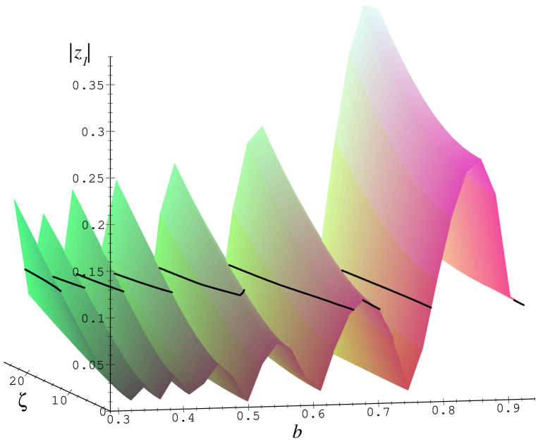
Figure 6.11: Exclusion plot of $\zeta$ vs. $b$ for $\psi=1/4\pi$ for the CMB anisotropy. $a=-5$. Regions below the black contour is acceptable.

we show a surface plot of $|z_{1}|$ against $b$ and $\zeta$. The contour $z_{1}=0.1$ is shown, with the surface below this line representing the acceptable parameter range. This is for an observer at $\psi=\pi/4$. We wish to constrain the parameters from the most restrictive position; it is not obvious, when $\zeta\neq 0$ where the ‘worst’ position is. Figure 6.12

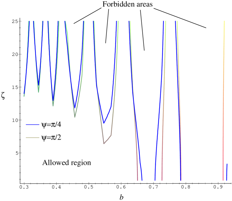
Figure 6.12: Exclusion plot of $\zeta$ vs $b$ for two values of $\psi$ for the CMB anisotropy. $a=-5$.

demonstrates that the most restrictive position for this test is an observer at $\psi=\pi/2$, and we can use that in what follows.

The other thing to notice in figure 6.12 is that $\zeta$ behaves very much as $a$ does in §5.2.4 (cf. Fig. 5.11), that is the excluded regions are ‘fingers’, with the position depending on $b$, and the size depending on $\zeta$.

In figure 6.13,

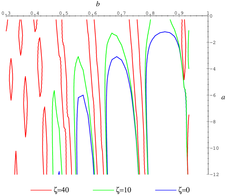
Figure 6.13: Exclusion plot of $a$ vs $b$ for three values of $\zeta$ for the CMB anisotropy. As $\zeta$ increases, the ‘fingers’ move in to exclude more and more of the $a-b$ plane, leaving a few narrow strips and isolated pockets.

we show the exclusion plot in the $a-b$ plane, as in figure 5.11, but for different values of $\zeta$. As can be seen, a high value of $\zeta$ is not exactly ‘ruled out,’ but makes things more ‘unlikely’ to fit. For any value of $a$, the range of allowed $b$ decreases its total size, but never (except for very high $\zeta$) rules out the models completely. This is in contrast to the other constraints, such as the size constraint, which completely rules out small values of $b$; or the age constraint, which rules out large negative values of $a$. Note that all the plots don’t quite get close to $b=1$, as the calculation becomes very (computationally) difficult there; it should be clear from the previous chapter that this region is ruled out.

6.7 The Magnitude-Redshift Relation

Due to the complexity of the equations – basically the conformal factor – a proper analysis of the local inhomogeneity is really beyond the scope of this thesis, although not impossible in principle. Instead we will consider some examples to get an idea of the effect a large value of $\zeta$ will have. It is perhaps appropriate to use the magnitude-redshift relation for this purpose, because it is easier to compare with observations.

To recap, we have

$$m(z)-M-25=5\log_{10}r_{L}=5\log_{10}{\frac{R_{0}}{\sqrt{\Delta}W_{0}}}+5\log_{10}\left\{(1+z)|\sin\chi(z)|\right\},$$ (6.30)

where $\chi(z)$ is given by the solution of

$$1 \!\!\!\!+ \!\!\!\!z(\chi)={\frac{R_{0}}{W_{0}R(\chi)}}\left\{\Phi_{+}(\chi)+\Phi_{-}(\chi)\cos\psi\cos\chi-{\frac{2\zeta R(\chi)}{c\sqrt{\Delta}}}\cos\xi\sin\psi\cos\chi\right.$$ (6.31)

$$\!\!\!\!+ \!\!\!\!\left.\sin\chi\cos\vartheta\left[\Phi_{-}(\chi)^{2}\sin^{2}\psi+4{\frac{\zeta^{2}R(\chi)^{2}}{c^{2}\Delta}}(1-\cos^{2}\xi\sin^{2}\psi)\right.\right.$$

$$\hfill\left.\left.+2{\frac{\zeta R(\chi)\Phi_{-}(\chi)}{c\sqrt{\Delta}}}\cos\xi\sin 2\psi\right]^{{\frac{1}{2}}}\right\},$$

with $R(\chi)\equiv X(t(\chi))$, etc.

We note first of all in figure 6.14,

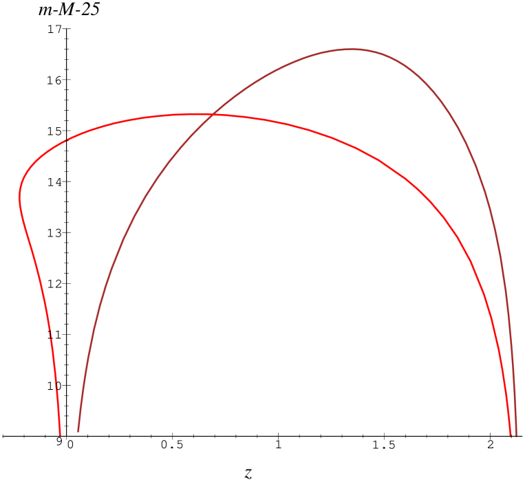
Figure 6.14: The magnitude-redshift relation in opposite directions in the sky for an observer at $\psi=0$. We have $b=0.5,a=-10$, and $\zeta=100$.

we can see that a large $\zeta$ can cause all sorts of problems, with the situation illustrated in figure 6.14 being completely ridiculous. It is not all the fault of $\zeta$ though, as figure 6.15,

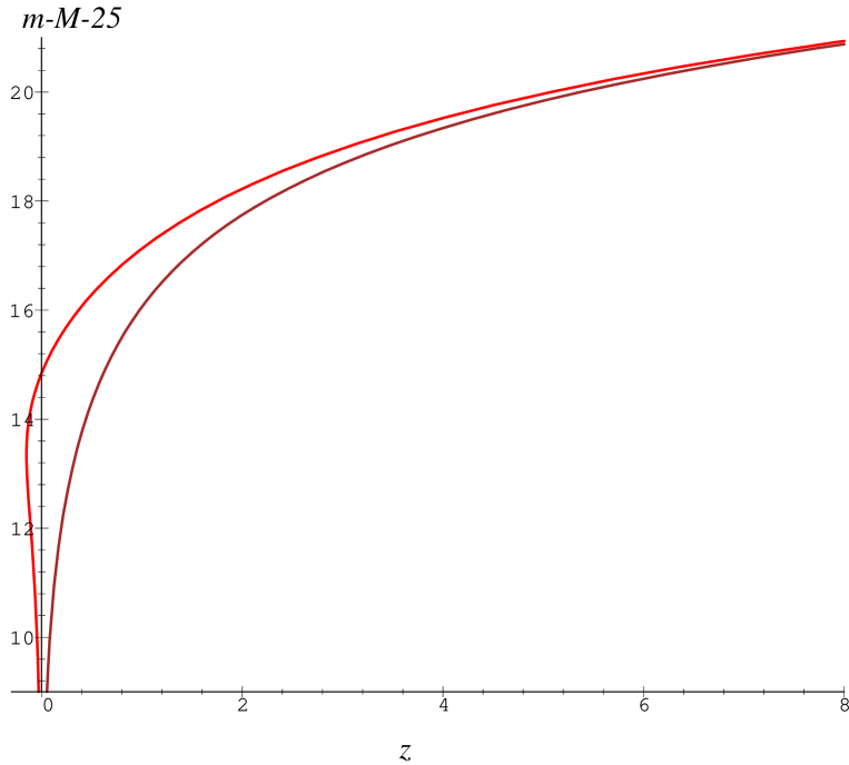
Figure 6.15: The magnitude-redshift relation in opposite directions in the sky for an observer at $\psi=0$. We have $b=0.95,a=-10$, and $\zeta=100$.

demonstrates. A much higher value of $b$ is used, and the problem is slightly relieved. However, the situation is still unacceptable as a cosmological model. It is clear that a blueshift in one direction in the sky is not reasonable – the results are similar whatever the observers location in the spacetime, $\psi$. However the results do depend on $\xi$; with $\xi=\pi/2$ (as all the graphs here have) we get a large dipole moment, which virtually disappears when $\xi=0$. This is because when $\zeta$ is large, the dominant part of the dipole in $1+z$ comes from the second term in the square root.

A far more reasonable situation is shown in figure 6.16,

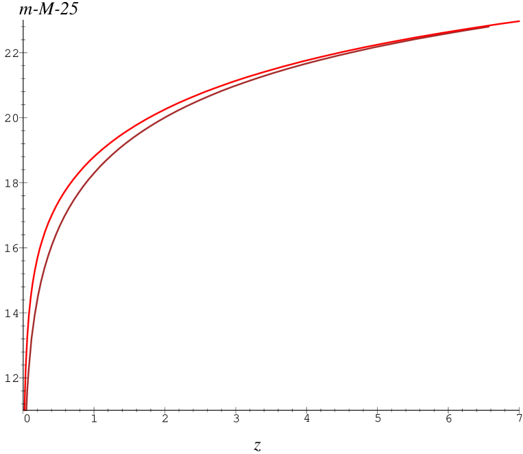
Figure 6.16: The magnitude-redshift relation in opposite directions in the sky for an observer at $\psi=\pi/2$. We have $b=0.9,a=-5$, and $\zeta=5$.

with a much smaller $\zeta$. The observers location is at $\psi=\pi/2$, with the direction to the center given by $\xi=\pi/2$, which seems to be the ‘worst case’ scenario.

The moral seems to be to have $\zeta$ and $|a|$ quite small, and at the same time $b$ should be ‘close to’ 1. It is interesting though, that when $\zeta$ is distinctly non-zero, the dipole in the magnitude-redshift relation is more or less the same regardless of the observers spatial location, but does depend heavily on their direction to the center.

6.8 Summary

It this chapter we have considered the effects of a non-zero $\zeta$. We have shown that the age may be high enough, the first zero of $r_{A}(z)$ does not occur too close to the observer, and that the CMB anisotropies are not too large, for non-zero values of $\zeta$. However, we have shown that a large value of $\zeta$ will introduce a significant dipole into the magnitude-redshift relation. This is probably enough to rule out these models, unless $\xi$ is close to 0: this would violate the Copernican principle. This deserves further consideration.

Chapter 7 Conclusions and Future Work

This thesis has examined the application of the Copernican principle in inhomogeneous spacetimes. The class of models we considered were derived in chapter 3 under the condition that they admit an isotropic radiation field, and were shown to be a subclass of the Stephani solutions with symmetry. A cosmological model which satisfies the Copernican principle must satisfy Theorem 1, if one wants a spacetime with observers who see an (exactly) isotropic CMB. The IRF models we derive are generalisations of the FLRW models, that satisfy Theorem 2 of Ehlers, Geren and Sachs (1966). It was also demonstrated that the models we find all admit a thermodynamic scheme. The rest of the thesis was spent developing the relevant observational relations, and ‘testing’ various aspects of them.

In chapter 4, we derived all the necessary cosmological tests. After the conformal symmetries were recognised, and the relevant coordinate transformations were made, this became a tractable problem. Indeed this transformation enabled us to ‘rotate’ the origin of coordinates to an arbitrary location, which gave the opportunity to derive all the observational relations valid for all observers in the spacetime. This is clearly crucial for the subsequent observational consideration of the Copernican principle.

It chapters 5, and 6, we discussed observational constraints. We limited the coordinate time of observation using the present constraints on $H_{0}$ by constraining the expansion rate with (5.29) and (6.12). For any choice of parameters this gave a value of the coordinate $T$. We then proceeded to examine the models on a variety of tests; the most important being age and the anisotropy of the CMB. Obviously, any plausible cosmological model must have reached the required age by the time the expansion has slowed to the rate we measure today. This is position dependent; on a given surface of constant coordinate time (determined by the expansion rate) the observers at the center will generally be older than their counterparts away from the center (cf, figure 5.4). As with all the tests, we consider only the ‘worst case’ observer position; ie, that which excludes most of the parameter space.

The CMB is also a crucial test. Despite the fact that the IRF models admit an isotropic radiation field by definition, they do not exhibit an exactly isotropic CMB. This is because the models are homogeneous at the big bang $t=0$, or $W=1$ (and big crunch, incidentally), which is when the isotropic radiation field in question is ‘emitted’. The CMB is not emitted then, but a short time after when the universe was inhomogeneous, but not drastically so. The anisotropies in the observed temperature are $\propto 1/(1+z)\sim 1/W$: that is all anisotropies arise from the inhomogeneities in $W$ at the time of emission, and have nothing to do with the subsequent evolution and motion of observers. This means that, since $t$ is small, $W\sim 1$, and the inhomogeneities are very small too; the conformal flatness of the spacetime allows the light from the CMB surface to travel unmolested by any subsequent deviation from homogeneity, and we can see the CMB as a reflection of the universe’s inhomogeneity as it was at that time. The dipole moment of the CMB is the largest moment, which we restrict to be smaller than 10% of the observed dipole, on the assumption that we are unable to say, at present, that the dipole is entirely due to the motion of the local group.

The other tests we considered were that the energy conditions are satisfied (see below) and that the first zero of the $m-z$ relation does not occur too close to the observer. Both these tests are independent of observer location. As we have discussed, these do not impose strong constraints on the available parameter space.

The IRF models we chose to look at had the scale factor (arbitrarily) restricted to be a quadratic function of time. We must conclude, therefore that the allowed degree of freedom in the IRF models, which manifests itself in the freedom in choosing the scale factor, $R(t)$, gives us an enormous range of models which would satisfy the constraints chosen here to a perfectly acceptable level. In fact chapters 5, and 6 may be considered as an existence ‘proof’ that the IRF models are acceptable models of the universe on observational grounds; that their matter content is unappealing does not enter into it.

7.1 A Note On ‘Best Fits’ and $a>0$

The discussion in chapters 5 and 6 is obviously not complete. We should really provide a fit of the $m-z$ relation to real data. However, this would not be simple in general, because any result would be position dependent. Moreover, because of the dipole mentioned above, the data would have to include the directional coordinates of the SNIa. As the complete SNIa data is yet to be made public, we are not able to do this as yet.

However, in the spherically symmetric case, an observer at the center would see no dipole variation of the $m-z$ relation, so it is of value to fit the models from this special location, if only to show a proper fit (ie, as good a fit as may be obtained with an FLRW model) is possible. In §5.4 we demonstrated that this was possible. In fact it is possible to show that any FLRW $m-z$ relation may be ‘matched’ by a suitable choice of parameters in these IRF models (Barrett and Clarkson, in preparation), for an observer at the center.

It should be clear from the discussion in the introduction on the active gravitational mass, that a fit to an FLRW model with $q_{0}<0$ will violate the strong energy condition. This means that local observations at the center will force $a>0$ (cf, §5.1.1). Moreover, we have seen from §5.2.1, that requiring the normalised energy density to be less than unity today also requires $a>0$. This implies that this thesis is incomplete. As we have noted before, $a>0$ implies that the universe will open up at $t=(1-b)/2a$ (in the spherically symmetric case), after which the universe will become infinite in spatial extent. Spatial infinity, in terms of $\psi$ this will happen at $W=0$ (cf, 5.10);

$$\sin^{2}{\frac{\psi_{{}_{\mathsf{max}}}}{2}}={\frac{c\Delta}{4aR(t)}}<1~{}~{}~{}\hbox{for}~{}~{}~{}t>{\frac{1-b}{2a}}.$$ (7.1)

Applying the Copernican principle in this case becomes difficult – at least in terms of producing exclusion diagrams. It may not be possible to find a ‘worst case’ observer position, as we have done up to now. If we choose any $\psi<\psi_{{}_{\mathsf{max}}}$, then the number of observers between the center and $\psi$ will be finite; whereas, between $\psi$ and $\psi_{{}_{\mathsf{max}}}$ the number will be infinite. Thus it is impossible to say that for any $\psi$ we have considered all or most observers.

However, it may be possible to take a constraint, say the CMB dipole, and consider the limit $\psi\rightarrow\psi_{{}_{\mathsf{max}}}$. That is we may say that if

$$\lim_{\psi\rightarrow\psi_{{}_{\mathsf{max}}}}\left|z_{1}\right|<0.1$$ (7.2)

then the model will pass the test, and satisfy the Copernican principle.

This however, is a computational nightmare – as we take the limit, at any given $\psi$, we must solve (6.21) for $\chi_{\scriptscriptstyle{CMB}}$. This must also be done over the whole 3-dimensional parameter space. This is a chore for the future.

7.2 The Local Dipole

The most interesting question this thesis has raised is the possibility that we may be living in a distinctly inhomogeneous universe (that is, not a slightly inhomogeneous perturbed FLRW universe).

Acceleration makes the IRF models inhomogeneous, but will leave its mark in the local universe. This is testable (§3.3) by considering the local dipole moment of $H_{0}$ – ie, the local dipole in the linear Hubble law. The measured dipole is usually interpreted as our peculiar velocity with respect to the CMB frame; that the directions of our peculiar motion from local studies and that of the CMB frame line up to within about $20^{\circ}$ (Saunders et al., 1999; Scaramella et al., 1991; Riess, 1999) lends support to this but it cannot be conclusive. It should be noted that in the IRF models, we also require the local and CMB dipoles to line up.

If we wish to prove homogeneity then we must test this local dipole to determine if it grows linearly with distance. If it does then we may use the slope of this linear relationship to either (cf, 5.32): 1. determine the maximum inhomogeneity of the universe, assuming we are located at or near the ‘equator’ ($\psi=\pi/2$); or, 2. determine our distance from the center, in an arbitrarily inhomogeneous model. Both would require violation of the Copernican principle to some degree. The first would require us to be situated at the point of maximal inhomogeneity (maximum acceleration) – which is a ‘non-typical’ location; while the second may violate it depending on how inhomogeneous we may decide the universe to be. That is, the more inhomogeneous the model (the greater the acceleration at the equator) the closer we must be to the center, and we would no longer be representative of ‘most’ observers.

Preliminary investigations reveal that constraints on the dipole in $H_{0}$ are weak – around 20% may be attributed to an acceleration term (Clarkson, Rauzy, and Barrett, in preparation). This has been investigated using the IRAS galaxy catalogue; however, the recently released PSCz catalogue with around 15000 galaxies may provide stronger constraints.

7.3 Almost EGS Considerations

One may expect that the IRF models derived in §3.1 would extend to an ‘almost’ theorem, in the same manner as the almost EGS theorem of Stoeger, Maartens and Ellis (1995). If we take an almost isotropic radiation field characterised by

$$\sigma_{ab}={\cal O}(\epsilon),$$ (7.3)

$$\nabla_{[a}\left(\dot{u}_{b]}-{\textstyle\frac{1}{3}}\theta u_{b]}\right)={\cal O}(\epsilon),$$ (7.4)

where epsilon is small in some sense then we may write, from equations (3.3)

$$\dot{\mu}_{\!{}_{R}}+{\frac{4}{3}}\theta\mu_{\!{}_{R}} \!\!\!\!= \!\!\!\!{\cal O}(\epsilon)$$

$$4\mu_{\!{}_{R}}\dot{u}_{a}+\widetilde{\nabla}_{a}\mu_{\!{}_{R}} \!\!\!\!= \!\!\!\!{\cal O}(\epsilon),$$ (7.5)

or

$$\dot{u}_{a}=-{\textstyle\frac{1}{4}}\widetilde{\nabla}_{a}\ln\mu_{\!{}_{R}}+{\cal O}(\epsilon)$$ (7.7)

which gives

$$\widetilde{\nabla}_{[a}\dot{u}_{b]}\sim\widetilde{\nabla}_{[a}\widetilde{\nabla}_{b]}\mu_{\!R}\sim\omega_{ba}\theta\neq{\cal O}(\epsilon):$$ (7.8)

there doesn’t seem to be any way to make the rotation small, unless one artificially introduces additional assumptions. Therefore perfect fluid solutions which admit an almost isotropic radiation field may not (at first sight at least) be perturbations of the IRF models. However, there may be ways to constrain rotation on the basis of local observations: rotation leads to anisotropic number-counts – see Fennelly (1976). It would seem unlikely that such observations would be anywhere near as accurate as those of the CMB anisotropies; ie, we would be unable to claim that $\omega_{ab}={\cal O}(\epsilon)$ from number-counts alone.

7.4 Further Considerations

The IRF models, by definition, admit an isotropic radiation field. As all observers see such a radiation field to be isotropic, the isotropy of the CMB cannot be used to verify the cosmological principle. The usual suggestions of testing the cosmological principle directly, necessarily involve making measurements within our past lightcone. The Sunyaev-Zel’dovich (SZ) effect is often quoted as a suitable physical effect to produce such a test (Goodman, 1995). Such a test will involve measuring the anisotropy of the CMB around other observers. It is normally assumed that if the anisotropy is small around other observers then one may conclude that we are not at a special location (eg, at a center of symmetry), and that the universe is FLRW – hence the cosmological principle is verified.

This, of course, assumes that the acceleration is zero. The IRF models would also give the same effect; measurement of the CMB anisotropies as seen by another observer would be similarly small, but these would not imply that the universe is homogeneous, by Theorem 3. Hence, contrary to popular belief, the SZ effect cannot possibly show that the cosmological principle is a valid assumption.

Clearly, the SZ effect cannot distinguish between different IRF models – thus the acceleration may be arbitrarily large. This means that the Copernican principle may be violated, because for our local dipole to be so small (at most 20% of $H_{0}$) would necessarily require us to be close to the center of such an inhomogeneous universe. Therefore the SZ effect will not even be able to provide any proof of the Copernican principle.

It should be noted that acceleration would leave a small signature in such CMB measurements: small dipoles around other observers would be correlated, rather than a random distribution of dipoles from their peculiar motions. The distribution of the dipoles would be a mixture of some pointing in one direction, and others pointing in the opposite direction. In the spherically symmetric case, the direction of the dipole would depend on the number of times the scattered light had passed through the point opposite to us. This will depend on the redshift of the galaxy. It is not clear what pattern the more general IRF models would give.

If we used the SZ effect and found such a pattern of dipoles, then this would imply that acceleration is present in the universe. Such accuracy for these experiments is a long way off, as it would be next to impossible to disentangle any dipole from peculiar velocities and that from acceleration – we have enough difficulty in determining our own.

This poses some interesting questions. It would be interesting to carry on this work along the lines of Stoeger, Maartens and Ellis (1995), and Maartens, Ellis and Stoeger (1995), which is to place limits on all the components which characterise a cosmological model: $\{\dot{u}^{a},\theta,\sigma_{ab},\omega_{ab},E_{ab},\&H_{ab}\}$, together with the matter content. In general this is not a simple task and, as this thesis makes clear, one cannot rely on the CMB alone.

Appendix A Coordinate transformations and the Stephani Spacetimes.

On the face of it the Stephani models admitting an isotropic radiation field in (3.19) depend on one free function and ten free parameters. However, it is possible to use coordinate transformations on the spacetime to eliminate many of these parameters, resulting in a considerable simplification. As is shown in Barnes (1998), conformal transformations of the coordinates on the hypersurfaces of constant time preserve the form of the metric but change the free functions $a$, $b$, and $\mathbf{c}$. These transformations can be thought of as acting on the five-dimensional space spanned by $a$, $b$ and ${\mathbf{c}}$ and constitute the Lorentz group in five dimensions, $SO(4,1)$: they leave $-ab+|{\mathbf{c}}|^{2}$ invariant ($a$ and $b$ are ‘null coordinates’). It will be convenient here to let $a=\alpha+\beta$ and $b=\alpha-\beta$ (so that the transformations preserve $-\alpha^{2}+\beta^{2}+|{\mathbf{c}}|^{2}$), and to adopt five-vector notation: $q^{\mu}=(\alpha,\beta,{\mathbf{c}})$. We will use the terms ‘rotation’ and ‘boost’ to refer to the transformations on $q$, and will call $q$ timelike, spacelike or null if $-\alpha^{2}+\beta^{2}+|{\mathbf{c}}|^{2}$ is negative, positive or zero, as usual. Then it is easy to visualise the transformations on the free functions by imagining the ‘mass hyperboliods’ of representations of the Lorentz group in the usual way: a timelike vector can always be boosted so that it has the form $(\alpha,0,{\mathbf{0}})$, whereas a spacelike vector can be boosted and rotated into $(0,\beta,{\mathbf{0}})$, for example.

In addition to the Lorentz transformations we also have the freedom to change basis in the function space spanned by the free functions. For the spacetimes of interest here, described by (3.19), it is desireable to preserve $f_{2}(t)=1$, so that the basis change is

$$T\mapsto\gamma T+\delta.$$ (A.1)

In five-vector notation the equations (3.19) become

$$q^{\mu}(t)\equiv(\alpha,\beta,{\mathbf{c}})=q_{1}^{\mu}T(t)+q_{2}^{\mu}$$ (A.2)

(with $q_{1}$ and $q_{2}$ constant vectors), and the goal is to reduce as many of the components of $q_{1}^{\mu}$ and $q_{2}^{\mu}$ to zero as possible using Lorentz transformations in the five-dimensional space containing $q_{1}$ and $q_{2}$, and the basis change (A.1). Note that the FLRW ($d=1$) subcase of (3.19) is characterised by the linear dependence of $q_{1}$ and $q_{2}$.

It is easy to see that ${\mathbf{c}}$ (which breaks the spherically symmetry of the metric (3.6)) may always be reduced to the form ${\mathbf{c}}=c{\mathbf{\hat{z}}}$ (${\mathbf{\hat{z}}}=(0,0,1)$), with $c$ a constant: perform a spatial 4-rotation to reduce $q_{1}^{\mu}$ to $q_{1}^{\mu}=(\alpha_{1},\beta_{1},{\mathbf{0}})$, then a spatial rotation amongst the ${\mathbf{c}}$-components (which obviously leaves $q_{1}$ unaffected) to give $q_{2}^{\mu}=(\alpha_{2},\beta_{2},c{\mathbf{\hat{z}}})$.

It is possible in general to make further simplifications, but precisely how $q_{1}$ and $q_{2}$ are simplified depends on whether they are spacelike, timelike or null. For example, if either $q_{1}$ or $q_{2}$ is timelike (or may be made timelike by a transformation (A.1)) it is possible to reduce the model to manifestly spherically symmetric form ($c=0$): boost so that the timelike vector, say $q_{1}$, becomes $q_{1}=(\alpha_{1},0,{\mathbf{0}})$ and rotate spatially so that the ${\mathbf{c}}$-components of the other vector are also zero, $q_{2}=(\alpha_{2},\beta_{2},{\mathbf{0}})$ (we could then use (A.1) to eliminate more of these constants).

To summarise, we have demonstrated that it is always possible to reduce the Stephani models of (3.19) to the form

$$a(t) \!\!\!\!= \!\!\!\!a_{1}T(t)+a_{2},$$

$$b(t) \!\!\!\!= \!\!\!\!b_{1}T(t)+b_{2},$$ (A.3)

$${\mathbf{c}}(t) \!\!\!\!= \!\!\!\!c{\mathbf{\hat{z}}},$$

(where we have transformed back from $\alpha$ and $\beta$ to $a$ and $b$), and when either of the $q_{1}$ or $q_{2}$ is (or may be made) timelike we can set $c=0$.

Finally, note that we may always assume that $a_{1}\neq 0$ in (A.3), because if $a_{1}=0$ then $b_{1}\neq 0$, otherwise $V_{,t}=0$, and it is possible to perform a coordinate inversion ${\mathbf{x}}\mapsto{\mathbf{x}}/r^{2}$ that interchanges $a$ and $b$). This does not exhaust the possibilities for simplification: we could, for example, use (A.1) to set $a_{2}=0$.

Appendix B Transformation to a Non-Central Position.

We want to transform from the $(\chi,\theta,\phi)$ coordinate system, whose origin is at the centre, to coordinates centred instead on some observer at $\chi=\psi$, while preserving the form of the FLRW part of the metric (4.9). It is therefore necessary to identify the transformations of the (homogeneous) FLRW spatial sections that leave the FLRW metric invariant, ie, the isometries of the spatial sections. This is simple. Since the spatial sections of an FLRW model with positive curvature constant ($\Delta>0$) are 3-spheres, the isometries we require are 4-dimensional rotations (ie, elements of $SO(4)$, the isometry group of the 3-sphere).

A sphere of radius $R$ in 4-dimensional space with cartesian coordinates $(x,y,z,u)$ is defined by

$$x^{2}+y^{2}+z^{2}+u^{2}=R^{2}.$$

We have three coordinates on this sphere: $\chi$ and the two spherical polar angles $\theta$ and $\phi$. These are related to the cartesian coordinates by

$$x = R\sin\chi\sin\theta\cos\phi$$ (B.1)

$$y = R\sin\chi\sin\theta\sin\phi$$ (B.2)

$$z = R\sin\chi\cos\theta$$ (B.3)

$$u = R\cos\chi$$ (B.4)

The origin, $\chi=0$, is then at $x=y=z=0$, $u=R$. We are only interested in rotations that move the origin, and, as the initial metric is spherically symmetric (really spherically symmetric, not just conformally: even the conformal factor is spherically symmetric about the centre), we need only consider moving the observer in one direction, which we choose to be the ‘$z$ direction’ (ie, to a position with non-zero $z$, but $x=y=0$). Clearly, then, we are looking for a rotation in the $u-z$ plane. Since we have the conformal factor as a function of $\chi$ we want to find $\chi$ as a function of the new coordinates. Starting with coordinates $\chi^{\prime}$, $\theta^{\prime}$ and $\phi^{\prime}$, centred on some position $\chi=\psi$, along with their primed cartesian counterparts $x^{\prime}$, $y^{\prime}$, $z^{\prime}$ and $u^{\prime}$ (which are related in the same way as the unprimed coordinates in (B.1)–(B.4)), a rotation back to the original coordinates is given, in cartesian coordinates, by $x=x^{\prime}$, $y=y^{\prime}$ and

$$z = \cos\psi z^{\prime}+\sin\psi u^{\prime},$$

$$u = -\sin\psi z^{\prime}+\cos\psi u^{\prime}.$$ (B.5)

(Note that at the origin of the primed coordinates, where $z^{\prime}=0$ and $u^{\prime}=R$, we have $u=R\cos\psi$, showing that $\chi=\psi$ there, as required.) Equation (B.5), along with the primed versions of (B.3) and (B.4), then immediately gives

$$\cos\chi=\cos\psi\cos\chi^{\prime}-\sin\psi\sin\chi^{\prime}\cos\theta^{\prime},$$ (B.6)

and this is all we will need, since the only spatial coordinate that enters into the original metric (4.9) is $\chi$, and that enters only as $\cos\chi$ ($2\sin^{2}\frac{\chi}{2}=1-\cos\chi$).

Bibliography

- [] Barnes, A.: 1998, Class. Quantum Grav. 15, 3061
- [] Barrett, R. K. and Clarkson, C. A.: 1999a, astro-ph/9911235; To appear in Class. Quantum Grav.
- [] Barrett, R. K. and Clarkson, C. A.: 1999b, To be submitted to Mon. Not. R. Astron. Soc.
- [] Bertschinger, E. et al.: 1997, in G. Borner and S. Gottlober (eds.), The Evolution of the Universe, Chapt. 17., John Wiley & Sons
- [] Bona, C. and Coll, B.: 1988, Gen. Rel. Grav. 20(3), 297
- [] Bondi, H.: 1947, Mon. Not. R. Astron. Soc. 107, 410
- [] Branchini, E. et al.: 1999, Mon. Not. R. Astron. Soc. 308, 1 (astro-ph/9901366v2)
- [] Bruni, M., Dunsby, P. K. S. and Ellis, G. F. R.: 1992, Astrophys. J. 395, 34
- [] Caldwell, R. R., Dave, R. and Steinhardt, P. J.: 1998, Phys. Rev. Letts. 80(8), 1582
- [] Carr, B.: 1994, Ann. Rev. Astron. and Astrophys. 32, 531
- [] Célérier, M.: 2000 Astron. Astrophys. 353, 63 (astro-ph/9907206)
- [] Célérier, M. and Schneider, J.: 1998, Phys. Lett. A 249, 37
- [] Chaboyer, B., Demarque, P., Kernan, P. J. and Krauss, L. M., Astrophys. J. 494, 96
- [] Challinor, A.: 1999, astro-ph/9906474
- [] Challinor, A. and Lasenby, A.: 1998, Phys. Rev. D 58, 023001
- [] Challinor, A. and Lasenby, A.: 1999, Astrophys. J. 513, 1
- [] Clarkson, C. A. and Barrett, R. K.: 1999, Class. Quantum Grav. 16, 3781
- [] Coble, K., Dodelson, S. and Frieman, J. A.: 1997, Phys. Rev. D 55(4), 1851
- [] Coley, A. A.: 1991, Class. Quantum Grav. 8, 955,
- [] Coley, A. A. and Tupper, B. O. J.: 1983, Gen. Rel. Grav. 15(10), 977
- [] Coley, A. A. and Tupper, B. O. J.: 1984, Astrophys. J. 280, 26
- [] Coley, A. A. and Tupper, B. O. J.: 1985, Astrophys. J. 288, 418
- [] Coley, A. A., van den Hoogen, R. J. and Maartens, R.: 1996, Phys. Rev. D. 54(2), 1393
- [] Collins, C. B. and Wainwright, J.: 1983, Phys. Rev. D 27(6), 1209
- [] Cornish, N. J. and Spergel, D. N.: 1999, astro-ph/9906401
- [] Da̧browski M. P. and Stelmach, J.: 1989, Astron. J. 97(4), 978
- [] Da̧browski, M. P.: 1993, J. Math. Phys. 34(4), 1447,
- [] Da̧browski, M. P.: 1995, Astrophys. J. 447, 43
- [] Da̧browski, M. P. and Hendry, M. A.: 1998, Astrophys. J. 498, 67
- [] Dicke, R. H., Peebles, P. J. E., Roll, P. G. and Wilkinson, D. T.: 1965, Astrophys. J. 142, 414
- [] Domínguez-Tenreiro, R.: 1981a, Astrophys. J. 247, 1
- [] Domínguez-Tenreiro, R.: 1981b, Astron. Astrophys. 93, 306
- [] Drell, P. S., Loredo, T. J. and Wasserman, I.: 1999, astro-ph/9905027
- [] Efstathiou, G., Bridle, S. L., Lasenby, A. N., Hobson, M. P. and Ellis, R. S.: 1999, Mon. Not. R. Astron. Soc. 303, L47 (astro-ph/9812226)
- [] Efstathiou, G.: 1999, Mon. Not. R. Astron. Soc. 310, 842 (astro-ph/9904356)
- [] Ehlers, J.: 1971, in B. K. Sachs (ed.), General Relativity and Cosmology, Academic Press, New York
- [] Ehlers, J.: 1993, Gen. Rel. Grav. 25(12), 1225, Translated 1961, Abh.math.-Nat.,kl.,Mainz Akad. Wiss.u.Lit. Nr 11
- [] Ehlers, J., Geren, P. and Sachs, R. K.: 1968, J. Math. Phys. 9(9), 1344
- [] Ehlers, J. and Newman, E. T.: 1999, gr-qc/9906065
- [] Ehlers, J. and Rindler, W.: 1989, Mon. Not. R. Astron. Soc. 238, 503
- [] Einstein, A. and de Sitter, W.: 1932, Proc. Natl. Acad. Sci. (USA) 18, 213
- [] Eisenstein, D. J., Hu, W. and Tegmark, M.: 1998a, Astrophys. J. Lett. 504, L57
- [] Eisenstein, D. J., Hu, W. and Tegmark, M.: 1998b, in Evolution of Large-Scale Structure: From Recombination to Garching, p. E1
- [] Ellis, G. F. R.: 1971, in B. K. Sachs (ed.), General Relativity and Cosmology, pp 104–182, Academic Press, New York
- [] Ellis, G. F. R.: 1975, The Quarterly Journal of the Royal Astronomical Society 16, 245
- [] Ellis, G. F. R., Maartens, R. and Nel, S. D.: 1978, Mon. Not. R. Astron. Soc. 184, 439
- [] Ellis, G. F. R., Matravers, D. R. and Treciokas, R.: 1983a, Ann. Phys. 150, 455
- [] Ellis, G. F. R., Matravers, D. R. and Treciokas, R.: 1983b, Ann. Phys. 150, 487
- [] Ellis, G. F. R., Nel, S. D., Maartens, R., Stoeger, W. R. and Whitman., A. P.: 1985, Physics Reports 124(5 & 6), 315
- [] Ellis, G. F. R. and van Elst, H. : 1998, in M. Lachieze-Rey (ed.), Theoretical and Observational Cosmology, NATO Science Series, Kluwer Academic Publishers (gr-qc/9812046v3)
- [] Etherington, I. M. H.: 1933, Phil. Mag. 15, 761,
- [] Fennelly, A. J.: 1976, Astrophys. J. 207, 693
- [] Ferrando, J. J., Morales, J. A. and Portilla, M.: 1992, Phys. Rev. D 46(2), 578
- [] Finkbeiner, D. P. and Schlegel, D. J.: 1999, in A. de Oliveira-Costa and M. Tegmark (eds.) Microwave Foregrounds, Publications of the Astronomical Society of the Pacific (astro-ph/9907307)
- [] Frampton, P. H.: 1999, astro-ph/9901013
- [] Freedman, W.: 1998, Physics Reports 307, 45 (astro-ph/9909076)
- [] Freedman, W.: 1999, astro-ph/9905222
- [] Gariel, J. and Denmat, G. L.: 1994, Phys. Rev. D 50(4), 2560
- [] Gebbie, T. and Ellis, G. F. R.: 1998, astro-ph/9804316v3
- [] Goicoechea, L. J. and Martin-Mirones, J. M.: 1987, Astron. Astrophys. 186, 22
- [] Goliath, M. and Ellis, G. F. R.: 1999, Phys. Rev. D 60, 023502
- [] Goodman, J.: 1995, Phys. Rev. D 52(4), 1821
- [] Gratton, R. G. et al.: 1997, Astrophys. J. 491, 749
- [] Gunzig, E., Maartens, R. and Nesteruk, A. V.: 1998, Class. Quantum Grav. 15, 923
- [] Hamuy, M., Phillips, M. M., Maza, J., Suntzeff, N. B., Schommer, R. A. and Aviles, R.: 1996, Astrophys. J. 112, 2391
- [] Hawking, S. W. and Ellis, G. F. R.: 1973, The Large Scale Structure of Space-Time, Cambridge Monographs on Mathematical Physics, Cambridge University Press
- [] Hellaby, C. and Lake, K.: 1984, Astrophys. J. 282, 1
- [] Hellaby, C. and Lake, K.: 1985, Astrophys. J. 290, 381
- [] Humphreys, N. P., Maartens, R. and Matravers, D. R.: 1997, Astrophys. J. 477, 47
- [] Israel, W. and Stewart: 1979, Ann. Phys. 118, 341
- [] Israel, W. and Stewart: 1980, in A. Held (ed.), GR and Gravitation: 100 Years after the birth of Einstein., New York London : Plenum Press
- [] Kantowski, R. and Sachs, R. K.: 1966, J. Math. Phys. 7, 443
- [] Kaufman, S. E.: 1971, Astron. J. 76, 751
- [] Kaufman, S. E. and Schucking, E. L.: 1971, Astron. J. 76, 583
- [] Kramer, D. et al.: 1980, Exact Solutions of Einstein’s Field Equations, Cambridge University Press
- [] Krasiński, A.: 1983, Gen. Rel. Grav. 15(7), 673
- [] Krasiński, A.: 1989, J. Math. Phys. 30(2), 433,
- [] Krasiński, A.: 1997, Inhomogeneous Cosmological Models, Cambridge University Press
- [] Krasiński, A.: 1998, gr-qc/9806039
- [] Krasiński, A., Quevedo, H. and Sussman, R. A.: 1997, J. Math. Phys. 38(5), 2602
- [] Krauss, L. M.: 1998, Physics Reports 307, 235 (astro-ph/9907308)
- [] Kristian, J. and Sachs, R. K.: 1966, Astrophys. J. 143(2), 379,
- [] Liddle, A. R.: 1999, astro-ph/9901041
- [] Liddle, A. R. and Scherrer, R. J.: 1998, Phys. Rev. D 58, 083508
- [] Lilje, P. B., Yahil, A. and Jones, B. J. T.: 1986, Astrophys. J. 307, 91
- [] Loeb, A.: 1999, astro-ph/9907187
- [] Lorenz-Petzold, D.: 1986, Astrophys. Astron. 7(4.9), 155
- [] Luminet, J. and Roukema, B. F.: 1998, in M. Lachieze-Rey (ed.), Theoretical and Observational Cosmology, NATO Science Series, Kluwer Academic Publishers (astro-ph/9901364)
- [] Lynden-Bell, D. et al.: 1988, Astrophys. J. 326, 19
- [] Maartens, R.: 1995, Class. Quantum Grav. 12, 1455
- [] Maartens, R.: 1996, astro-ph/9609119
- [] Maartens, R.: 1999, astro-ph/9907284
- [] Maartens, R., Ellis, G. F. R. and Stoeger, W. R.: 1995, Phys. Rev. D 51(4), 1525 (astro-ph/9501016)
- [] Maartens, R., Gebbie, T. and Ellis, G. F. R.: 1999, Phys. Rev. D 59, 083506,
- [] Maartens, R., Humphreys, N. P., Matravers, D. R. and Stoeger, W. R.: 1996, Class. Quantum Grav. 13, 253
- [] MacCallum, M. A. H. and Ellis, G. F. R.: 1970b, Comm. Math. Phys. 12, 108,
- [] MacCallum, M. A. H. and Ellis, G. F. R.: 1970a, Comm. Math. Phys. 19, 31
- [] Mather, J. C. et al.: 1994, Astrophys. J. 420, 439
- [] Mattig, W.: 1958, Astron. Nachr. 284, 109,
- [] Misner, C. W., Thorne, K. S. and Wheeler, J. A.: 1971, Gravitation, Freeman
- [] Moffat, J. W. and Tatarski, D. C.: 1995, Astrophys. J. 453, 17
- [] Mustapha, N., Hellaby, C. and Ellis., G. F. R.: 1998, Mon. Not. R. Astron. Soc. 292, 817
- [] Nakao, K. et al.: 1995, Astrophys. J. 453, 541
- [] Nilsson, U. S., Uggla, C., Wainwright, J. and Lim, W. C.: 1999, Astrophys. J. Lett. 521, L1 (astro-ph/9904252)
- [] Olive, K. A.: 1998, in M. Lachieze-Rey (ed.), Theoretical and Observational Cosmology, NATO Science Series, Kluwer Academic Publishers (astro-ph/9901231)
- [] Paczyński, B. and Piran, T.: 1990, Astrophys. J. 364, 341
- [] Palle, D.: 1999, astro-ph/9905252
- [] Partridge, B.: 1997, in D. Valls-Gabaud et al. (eds.), From Quantum Fluctuations to Cosmological Structures, pp 141–184, ASP Conference Series, Vol. 126
- [] Peebles, P.: 1993, Principles of Physical Cosmology, Princeton University Press
- [] Peebles, P. J. E. and Ratra, B.: 1988, Astrophys. J. Lett. 325, L17
- [] Penzias, A. A. and Wilson, R. W.: 1965, Astrophys. J. 124, 419
- [] Perlmutter, S. et al.: 1999, Astrophys. J. 517, 565,
- [] Ratra, B. and Peebles, P. J. E.: 1988, Phys. Rev. D 37, 3406
- [] Rees, M. J. and Sciama, D. W.: 1968, Nature 517, 611
- [] Regos, E. and Szalay, A. S.: 1989, Astrophys. J. 345, 627
- [] Reid, I. N.: 1997, Astron. J. 114, 161
- [] Riess, A. G.: 1999, in S. Courteau, M. Strauss and J. Willick (eds.), Towards an Understanding of Cosmic Flows, Publications of the Astronomical Society of the Pacific (astro-ph/9908237)
- [] Riess, A. G. et al.: 1998, Astrophys. J. 116, 1009
- [] Rindler, W.: 1956, Mon. Not. R. Astron. Soc. 6, 662
- [] Rindler, W. and Suson, D.: 1989, Astron. Astrophys. 218, 15
- [] Rocha, G.: 1999, astro-ph/9907312
- [] Sachs, R. K. and Wolfe, A. M.: 1967, Astrophys. J. 147, 73+
- [] Saunders, W. et al.: 1999, in S. Courteau, M. Strauss and J. Willick (eds.), Towards an Understanding of Cosmic Flows, Publications of the Astronomical Society of the Pacific (astro-ph/9909190)
- [] Scaramella, R., Vettolani, G. and Zamorani, G.: 1991, Astrophys. J. 376, L1
- [] Schmidt, B. P. et al.: 1998, Astrophys. J. 507, 46
- [] Schmoldt, I. et al.: 1999, Mon. Not. R. Astron. Soc. 304, 893 (astro-ph/9901087)
- [] Schneider, J. and Célérier, M.: 1999, Astron. Astrophys. 348, 25
- [] Schutz, B.: 1980, Geometrical Methods of Mathematical Physics, Cambridge University Press
- [] Schutz, B. F.: 1990, A First Course in General Relativity, Cambridge University Press
- [] Stephani, H.: 1967a, Comm. Math. Phys. 4, 137
- [] Stephani, H.: 1967b, Comm. Math. Phys. 5, 337
- [] Stephani, H.: 1990, General Relativity, Cambridge, 2 edition
- [] Stoeger, W. R., Maartens, R. and Ellis, G. F. R.: 1995, Astrophys. J. 443, 1
- [] Straumann, N.: 1999, Eur. J. Phys. 20, 419 (astro-ph/9908342)
- [] Sunyaev, R. A. and Zel’dovich, Y. B.: 1969, Astrophys. & Space Sci. 4, 301
- [] Sussman, R. A.: 1999, gr-qc/9908019
- [] Tadros, H. et al.: 1999, Mon. Not. R. Astron. Soc. 305, 527 (astro-ph/9901351)
- [] Tauber, G. E. and Weinberg, J. W.: 1961, Phys.Rev. 122, 1342,
- [] Tegmark, M.: 1999, Astrophys. J. Lett. 514, L69
- [] Tegmark, M., Eisenstein, D. J., Hu, W. and Kron, G.: 1998b, astro-ph/9805117
- [] Tolman, R. C.: 1934, Proc. Nat. Acad. Sci. (Wash.) 20, 169
- [] Tomita, K.: 1995, Astrophys. J. 451, 1
- [] Tomita, K.: 1996, Astrophys. J. 461, 507
- [] Treciokas, R. and Ellis, G. F. R.: 1971, Comm. Math. Phys. 23, 1
- [] Trimble, V. and Aschwanden, M.: 1999, Publications of the Astronomical Society of the Pacific 111, 385
- [] Turner, M. S.: 1999, in D. O. Caldwell (ed.), The Proceedings of Particles Physics and the Universe (Cosmo-98), AIP, Woodbury, New York (astro-ph/9904051)
- [] Vilenkin, A.: 1981, Phys. Rev. Lett. 46, 1169
- [] Wainwright, J. and Ellis, G. F. R. (eds.): 1997, Dynamical Systems in Cosmology, Cambridge University Press
- [] Wald, R. M.: 1984, General Relativity, The University of Chicago Press
- [] White, M.: 1998, Astrophys. J. 506, 495
- [] Willick, J. A.: 1998, Astrophys. J. 522, 647
- [] Zlatev, I., Wang, L. and Steinhardt, P. J.: 1999, Phys. Rev. Lett. 82, 896