THE GALACTIC THICK DISK STELLAR ABUNDANCES

Abstract

We present first results from a program to measure the chemical abundances of a large ($N>30$) sample of thick disk stars with the principal goal of investigating the formation history of the Galactic thick disk. We have obtained high resolution, high signal-to-noise spectra of 10 thick disk stars with the HIRES spectrograph on the 10m Keck I telescope. Our analysis confirms previous studies of O and Mg in the thick disk stars which reported enhancements in excess of the thin disk population. Furthermore, the observations of Si, Ca, Ti, Mn, Co, V, Zn, Al, and Eu all argue that the thick disk population has a distinct chemical history from the thin disk. With the exception of V and Co, the thick disk abundance patterns match or tend towards the values observed for halo stars with $[$Fe/H$]$ $\approx-1$. This suggests that the thick disk stars had a chemical enrichment history similar to the metal-rich halo stars. With the possible exception of Si, the thick disk abundance patterns are in excellent agreement with the chemical abundances observed in the metal-poor bulge stars suggesting the two populations formed from the same gas reservoir at a common epoch.

The principal results of our analysis are as follows. (i) All 10 stars exhibit enhanced $\alpha$/Fe ratios with O, Si, and Ca showing tentative trends of decreasing overabundances with increasing $[$Fe/H$]$. In contrast, the Mg and Ti enhancements are constant. (ii) The light elements Na and Al are enhanced in these stars. (iii) With the exception of Ni, Cr and possibly Cu, the iron-peak elements show significant departures from the solar abundances. The stars are deficient in Mn, but overabundant in V, Co, Sc, and Zn. (iv) The heavy elements Ba and Y are consistent with solar abundances but Eu is significantly enhanced.

If the trends of decreasing O, Si, and Ca with increasing $[$Fe/H$]$ are explained by the onset of Type Ia SN, then the thick disk stars formed over the course of $\gtrsim 1$ Gyr. We argue that this formation time-scale would rule out most dissipational collapse scenarios for the formation of the thick disk. Models which consider the heating of an initial thin disk – either through ’gradual’ heating mechanisms or a sudden merger event – are favored.

These observations provide new tests of theories of nucleosynthesis in the early universe. In particular, the enhancements of Sc, V, Co, and Zn may imply overproduction during an enhanced $\alpha$-rich freeze out fueled by neutrino-driven winds. Meanwhile, the conflicting trends for Mg, Ti, Ca, Si, and O pose a difficult challenge to our current understanding of nucleosynthesis in Type Ia and Type II SN. The Ba/Eu ratios favor r-process dominated enrichment for the heavy elements, consistent with the ages $(t_{age}>10$ Gyr) expected for these stars.

Finally, we discuss the impact of the thick disk abundances on interpretations of the abundance patterns of the damped Ly$\alpha$ systems. The observations of mildly enhanced Zn/Fe imply an interpretation for the damped systems which includes a dust depletion pattern on top of a Type II SN enrichment pattern. We also argue that the S/Zn ratio is not a good indicator of nucleosynthetic processes.

Accepted to the Astronomical Journal July 21, 2000

1 INTRODUCTION

The history of our Galaxy may be read through the long-lived stellar relics of its past. In their landmark study, Eggen et al. (1962) employed dynamical and chemical data to argue that the dynamically hot and metal-poor halo stellar population was the precursor of the dynamically cool and metal-rich disk population. While this conclusion has been subjected to considerable debate, the comparative study of the halo and the disk populations is certainly the primary means by which we learn of the Galaxy’s earliest history.

Gilmore & Reid (1983) offered the best evidence for the existence of another Galactic stellar population, the thick disk. Their data consolidated earlier but less well-formed views of the “intermediate population II” class described in the 1957 Vatican Conference (O’Connell, 1958). The reality of the thick disk population was in its turn hotly debated (Bachall & Soneira, 1984), but it is now generally regarded as a separate population. The key historical question is whether the thick disk is related to any or all of the other Galactic stellar populations: the halo, the bulge, and the disk. The first steps have been to determine the basic parameters of the thick disk, including its age, its chemical composition, and its dynamics/distribution. The thick disk appears to be very old, based on the abrupt cut-off in the numbers of stars bluer than the main sequence turn-offs of similar metallicity globular clusters (Gilmore & Wyse, 1987; Carney et al., 1989; Gilmore, Wyse & Kuijken, 1989). The mean metallicity of the thick disk population, $<$[Fe/H]$>$, lies between $-0.5$ and $-0.7$ (Gilmore & Wyse, 1985; Carney et al., 1989; Gilmore et al., 1995; Layden, 1995a, b). The spread in metallicities of thick disk stars ranges from near solar to [Fe/H] $\approx$ $-1$, although claims for much lower metallicities have been made (cf. Norris et al., 1985; Morrison et al., 1990; Allen et al., 1991; Ryan & Lambert, 1995; Beers & Sommer-Larsen, 1995; Twarog & Anthony-Twarog, 1996; Martin & Morrison, 1998; Chiba & Beers, 2000). The “asymmetric drift” of the thick disk (the amount by which it lags the circular orbit motion at the solar Galactocentric distance) has been estimated to vary between 20 and 50 km s^-1 (Carney et al., 1989; Morrison et al., 1990; Majewski, 1992; Beers & Sommer-Larsen, 1995; Ojha et al., 1996; Chiba & Beers, 2000), although Majewski (1992), Chen (1997), and Chiba & Beers (2000) have argued that the value varies with distance from the Galactic plane. Values for the vertical velocity dispersion, $\sigma$(W), are almost all near 40 km s^-1 (Norris, 1986; Carney et al., 1989; Beers & Sommer-Larsen, 1995; Ojha et al., 1996; Chiba & Beers, 2000), which implies a vertical scale height of order 1 kpc or less. This may be compared to the older stars of the thin disk, which obey a density distribution consistent with a vertical scale height of about 300 pc. Although the thin disk is $\approx 10$ times more massive than the thick disk, at distances of 1 to 2 kpc above the plane, the thick disk population dominates.

The properties of the thick disk thus place it between those of the halo and the thin disk. In turn, one questions whether it is closely related to either of them in terms of the Galaxy’s chemical and dynamical evolution, or if it might be the result of a merger event (see Gilmore et al. 1989 and Majewski 1993 for excellent reviews of the various models). Most evolutionary models predict that there should be continuity in the thick disk and disk dynamical and chemical histories, and that thick disks should be found in other galaxies. A merger scenario, conversely, would require some degree of discontinuity in the chemical and dynamical parameters of the thick disk and the thin disk, or observations that indicate not all disk galaxies have thick disks. It is interesting in this regard that very deep surface photometry of edge-on spirals reveals thick disks in some cases (e.g., NGC 891: van der Kruit & Searle 1981; Morrison et al. 1997) but not in all cases (e.g., NGC 5907: Morrison, Boroson, & Harding 1994; NGC 4244: Fry et al. 1999).

In this paper we study the problem using Galactic stars whose motions are consistent with thick disk membership. Our goal here is to compare their abundance patterns, [X/Fe] vs. [Fe/H], with those of the other major Galactic stellar populations: the halo, thin disk and bulge. If the histories of the thick disk and the disk are closely related, for example, so should be the derived chemical abundances patterns vs. metallicity. It is well established that very metal-poor (halo) stars show enhanced levels of the light “$\alpha$”-rich nuclei elements oxygen, magnesium, silicon, calcium, and even titanium, but at a metallicity of [Fe/H] $\approx$ $-1$ the [$\alpha$/Fe] values begin to decline from +0.4 dex or so to solar values at [Fe/H] = 0 (see Wheeler, Sneden, & Truran 1989; McWilliam 1997). A fundamental comparison then is whether thick disk stars show similar [$\alpha$/Fe] and other element abundance ratios at the same [Fe/H] values as the thin disk stars. Similarities would favor the “evolutionary” history of the thick disk; discontinuities would support a merger origin.

Large stellar samples with high-precision abundance analyses have appeared over the last several years, which may, in principle, answer this question. Edvardsson et al. (1993) studied a large sample of F and G dwarfs and found that lower metallicity stars had, in general, enhanced [$\alpha$/Fe] values, but they did not compare the thick disk and thin disk stellar abundance patterns in detail. Gratton et al. (1996, 2000) were the first to directly compare the abundance ratios of a sample ($\approx 15)$ of thick disk stars with halo and thin disk populations. Their measurements of Fe/O and Fe/Mg ratios indicate a stark difference in the Fe/O and Fe/Mg abundance of the thick and thin disk populations with the thick disk stars exhibiting halo-like ratios. These authors argue for an early, rapid formation of the Galactic thick disk, prior to the thin disk and perhaps due to an early accretion event. Fuhrmann (1998) also compared Mg/Fe ratios for a sample of thick and thin disk stars taken from both Edvardsson et al. (1993) and his own smaller kinematic sample. Although the Edvardsson et al. sample does not provide compelling evidence for a discontinuity, the Fuhrmann sample shows strong evidence for a disjunction, which further supports the assertion that the thick disk and thin disk have not shared the same chemical enrichment history. Most recently, Chen et al. (2000) presented results from a sample of 90 F and G dwarfs, which show no significant scatter in $\alpha$-element ratios as a function of [Fe/H], contrary to the results obtained by Fuhrmann (1998). We contend, however, that the sample selection employed by Chen et al. (2000) was flawed for a program aimed at the study of the thick disk. They chose to study only stars with effective temperatures between 5800 and 6400 K, so that few of their stars have life expectancies as great as the thick disk’s age. As an example, consider the disk, probably thick disk, globular cluster 47 Tuc. Using the Alonso et al. (1996a) temperature scale (employed by Chen et al. 2000), the metallicity of [Fe/H] = $-0.70$ (Carretta & Gratton, 1997), and the photometry of Hesser et al. (1987), we find that the temperatures of main sequence turn-off stars in the cluster is near 5970 K, only slightly hotter than the lower limit cut-off for the Chen et al. (2000) sample. And for more metal-rich clusters or stars whose ages are as great as 47 Tuc, the turn-off temperature is even cooler. Thus if the thick disk is composed almost exclusively of ancient stars, the Chen et al. (2000) sample cannot contain many thick disk stars. Fuhrmann’s (1998) claimed thick disk stars, however, are cool enough to have long enough life expectancies to be considered part of the thick disk. We believe that Chen et al. (2000) have studied, primarily, the detailed chemical evolution of the thin disk, which no doubt reaches to quite low metallicity levels itself (see in particular the study regarding the overlap in abundances of the thick disk and the thin disk by Wyse & Gilmore 1995). We emphasize that comparative studies of the thick disk and the thin disk must employ stars with life expectancies as great as the thick disk’s age lest the trace but important population, the thick disk, be overlooked. We do so here. In a future paper (Carney et al., 2000), we will study the relation between kinematics and mean metallicity for long-lived dwarf stars in the mid-plane, finding further evidence for two distinct populations.

Table 1: JOURNAL OF OBSERVATIONS

Star	Alt Name	HIP ID	RA (2000)	DEC (2000)	$V$	Exp(blue)	Exp(red)
G66-51			15:00:50.0	+02:07:37	10.63	380	600d
G84-37	HD 241253	24030	05:09:56.9	+05:33:26	9.72	350	500d
G88-13	B+17 1524	34902	07:13:17.4	+17:26:01	10.10	800	800d
G92-19	B-02 5072	96673	19:39:14.7	$-$02:36:44	10.31	500	600d
G97-45	HD 36283	25860	05:31:13.7	+15:46:24	8.64	430	500d
G114-19	HD 75530	43393	08:50:21.0	$-$05:32:09	9.19	500	600c
G144-52	B+19 4601	103812	21:02:12.1	+19;54:03	9.07	600	300d
G181-46	B+31 3025	85373	17:26:41.4	+31:03:34	9.68	400	600d
G211-5	B+33 4117	103691	21:00:43.2	+33:53:20	9.62	600	600d
G247-32	B+66 343	21921	04:42:50.2	+66:44:08	8.28	350	400c

We have initiated a program to measure the chemical abundances of a large $(N\sim 50)$ sample of thick disk stars at very high resolution $(R\approx 50,000)$ with high signal-to-noise ratio ($S/N>100$), and a nearly continuous wavelength coverage from $\lambda\approx 4400-9000$Å. The stars were selected from the surveys by Carney et al. (1994, 1996) as exhibiting disk-like kinematics with large maximum distance from the Galactic plane. The current sample is comprised of 10 stars, all brighter than $V=10.5$. We present a detailed description of our stellar abundance analysis and give first results on a small but meaningful sample of stars. In part, our goal is to build the analysis framework for future observations. This initial sample, however, suggests a number of exciting results which we will test through a larger survey. In $\S$ 2 we describe the observations and present a summary of the stellar parameters of the sample. The following section presents a thorough explanation of the techniques employed to measure the chemical abundances of the program stars. In general, we follow standard stellar analysis procedures. A solar analysis is discussed in $\S$ 4 and $\S$ 5 gives an element-by-element account of the results. Finally, $\S$ 6 compares the thick disk results against other stellar populations and discusses the implications for the formation history of the Galaxy, the damped Ly$\alpha$ systems, and nucleosynthesis in the early universe.

2 OBSERVATIONS AND DATA REDUCTION

All of the observations presented here were carried out in twilight time during an ongoing program to study high redshift damped Ly$\alpha$ systems with the high resolution echelle spectrograph (HIRES; Vogt et al. 1994) on the 10m Keck I telescope. Table 1 summarizes the current sample of program stars and presents our journal of observations. For each star we took multiple exposures at two settings to achieve nearly continuous wavelength coverage from $\lambda\approx 4400-9000$Å with the exception of the inter-order gaps longward of 5250Å. The blue setup consisted of the C1 decker which affords FWHM $\approx 6{\rm\;km\;s^{-1}}$ resolution ($\approx 2{\rm\;km\;s^{-1}}$ per pixel) and the kv380 filter to block second order light. For the red settings, we implemented the longer C2 decker for improved sky subtraction and the og530 filter to eliminate second order light. The typical signal-to-noise is in excess of 100 per pixel for all of the spectra and $>200$ for most of the stars. Standard ThAr arc calibrations and quartz flats were taken for reduction and calibration of the spectra.

Figure 1: Example of a single echelle order from the star G114-19. The data is straight sum of two exposures taken with HIRES on the Keck I telescope and normalized to unit flux. The dotted line in the figure marks the $1\sigma$ error array.

Table 2: STELLAR PHYSICAL PARAMETERS

Star	$V$	$\tilde{U}$	$\tilde{V}$	$\tilde{W}$	$Z_{max}$	$R_{apo}$	$R_{per}$	$d$	$T_{phot}$	[M/H]	$\log g$
		(km/s)	(km/s)	(km/s)	(kpc)	(kpc)	(kpc)	(pc)	(K)
G66-51	10.63	$+102$	$-72$	$-54$	0.79	9.39	3.69		5196	$-1.09$
G84-37	9.72	$-19$	$-61$	$+88$	1.77	8.15	5.01	97	5898	$-0.92$	4.47
G88-13	10.10	$-20$	$-41$	$-51$	0.70	8.17	5.44	89	5069	$-0.44$	4.32
G92-19	10.31	$+88$	$-70$	$-67$	1.08	9.10	3.80	121	5433	$-0.81$	4.33
G97-45	8.64	$+20$	$-52$	$-49$	0.68	8.10	4.94	53	5429	$-0.53$	4.37
G114-19	9.19	$-27$	$-85$	$-69$	1.10	8.15	3.67	54	5218	$-0.52$	4.43
G144-52	9.07	$+54$	$-11$	$+56$	0.87	9.13	6.36	58	5497	$-0.67$	4.46
G181-46	9.68	$+50$	$-80$	$+54$	0.72	8.32	3.65	71	5277	$-0.64$	4.43
G211-5	9.62	$-69$	$-21$	$-46$	0.63	9.24	5.78	67	5196	$-0.50$	4.42
G247-32	8.28	$-49$	$-52$	$+47$	0.61	8.45	4.75	36	5270	$-0.43$	4.45

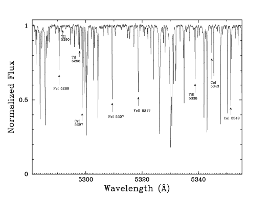
The data were extracted and wavelength calibrated with the makee package developed by T. Barlow specifically for HIRES observations. The algorithm performs an optimal extraction using the observed star to trace the profile, and it solves for a wavelength calibration solution by cross-correlating the extracted ThAr spectra with an extensive database compiled by Dr. Barlow. The pairs of exposures were rebinned to the same wavelength scale and coadded conserving flux. Finally, we continuum fit the summed spectra with a routine similar to IRAF, using the Arcturus spectrum (Griffin, 1968) as a guide in the bluest orders where the flux rarely recovers to the continuum. An example of a typical spectral order is presented in Figure 1 and we identify several representative absorption line features.

The sample of stars were kinematically selected from the study of Carney et al. (1994) to be members of the thick disk according to the following criteria. Our large initial list excluded stars with any uncertain observational parameters, known subgiants, stars whose reddenings might exceed 0.05 mag, and all stars known to be multiple-lined or double-lined. To avoid stars whose lifetimes are shorter than the age of the thick disk, we avoided stars with the “TO” flag (meaning their colors place them near the main sequence turn-off for globular clusters of similar metallicity). We further restricted the list to stars with

$-$1.1 $\leq$ [M/H] $\leq-0.4$ to probe the thick disk metallicity regime, and likewise eliminated stars whose orbits did not carry them farther than 600 pc from the plane. To further maximize the probability of observing thick disk stars within this sample, we restricted the $\tilde{V}$ velocities to lie between $-20$ and $-100$ km s^-1 . While these criteria help minimize the contamination of the thick disk sample from metal-rich halo stars and metal-poor thin disk stars, these stellar populations do overlap in both metallicity and kinematic properties and the possibility of contamination exists. In general, the overlap between the thick and thin disk populations is small (as determined from proper motion studies; e.g. Carney et al. 1989) but the problem deserves further observational attention. Table 2 summarizes values of the observed stars’ photometric temperatures, high-resolution and low signal-to-noise spectroscopic metallicity, stellar gravities determined with Hipparcos measurements (ESA, 1997), and stellar kinematics and galactic orbital parameters from Carney et al. (1994). All of the stars are G dwarfs found in the solar neighborhood with distances of $d_{pc}=50-100$ pc. In those cases where there are Hipparcos parallax measurements, we calculated the stellar gravity according to the equations presented in Appendix A. The uncertainties in the parallax and photometry imply an error in $\log(g/g_{\odot})$ of $\approx 0.1$ dex. In the following section, we will compute spectroscopic physical parameters for each star and compare with the photometric values presented here.

3 ABUNDANCE ANALYSIS

In this section we outline the prescription to measure elemental abundances for our sample of thick disk stars. In short, we measured equivalent widths with the package getjob, implement Kurucz model stellar atmospheres, culled $\log gf$ values from the literature, and used the stellar analysis package MOOG to constrain the spectroscopic physical parameters and determine the elemental abundances.

3.1 Equivalent Widths

We first compiled a list of nearly 1000 reasonably unblended lines from the solar spectrum (Moore et al., 1966) and an extensive literature search. The equivalent width, $W_{\lambda}$, for each line was then measured with the getjob package developed by A. McWilliam for stellar spectroscopic analysis (McWilliam et al., 1995a). In the majority of cases, we fit the absorption lines with single Gaussian profiles which provide an excellent match to the majority of observations. When necessary we fit regions with multiple Gaussians or calculated an integrated equivalent width using Simpson’s Rule. The latter approach was particularly important for strong Ca I and Mg I lines. The getjob program yields an error estimate for each $W_{\lambda}$ value based on the goodness-of-fit and signal-to-noise of the spectra. The typical $1\sigma$ error for a single component fit is $\approx 2$ mÅ. With the exception of a few special cases, those lines with errors exceeding $20\%$ were eliminated from the subsequent abundance analysis. We also focused on unsaturated lines, specifically lines with $W_{\lambda}/\lambda<(100{\rm m\AA})/(5000{\rm\AA})$. Table 3 lists the $W_{\lambda}$ values for the measured absorption lines. We have flagged those absorption lines which we believe are blended or have incorrect $gf$ values.

Table 3: EW MEASUREMENTS

Ion	$\lambda$	EP	log $gf$	Ref	Sun	G66-51	G84-37	G88-13	G92-19	G97-45	G114-19	G144-52	G181-46	G211-5	G247-32
	(Å)	(eV)			(mÅ)	(mÅ)	(mÅ)	(mÅ)	(mÅ)	(mÅ)	(mÅ)	(mÅ)	(mÅ)	(mÅ)	(mÅ)
O I	7771.954	9.140	$0.360$	62	71.5	20.4	48.6	30.3	42.6	60.7	36.5	50.5	39.8	33.3	46.0
O I	7774.177	9.140	$0.210$	62	63.7	17.2	37.6	23.0	35.7	52.8	32.8	41.8	33.8		44.2
O I	7775.395	9.140	$-0.010$	62	53.2	11.8	26.8	17.0	26.0	42.5	23.2		27.9	21.2	34.3
Na I	5682.647	2.100	$-0.890$	99	90.0	51.1	22.6	108.4	66.2	93.4	87.5	74.0		91.1	89.0
Na I	5688.210	2.100	$-0.580$	99	119.1	72.5	37.2	$>$120	86.1	113.2		95.5	102.8	115.2	115.0

3.2 Model Stellar Atmospheres

Throughout the abundance analysis we adopt Kurucz stellar atmospheres (Kurucz, 1988) with convection on and 72 layers with optical depth steps, $\Delta\tau=0.125$, ending at $\tau=100$. Depending on the application, we either interpolated between the stellar atmosphere grids kindly provided by R. Kurucz or implemented the Kurucz package atlas9 to calculate specific models. The former approach has the advantage that the interpolation can be performed with minimal human intervention and at minimal computational cost. In particular, we relied upon the grids to narrow in on the spectroscopic physical parameters of each star ($\S$ 3.4). When applicable we constructed model atmospheres with enhanced $\alpha$-elements using the $+0.4$ dex enhanced Rosseland opacities and the appropriate opacity distribution functions.

3.3 $gf$ Values

Columns 4 and 5 of Table 3 list the adopted $gf$ values and their references for our sample of measured absorption lines. In general, we selected the most accurate and recent laboratory measurements available, avoiding solar $gf$ values where possible. Even with these accurate laboratory values, however, the $gf$ values pose a major source of uncertainty in the analysis particularly with respect to obtaining measurements relative to the solar meteoritic abundances which will serve as our abundance reference frame. We address this issue in $\S$ 4 by performing an analysis of the solar spectrum. In the following, we discuss the criteria established to select the Fe I and Fe II $gf$ values which are critical in determining the spectroscopic atmospheric parameters of each star. We reserve comments on the remaining elements to $\S$ 5.

Figure 2: Plots of ${\epsilon({\rm Fe})}$ values versus Excitation Potential (EP) for six different sets of Fe I $gf$ values: (a) all samples with the priority given in the text, (b) Hannover measurements, (c) Oxford measurements, (d) O’Brian values, and (e) May74+GK81. The various data sets yield systematically different ${\epsilon({\rm Fe})}$ results. In particular, note the offset between the Hannover and May74+GK81 values which cover nearly the same range in EP space. In our analysis, we have chosen to discount the May74+GK81 $gf$ measurements.

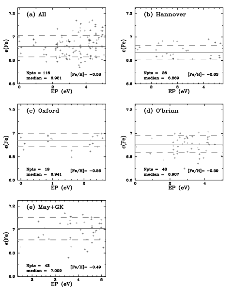
To minimize the uncertainties and systematic errors associated with solar $gf$ values, we restricted the Fe I analysis to laboratory $gf$ measurements. The principal sources that we considered are: (1) the Hannover measurements (Bard et al., 1991; Bard & Kock, 1994), (2) the Oxford $gf$ values (Blackwell et al., 1995a), (3) the O’Brian values (O’Brian et al., 1991), and (4) the May74+GK81 sample (May et al., 1974; Gurtovenko & Kostik, 1981). At present, these are the most accurate measurements for a sizeable number of Fe I lines in our wavelength range. To investigate systematics associated with the various Fe I $gf$ data sets, we performed a thorough Fe abundance analysis of the star G114$-$19. In the process, we identified several lines that yielded highly discrepant ${\epsilon({\rm Fe})}$ values even though there was no obvious blend. These lines are flagged in Table 3 and were removed from any subsequent analysis. In Figure 2 we present the ${\epsilon({\rm FeI})}$ values versus excitation potential (EP) for the four sets of Fe I $gf$ values as well as the entire Fe I $gf$ sample for the G114$-$19 star assuming a Kurucz model atmosphere with $T_{eff}=5310$K, $\log g=4.57$, [M/H] $=-0.60$, and $\xi=0.80{\rm\;km\;s^{-1}}$. Panel (a) presents the complete sample of lines where for lines with multiple $\log gf$ measurements we prioritized the values in this order: Hannover, Oxford, O’Brian, and May74+GK81. The remaining panels present the $gf$ subsets for the (b) Hannover (c) Oxford, (d) O’Brian, and (e) May74+GK81 sources. We observe the following trends. First, the Oxford set of lines which all have EP $<2.5$ eV yield systematically higher ${\epsilon({\rm Fe})}$ values than the Hannover group whose typical EP $>2$ eV. The discrepancy in ${\epsilon({\rm Fe})}$ derived from these two $gf$ data sets has been discussed at length in the literature (Blackwell et al., 1995b; Holweger et al., 1995). Both groups are confident in the accuracy of their laboratory measurements and have argued that the other’s solar equivalent width measurements or spectral analysis techniques are to blame. The fact that this offset is also apparent in our solar-like stars favors the assertion put forth by Grevesse & Sauval (1999) that this EP dependent disagreement indicates an error in the model atmospheres. Grevesse & Sauval (1999) suggest an ad hoc modification to the solar atmosphere $T-\tau$ relation which could be applied to our sample of stars but is beyond the scope of the paper. Instead we chose to adopt the Hannover and Oxford $gf$ values with the caveat that the observed offset could result in an underestimate of the true effective temperature. As described in $\S$ 4, we derive a $T_{eff}$ value for the Sun based on these $gf$ values and the Kurucz atmospheres which is in good agreement with the known value. Furthermore, we perform an abundance analysis relative to a solar analysis with the same model atmospheres and stellar abundance techniques which should minimize any of the systematic effects that the Grevesse & Sauval (1999) atmosphere addresses. Contrary to the Oxford/Hannover discrepancy, the O’Brian lines (Panel d) cover a larger range of EP and yield ${\epsilon({\rm Fe})}$ values with a median in between the Oxford and Hannover groups. Furthermore, the few lines with EP $<2$ eV do not show systematically higher ${\epsilon({\rm Fe})}$ values, although this could be the result of small number statistics or inaccuracies in the O’Brian $gf$ values. In any case, we include this large sample of reasonably accurate values which comprise almost $50\%$ of our total Fe I line-list. Finally, consider the May74+GK81 lines. These lines cover nearly the same EP range as the Hannover data set yet yield even higher ${\epsilon({\rm Fe})}$ values than the Oxford sample. Given the greater accuracy of the Hannover measurements, we have decided to discount the May74+GK81 sample altogether.

In contrast to the Fe I lines, there are few accurate Fe II $gf$ measurements and a careful intracomparison is not warranted. The lack of Fe II $gf$ values is particularly unfortunate because Fe⁺ is the dominant ionization state of Fe in these thick disk stars and therefore the Fe II measurements are less sensitive to non-LTE conditions or model atmosphere inaccuracies. All of the adopted Fe II $gf$ values are laboratory measurements taken from the following sources listed in decreasing priority: Schnabel et al. (1999); Bi$\rm\acute{e}$mont et al. (1991); Heise & Kock (1990); McWilliam et al. (1995b); Kroll & Kock (1987); Moity (1983); Fuhr et al. (1988).

Figure 3: Plots of ${\epsilon({\rm Fe})}$ vs. the reduced equivalent width ($\log W_{\lambda}/\lambda$) and Excitation Potential (EP) derived from the Fe I lines for the 10 program stars. The ${\epsilon({\rm FeI})}$ values correspond to standard model atmospheres with physical parameters listed in Table 4. These parameters were determined by minimizing the trends of ${\epsilon({\rm Fe})}$ vs. $\log W_{\lambda}/\lambda$ and EP simultaneously and by requiring that the median ${\epsilon({\rm Fe})}$ value from Fe I match that for Fe II.

3.4 Spectroscopic Atmospheric Parameters

We now proceed to determine the spectroscopic atmospheric parameters – temperature $T_{eff}$, gravity $\log g_{spec}$, microturbulence $\xi$, and metallicity [Fe/H] – for each star. Following standard practice, we assume local thermodynamic equilibrium (LTE) holds throughout the stellar atmosphere which is a good assumption for G dwarf stars. To perform the analysis, we have used the stellar line analysis software package MOOG (v. 1997) kindly provided by C. Sneden. In the mode abfind, the MOOG package inputs a model stellar atmosphere, and a list of data on each absorption line ($W_{\lambda}$, $\lambda$, EP, $\log gf$) and then matches the observed $W_{\lambda}$ values with a computed $W_{\lambda}$ value by adjusting the elemental abundance. For damping, we assumed the Unsold approximation with no enhancement. As a check, we experimented with other assumptions for the damping, in particular the Blackwell correction and a factor of two enhancement to the Unsold approximation. To our surprise, under neither of these latter assumptions were we able to derive a model atmosphere which was physically reasonable. Specifically, the enhancements suggest a lower microturbulence which in turn require a lower temperature which then implies a lower microturbulence. In any case, we have adopted the same damping approximation (no enhancement) for our solar analysis ($\S$ 4) and hope to have minimized the effects on our final results.

To measure the spectroscopic atmospheric parameters, one modifies the model atmosphere to satisfy three constraints: (1) minimize the slope of ${\epsilon({\rm FeI})}$ vs. $W_{\lambda}/\lambda$; (2) minimize the slope of ${\epsilon({\rm FeI})}$ vs. EP; and (3) require that the median ${\epsilon({\rm FeI})}$ value equal the median ${\epsilon({\rm FeII})}$ value. The first constraint determines $\xi$ because the adopted microturbulence value has a significant effect on the abundances derived from large equivalent width lines, i.e. lines which suffer from saturation. Therefore, requiring that the ${\epsilon({\rm FeI})}$ values exhibit no trend with $W_{\lambda}$ sets the microturbulence of the model atmosphere. Similarly, the slope of ${\epsilon({\rm FeI})}$ values vs. EP is sensitive to the effective temperature because the predicted population of various EP levels is a function of the temperature of the stellar atmosphere. Finally, $\log g$ is constrained by requiring that the Fe abundance derived from the Fe II lines – which are sensitive to $\log g$ – match the Fe abundance from Fe I. This parameter is perhaps the most uncertain as it is dependent on systematic errors in both the Fe I and Fe II $gf$ values. In practice, the constraints are mildly degenerate in the atmospheric parameters and one iteratively solves for the model atmosphere. Our approach was to guess values of $\log g$ and [Fe/H] and then use a $\chi^{2}$ minimization routine auto_ab4 developed by A. McWilliam to find the $\xi$ and $T_{eff}$ values which minimize the slope of ${\epsilon({\rm FeI})}$ vs. $\log W_{\lambda}/\lambda$ and EP. This notion placed typical error estimates for $T_{eff}$ and $\xi$ at $\approx 50$ K and 0.05 km s^-1 respectively. We then adjusted the $\log g$ and [Fe/H] values and reran auto_ab4 until Fe I and Fe II were brought into agreement with one another. To minimize our effort, we calculated the stellar atmospheric models by interpolating the grids provided on R. Kurucz’s web site. Once we determined reasonable values for $T_{eff}$, $\log g$, $\xi$, and [Fe/H], we derived a final stellar atmosphere with atlas9. This final model atmosphere was then adopted in the abundance analysis of all of the elements. As we shall see, nearly every star observed in this sample has enhanced $\alpha$-elements (Mg, Si, O, etc.). For the stars with [Fe/H] $\approx-0.5$, Mg is a principal source of electrons and therefore an $\alpha$-enhancement can significantly modify the model atmosphere. In particular, ignoring the higher electron density associated with an enhanced magnesium abundance leads to a systematic overestimate of the stellar gravity. Therefore, we also derived an $\alpha$-enhanced model atmosphere with atlas9 (assuming [$\alpha$/Fe]=+0.4 dex and using the appropriate opacities) and performed a complete abundance analysis with this enhanced atmosphere including a reanalysis of the atmospheric parameters. We have found, however, that these atmospheres imply small differences from the results of the standard atmospheres.

Table 4: ATMOSPHERIC SPECTROSCOPIC PARAMETERS

Star	$T_{spec}$	[M/H]	$\log g$	$\xi$		$T_{spec}^{\alpha}$	[M/H]α	$\log g^{\alpha}$	$\xi^{\alpha}$
	(K)			(km/s)		(K)			(km/s)
G66-51	5220	$-1.00$	4.55	0.64		5255	$-1.00$	4.48	0.90
G84-37	5700	$-1.20$	4.20	1.11		5765	$-1.20$	4.15	1.20
G88-13	5220	$-0.40$	4.60	0.86		5270	$-0.30$	4.55	1.05
G92-19	5530	$-0.60$	4.45	1.05		5545	$-0.60$	4.40	1.15
G97-45	5550	$-0.45$	4.50	0.90		5580	$-0.40$	4.40	1.10
G114-19	5310	$-0.60$	4.57	0.80		5350	$-0.60$	4.52	0.95
G144-52	5575	$-0.55$	4.58	0.90		5610	$-0.55$	4.45	1.13
G181-46	5380	$-0.50$	4.53	0.82		5400	$-0.50$	4.45	0.95
G211-5	5320	$-0.40$	4.55	1.07		5360	$-0.40$	4.45	1.25
G247-32	5360	$-0.40$	4.45	0.88		5400	$-0.40$	4.35	1.05

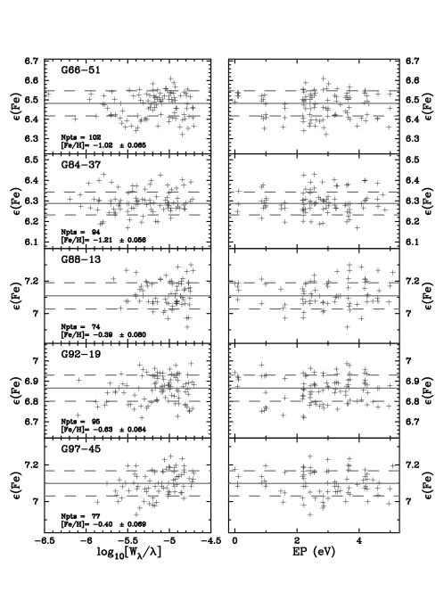
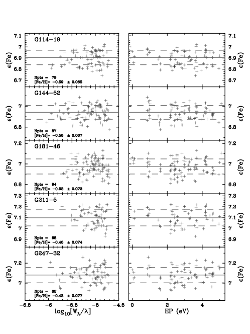
Figure 3 presents (a) ${\epsilon({\rm FeI})}$ vs. $W_{\lambda}/\lambda$ and (b) ${\epsilon({\rm FeI})}$ vs. EP plots for every thick disk star in the sample assuming the standard model atmospheres. The physical parameters of the final model atmospheres (with and without $\alpha$-enhancement) are listed in Table 4. As expected, the $\alpha$-enhanced models tend to have lower $\log g$ values by $\approx 0.05-0.1$ dex. We will show that the typical $\alpha$-enhancement is $0.2-0.3$ dex so the most accurate spectroscopic gravity is more likely the average of the two values. Furthermore, the $\alpha$-enhanced models require slightly higher $T_{eff}$ values to compensate the larger opacity implied by the increase in electron density. With the notable exception of G84-37, our spectroscopic $T_{eff}$, $\log g$, and [Fe/H] values are systematically higher than the photometric values based on the Carney et al. (1994) observations listed in Table 2. Excluding G84-37, the offset between the spectroscopic temperatures and the Carney et al. (1994) values is $<T_{spec}-T_{Carn94}>\;=+87\pm 15$K for the standard atmospheres. On the other hand, comparing the spectroscopic values with the Alonso et al. (1995) color-temperature relations based on the Infrared Flux Method (IRFM), we find excellent agreement: $<T_{spec}-T_{Alonso96}>\;=-1\pm 12$K for the 4 stars with $uvby$ photometry. The agreement is possibly the result of small number statistics, however, particularly given the excellent overall agreement between the two photometric techniques for low mass main sequence stars (Alonso et al., 1996b). As we increase the sample of thick disk stars, it will be important to further compare the various temperature scales. Finally, as we will ultimately be interested in a comparison of the Edvardsson et al. (1993) and Chen et al. (2000) results with our analysis, it is important to examine their temperature scales. As an indirect test, we compared the 33 overlapping stars from the Alonso et al. (1996a) and Edvardsson et al. (1993) samples which are nearby (minimally affected by dust) and in the appropriate temperature range $(T_{eff}<5900$K). We find $<T_{Alonso96}-T_{Edvard}>\;=-95\pm 6$K, so we will assume that our stars are $\approx 100$K cooler than the Edvardsson et al. (1993) temperature scale. Similarly Chen et al. (2000), whose temperatures are based on the IRFM scale, report a systematically lower temperature $(\approx 70$K) than Edvardsson et al. (1993). Therefore, we will assume no temperature offset between our analysis and that of Chen et al. (2000).

While a difference between the spectroscopic and the color-temperature scales may not be surprising, the stellar gravity offset is more difficult to explain. Taking the average spectroscopic gravity from the standard and $\alpha$-enhanced atmospheres (and again ignoring G84-37 for now), the average offset is $<\log g_{Hipp}-\log g_{spec}>\;=-0.08\pm 0.01$ dex. We might suggest that a systematic error in the Fe II $gf$ values has biased the spectroscopic gravity, but our $\log g$ measurement for the Sun is in excellent agreement with the known value. A fraction of the offset (0.03$-$0.05 dex) can be explained by the difference in assumed effective temperature, but it can not account for the entire discrepancy. Nonetheless, the effect of even a 0.1 dex error in $\log g$ has a minimal impact on the abundances we derive, particularly since we rely primarily on the Fe I lines to determine [Fe/H]. Finally, note that the metallicity we compute from the Fe lines is systematically $\approx 0.1$ dex higher than the [M/H] values derived by Carney et al. (1994) from low $S/N$ spectra. In this case, the difference is largely explained by the offset in temperature and gravity as both imply a higher metallicity. While a 0.1 dex systematic error in the spectroscopic metallicity measurements will not significantly affect our conclusions on the abundance trends of the thick disk stars, a systematic error in the Carney et al. (1994) [M/H] measurements could have important implications for the metallicity distribution function of the thick disk. Therefore, we will carefully reassess this discrepancy once we have a larger, statistically significant sample of accurate spectroscopic measurements.

Table 5: ERROR ANALYSIS FOR G84-37

Ion	$N$	$\Delta T_{eff}$	$\Delta T_{eff}$	$\Delta\log g$	$\Delta\log g$	$\Delta\xi$	$\Delta\xi$	$\Delta\left[\,\frac{\rm M}{\rm H}\,\right]$	$\Delta\left[\,\frac{\rm M}{\rm H}\,\right]$	$\alpha$
		+50K	–50K	+0.05	–0.05	+0.05	–0.05	+0.05	–0.05
Fe I/H	94	$+0.050$	$-0.042$	$-0.002$	$+0.006$	$-0.006$	$+0.011$	$+0.000$	$+0.000$	$+0.025$
Fe II/H	17	$-0.003$	$+0.001$	$+0.018$	$-0.017$	$-0.011$	$+0.013$	$+0.006$	$-0.005$	$-0.009$
O I/Fe	3	$-0.102$	$+0.090$	$+0.017$	$-0.023$	$+0.004$	$-0.009$	$-0.003$	$+0.002$	$-0.080$
Na I/Fe	3	$-0.023$	$+0.015$	$-0.002$	$-0.001$	$+0.005$	$-0.010$	$+0.000$	$+0.000$	$-0.011$
Mg I/Fe	5	$-0.037$	$+0.030$	$+0.002$	$-0.006$	$+0.006$	$-0.011$	$+0.001$	$+0.001$	$-0.017$
Si I/Fe	12	$-0.032$	$+0.025$	$+0.004$	$-0.007$	$+0.004$	$-0.008$	$+0.000$	$+0.000$	$-0.018$
S I/Fe	1	$-0.089$	$+0.077$	$+0.017$	$-0.024$	$+0.005$	$-0.011$	$-0.002$	$+0.001$	$-0.067$
Ca I/Fe	17	$-0.017$	$+0.008$	$-0.003$	$+0.000$	$+0.000$	$-0.005$	$+0.000$	$+0.001$	$-0.014$
Sc II/Fe	4	$-0.040$	$+0.031$	$+0.020$	$-0.025$	$+0.003$	$-0.009$	$+0.005$	$-0.006$	$+0.001$
Ti I/Fe	17	$+0.003$	$-0.012$	$+0.002$	$-0.003$	$+0.002$	$-0.005$	$+0.000$	$+0.001$	$+0.000$
Ti II/Fe	16	$-0.038$	$+0.030$	$+0.021$	$-0.024$	$+0.000$	$-0.008$	$+0.006$	$-0.005$	$-0.009$
Cr I/Fe	12	$+0.003$	$-0.004$	$+0.001$	$-0.003$	$+0.003$	$-0.002$	$+0.001$	$+0.000$	$+0.004$
Cr II/Fe	4	$-0.060$	$+0.049$	$+0.020$	$-0.025$	$+0.001$	$-0.007$	$+0.002$	$-0.003$	$-0.037$
Mn I/Fe	10	$-0.013$	$+0.002$	$+0.002$	$-0.006$	$+0.005$	$-0.011$	$+0.000$	$+0.000$	$-0.005$
Co I/Fe	1	$+0.000$	$-0.009$	$+0.003$	$-0.007$	$+0.005$	$-0.011$	$+0.001$	$+0.001$	$+0.009$
Ni I/Fe	21	$-0.021$	$+0.012$	$+0.002$	$-0.006$	$+0.003$	$-0.009$	$+0.000$	$-0.001$	$-0.013$
Cu I/Fe	2	$-0.010$	$+0.002$	$+0.005$	$-0.006$	$+0.006$	$-0.010$	$+0.000$	$+0.000$	$+0.000$
Zn I/Fe	2	$-0.037$	$+0.029$	$+0.010$	$-0.014$	$-0.001$	$-0.004$	$+0.002$	$-0.002$	$-0.022$
Y II/Fe	5	$-0.035$	$+0.027$	$+0.020$	$-0.026$	$-0.002$	$-0.002$	$+0.006$	$-0.006$	$-0.003$
Ba II/Fe	3	$-0.023$	$+0.017$	$+0.013$	$-0.013$	$-0.023$	$+0.024$	$+0.006$	$+0.001$	$-0.002$

Table 6: ERROR ANALYSIS FOR G114-19

Ion	$N$	$\Delta T_{eff}$	$\Delta T_{eff}$	$\Delta\log g$	$\Delta\log g$	$\Delta\xi$	$\Delta\xi$	$\Delta\left[\,\frac{\rm M}{\rm H}\,\right]$	$\Delta\left[\,\frac{\rm M}{\rm H}\,\right]$	$\alpha$
		+50K	–50K	+0.05	–0.05	+0.05	–0.05	+0.05	–0.05
Fe I/H	79	$+0.031$	$-0.042$	$-0.001$	$+0.004$	$-0.007$	$+0.006$	$+0.008$	$-0.007$	$+0.006$
Fe II/H	20	$-0.021$	$+0.019$	$+0.026$	$-0.028$	$-0.005$	$+0.005$	$+0.011$	$-0.012$	$+0.031$
O I/Fe	3	$-0.079$	$+0.084$	$+0.025$	$-0.031$	$+0.006$	$-0.005$	$-0.014$	$+0.011$	$-0.015$
Na I/Fe	3	$+0.002$	$+0.007$	$-0.007$	$+0.005$	$+0.006$	$-0.005$	$-0.006$	$+0.005$	$+0.011$
Mg I/Fe	6	$-0.016$	$+0.025$	$-0.005$	$+0.003$	$+0.007$	$-0.005$	$-0.005$	$+0.004$	$+0.023$
Al I/Fe	1	$-0.001$	$+0.011$	$-0.003$	$+0.001$	$+0.006$	$-0.005$	$-0.007$	$+0.007$	$+0.001$
Si I/Fe	14	$-0.031$	$+0.041$	$+0.005$	$-0.008$	$+0.005$	$-0.004$	$+0.001$	$-0.002$	$+0.035$
S I/Fe	1	$-0.068$	$+0.074$	$+0.025$	$-0.030$	$+0.007$	$-0.005$	$-0.012$	$+0.010$	$-0.012$
Ca I/Fe	16	$+0.014$	$-0.003$	$-0.017$	$+0.020$	$+0.000$	$+0.001$	$+0.002$	$+0.001$	$+0.031$
Sc II/Fe	7	$-0.030$	$+0.039$	$+0.023$	$-0.026$	$+0.006$	$-0.002$	$+0.007$	$-0.007$	$+0.049$
Ti I/Fe	41	$+0.030$	$-0.020$	$-0.002$	$+0.002$	$+0.006$	$-0.002$	$-0.006$	$+0.008$	$+0.003$
Ti II/Fe	12	$-0.028$	$+0.038$	$+0.021$	$-0.024$	$-0.003$	$+0.006$	$+0.008$	$-0.007$	$+0.031$
V I/Fe	15	$+0.037$	$-0.028$	$-0.002$	$+0.001$	$+0.006$	$-0.004$	$-0.006$	$+0.007$	$+0.020$
Cr I/Fe	13	$+0.012$	$-0.009$	$-0.015$	$+0.008$	$-0.006$	$+0.000$	$-0.003$	$-0.002$	$+0.001$
Cr II/Fe	5	$-0.044$	$+0.053$	$+0.023$	$-0.027$	$+0.003$	$-0.002$	$+0.000$	$-0.001$	$+0.002$
Mn I/Fe	10	$+0.024$	$-0.027$	$-0.001$	$-0.001$	$+0.005$	$-0.004$	$-0.005$	$+0.005$	$+0.013$
Co I/Fe	9	$+0.003$	$+0.008$	$+0.007$	$-0.010$	$+0.006$	$-0.005$	$-0.002$	$+0.002$	$+0.030$
Ni I/Fe	28	$-0.008$	$+0.014$	$-0.008$	$+0.000$	$-0.003$	$+0.001$	$+0.004$	$-0.005$	$+0.013$
Cu I/Fe	1	$-0.015$	$+0.028$	$+0.008$	$-0.010$	$+0.005$	$-0.003$	$+0.000$	$+0.001$	$+0.021$
Zn I/Fe	2	$-0.031$	$+0.041$	$+0.007$	$-0.010$	$-0.005$	$+0.006$	$+0.005$	$-0.006$	$+0.002$
Y II/Fe	1	$-0.023$	$+0.030$	$+0.016$	$-0.023$	$-0.010$	$+0.007$	$+0.007$	$-0.011$	$+0.000$
Ba II/Fe	2	$-0.016$	$+0.024$	$+0.012$	$-0.016$	$-0.016$	$+0.015$	$+0.011$	$-0.013$	$+0.003$
Eu II/Fe	1	$-0.029$	$+0.039$	$+0.023$	$-0.026$	$+0.006$	$-0.004$	$+0.007$	$-0.008$	$+0.055$

3.5 Error Analysis

To assess the systematic effects of the model atmospheric parameters on the elemental abundance ratios, we have performed a standard abundance error analysis. We calculated the elemental abundances for 10 atmospheric models for two stars (G114-19 and G84-37) using the Kurucz atmosphere grids: (1) the best fit model; (2,3) $T^{\prime}=T\pm 50$K; (4,5) $\xi^{\prime}=\xi\pm 0.05{\rm\;km\;s^{-1}}$; (6,7) $\log g^{\prime}=\log g\pm 0.05$; (8,9) [M/H]^′ = [M/H] $\pm 0.05$ dex; and (10) a +0.4 $\alpha$-enhanced atmosphere. The two stars were chosen to have significantly different stellar atmospheres and the range of parameters roughly corresponds to our estimated $1\sigma$ statistical uncertainty. Tables 5 and 6 summarize the results of the error analysis for the two stars. For those elements with $N>5$ absorption lines, we expect the uncertainties in the abundances to be dominated by errors in the atmospheric parameters. For the remaining elements, the errors in $W_{\lambda}$ (i.e. Poissonian noise, blends, continuum error) are significant. In $\S$ 5 we remark on those elements for which errors in the $W_{\lambda}$ measurements are a particular problem.

3.6 Hyperfine Splitting

Isotopes with an odd number of protons and/or neutrons experience hyperfine interactions between the nucleus and electrons. These interactions split the lines into multiple components with typical separations of $1-10$mÅ. For strong lines with large equivalent width the effect is to de-saturate the absorption line, a phenomenon which must be taken into account in order to accurately measure the elemental abundance. In the case of several Cu I lines, for example, hyperfine splitting leads to a correction of over 0.5 dex. For our abundance analysis, we have included hfs corrections for Mn, Ba, Sc, Co, and Cu. With the exception of Ba where we have implemented the results from McWilliam (1998), we adopt the wavelengths of the hfs transitions from Kurucz’s hyperfine tables (Kurucz, 1999) and calculated the relative $gf$ strengths according to the equations in Appendix B. Table 11 lists all of the hfs transitions considered here. For these lines we implemented the MOOG package in the synthesis mode blends which matches the observed equivalent widths to that calculated from a synthesis of the blended hyperfine lines.

Figure 4: ${\epsilon({\rm Fe})}$ values vs. $\log W_{\lambda}/\lambda$ and EP derived from 112 Fe I measured in the Kurucz solar spectrum. By minimizing the slope of ${\epsilon({\rm Fe})}$ with $\log W_{\lambda}/\lambda$ and EP, we derived the ’best’ atmospheric parameters for the Sun ($T_{eff}$, $\log g$, [M/H], $\xi$). To our surprise, these parameters agree very well with the known parameters.

4 SOLAR ANALYSIS

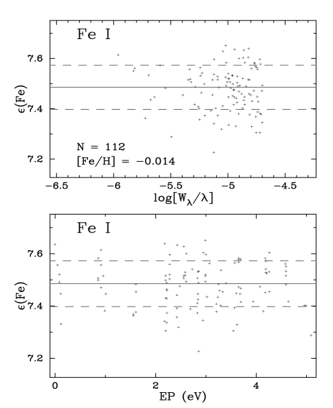
In order to facilitate abundance comparisons between our thick disk sample and other stellar populations or galactic systems (e.g. the damped Ly$\alpha$ systems), it is crucial to compare our results with a spectroscopic solar analysis. In this fashion, we can report our abundances relative to the solar meteoritic abundances (Grevesse et al., 1996) by comparing the solar analysis with the meteoritic values. This exercise also accentuates systematic errors associated with the $\log gf$ values or blending of individual ions. More ambitiously, by making a line by line comparison we might eliminate errors in the model atmospheres, damping, and the stellar analysis package, particularly given that these thick disk stars have similar spectral types to the Sun. Therefore, we performed an elemental abundance analysis of the Sun applying the exact same techniques utilized for the thick disk stars. The equivalent widths were measured with the getjob package, we adopted Kurucz model atmospheres, and constrained the atmospheric parameters with auto_ab4. The only differences lie in the solar spectrum itself; we have analyzed the Kurucz solar spectrum (Kurucz et al., 1984) obtained with resolving power 522,000 and signal-to-noise in excess of 2000. Column 6 of Table 3 lists the $W_{\lambda}$ measurements for the Sun which were included in the abundance analysis. We estimate that the typical error of each measurement is $1-2$mÅ, the dominant sources of error being line blends and poor continuum determination. Figure 4 presents the ${\epsilon({\rm Fe})}$ vs. $W_{\lambda}/\lambda$ and EP plots for 112 Fe I lines measured from the solar spectrum. Somewhat to our surprise, the physical parameters that we derive are in excellent agreement with the known values: $T_{eff}=5750\pm 50$ K, $\log g=4.44\pm 0.03$, $\xi=1.00\pm 0.03{\rm\;km\;s^{-1}}$, and [M/H] = 0.0 dex. Perhaps most astonishing, the Fe abundance matches the meteoritic value to within 0.015 dex. While the nearly exact agreement is probably fortuitous, our analysis indicates no significant disagreement between the photometric and meteoritic solar Fe abundance.

Table 7: SOLAR ABUNDANCES RELATIVE TO METEORITIC

Ion	${\epsilon({\rm X})}\tablenotemark{a}$	$N$	[X/H]d	[X/H]n	$\sigma$
C I	8.55	4	$0.23$	$0.19$	0.18
O I	8.87	3	$0.12$	$0.12$	0.02
Na I	6.32	3	$0.00$	$-0.01$	0.02
Mg I	7.58	3	$0.03$	$0.04$	0.02
Al I	6.49	2	$-0.09$	$-0.09$	0.05
Si I	7.56	16	$0.00$	$0.01$	0.04
S I	7.20	2	$0.35$	$0.35$	0.00
Ca I	6.35	20	$-0.07$	$-0.05$	0.10
Sc II	3.10	9	$0.17$	$0.17$	0.08
Ti I	4.94	47	$-0.05$	$-0.04$	0.07
Ti II	4.94	19	$0.11$	$0.14$	0.13
V I	4.02	17	$-0.12$	$-0.12$	0.06
Cr I	5.67	14	$0.01$	$0.02$	0.07
Cr II	5.67	6	$0.09$	$0.14$	0.12
Mn I	5.53	9	$-0.21$	$-0.20$	0.07
Fe I	7.50	112	$-0.01$	$-0.02$	0.09
Fe II	7.50	33	$0.00$	$0.01$	0.10
Co I	4.91	10	$0.03$	$0.03$	0.11
Ni I	6.25	33	$0.00$	$-0.01$	0.10
Cu I	4.29	3	$-0.01$	$-0.05$	0.08
Zn I	4.67	2	$0.00$	$0.00$	0.06
Y II	2.23	3	$0.02$	$0.01$	0.02
Ba II	2.22	2	$0.11$	$0.11$	0.12
Eu II	0.54	1	$0.10$	$0.10$

With the atmospheric parameters determined, we constructed a final model atmosphere with atlas9 and measured the elemental abundances of the remaining absorption lines. Table 7 lists the ion, the number of absorption lines analyzed, the median and mean abundance relative to the meteoritic value, and the standard deviation of these measurements. While the majority of ions are consistent with the meteoritic values, there are notable exceptions: Ti II (+0.11 dex), S I (+0.35 dex), C I (+0.23 dex), Mn I ($-$0.21 dex), Cu I ($-$0.13 dex), Cr II (+0.09 dex), and Sc II (+0.19 dex). In each of these cases, either the absolute scale of the $gf$ values is poorly determined or the abundances are very sensitive to the model atmospheres. For example, the S I measurement is based on a single line with very high EP and an uncertain solar $gf$ value from the lunar analysis by Francois (1988). Therefore, we expect the differences between the photometric and meteoritic abundance are entirely due to systematic errors in the $gf$ measurements or errors in the details of the solar model atmosphere. We also considered a solar analysis with the Holweger-M$\ddot{\rm u}$ller solar atmosphere (Holweger & M$\ddot{\rm u}$uller, 1974) with $\xi=1.15{\rm\;km\;s^{-1}}$ as is commonly adopted in stellar abundance studies. With the exception of vanadium, all of the derived abundances are within 0.1 dex of the values listed in Table 7. There is a noticeable increase in ${\epsilon({\rm Fe})}$ derived from the Fe I lines of +0.07 dex which would tend toward slightly higher solar-corrected $\alpha$/Fe values, but by less than +0.05 in most cases.

In order to report abundances relative to the solar meteoritic values, we must apply any offsets between the solar photospheric values we derived and the meteoritic values. The zeroth order correction is to modify our final results by the median value computed for each element as listed in Table 7. With the exception of a few elements, these median corrections are robust and should allow for a reasonable estimate of the absolute abundance. Another approach is to measure a correction for every measured solar absorption line, $\delta\equiv{\epsilon({\rm X})}_{obs}-{\epsilon({\rm X})}_{meteor}$, and subtract this offset from the abundances calculated for each line in the program stars. This is akin to adopting solar $gf$ values. It has the advantage that the results are nearly independent of errors in the $gf$ values and that systematic errors in the model atmospheres and stellar analysis package are minimized. Unfortunately, there are two significant drawbacks: (1) the error in our solar equivalent width measurements are comparable to the expected error in the $gf$ values, and (2) saturated or blended solar lines are excluded limiting one to a smaller sample of absorption lines. In fact, for Fe I this approach tends to increase the scatter in the ${\epsilon({\rm Fe})}$ values. Nevertheless, we will consider this line-by-line solar correction with all of our stars.

5 ELEMENTAL ABUNDANCES

We have computed the elemental abundances for each absorption line with three different approaches (i) standard model atmospheres, (ii) $\alpha$-enhanced model atmospheres, and (iii) standard model atmospheres corrected by the solar abundance analysis to the solar meteoritic abundances as performed in the previous section. Tables 8-17 present [X/Fe], the logarithmic abundances of ion X relative to Fe normalized to solar meteoritic abundances (Grevesse et al., 1996), for the 10 thick disk stars comprising our current sample. Column 2 indicates the number of absorption lines analyzed with the standard and $\alpha$-enhanced atmospheres. Columns 3$-$5 present the median, mean, and standard deviation of the ${\epsilon({\rm X})}$ values for the standard models while columns 6$-$8 present the same quantities for the $\alpha$-enhanced stellar atmospheres. Other than the few exceptions noted below, the $\alpha$-enhanced models have minimal effect on the [X/Fe] ratios. Finally, column 9 lists the number of lines from the solar-corrected analysis and columns 10$-$12 present the corrected mean and median values and the resultant standard deviation.

We turn now to comment on the analysis and results for individual elements. Unless otherwise noted, we consider the median measurements in our discussions and the error bars in the figures refer to the unreduced standard deviation which in the majority of cases are conservative estimates of the true error. In the few cases where the standard deviation is very small $(<0.05$), we plot a minimum error bar of 0.05 dex because we feel this is a lower limit to the statistical error associated with the measurements. We also plot in the upper-right hand corner an estimated systematic error for each abundance measurement derived by adding in quadrature the values listed in Tables 5 and 6. For most of the plots we present the solar-corrected ratios and in a few cases where the corrections are very large we also present the uncorrected values. We also discuss the sensitivity of the results to uncertainties in the atmospheric models, paying particular attention to the possibility that we have overestimated $T_{eff}$ for the majority of stars ($\S$ 3.4). In the following section, we will compare the observed trends of these thick disk stars with the halo (McWilliam et al., 1995b), thin disk (Edvardsson et al., 1993; Chen et al., 2000), and bulge (McWilliam & Rich, 1994) stellar populations.

Table 8: ABUNDANCES FOR G66-51

Table 17: ABUNDANCES FOR G247-32

5.1 Iron

We computed the [Fe/H] values for the program stars from the Fe I and Fe II measurements under the constraint that the adopted stellar gravity gives a median ${\epsilon({\rm Fe})}$ value from the Fe II lines within 0.03 dex of the median ${\epsilon({\rm Fe})}$ value from the Fe I lines. In this section and all further analysis, we take [Fe/H] from the median ${\epsilon({\rm Fe})}$ value of the Fe I lines. While significant uncertainties exist for the Fe I and Fe II $gf$ values, the excellent agreement between our solar spectroscopic Fe abundance and the meteoritic abundance raises our confidence in the absolute value of our [Fe/H] measurements. Furthermore, with the exception of one star, the [Fe/H] values are essentially independent of $\alpha$-enhancement. This one exception, G88-13, has the highest metallicity of all of our program stars but is otherwise unpeculiar. While the difference in [Fe/H] is significant for this star, the majority of elemental abundances relative to Fe are insensitive to the $\alpha$-enhancement and we will generally not include this approach in our discussion.

5.2 Alpha Elements – O, Mg, Si, S, Ca, Ti

Our observations include measurements on a number of $\alpha$-elements. In this subsection, we describe the results. We have grouped the elements into two subsets, one with relatively robust results and the other with poorly constrained measurements.

5.2.1 Silicon, Calcium, Titanium

For the abundances of Si, Ca, and Ti, we have measured over 15 absorption lines and have reasonably accurate laboratory $gf$ values. In the case of silicon, we have adopted the $gf$ values from Garz (1973) adjusted by $+0.1$ dex as recommended by Becker et al. (1980) as well as the solar $gf$ values from Fry & Carney (1997) and McWilliam & Rich (1994) which give ${\epsilon({\rm Si})}$ values in good agreement with the adjusted Garz (1973) abundances. For calcium, we rely solely on the laboratory measurements by Smith & Raggett (1981) while the titanium $gf$ values were gleaned from a number of sources with the Oxford measurements given highest priority.

Figure 5: Solar-corrected [Si/Fe] abundance ratios vs. [Fe/H] metallicity for the 10 thick disk stars. The observations show a clear enhancement and hint at a trend for increasing [Si/Fe] with decreasing [Fe/H]. The dashed line at [Si/Fe] = 0 indicates the solar meteoritic Si/Fe ratio and the gray error bars reflect the $1\sigma$ systematic error from the atmospheric uncertainties.

Silicon is a prototypical $\alpha$-element. In addition to exhibiting an enhancement in metal-poor stars (McWilliam, 1997), theoretically it is expected to be synthesized predominantly in moderate mass $(\approx 20M_{\odot}$) Type II SN (Woosley & Weaver, 1995). In Figure 5, we plot the solar-corrected silicon abundances vs. [Fe/H] for the thick disk stars. The majority are significantly enhanced and there is an indication of higher [Si/Fe] at lower metallicity as found in most metal-poor stellar abundance studies. In terms of the uncertainty in the atmospheric parameters, a decrease in $T_{eff}$ of 100K would further enhance the Si/Fe ratio by 0.06$-$0.08 dex and the ratio is largely insensitive to the other parameters. As discussed in the following section, we contend that the majority of stars are even more enhanced than their thin disk counterparts at the same metallicity. The obvious exceptions are the two highest metallicity stars (G88-13, G211-5) which exhibit relatively low [Si/Fe] values. We shall note, however, that these two stars also show lower values of calcium and oxygen yet significantly enhanced Ti and Mg. These trends might be indicative of an overestimate of temperature for these two stars because Si, Ca, and O are most sensitive to $T_{eff}$ in G dwarf stars.

Figure 6: Solar-corrected [Ca/Fe] abundance ratios vs. [Fe/H] metallicity for the 10 thick disk stars. The observations show a clear enhancement and hint at a trend for increasing [Ca/Fe] with decreasing [Fe/H]. The dashed line at [Ca/Fe] = 0 indicates the solar meteoritic Ca/Fe ratio.

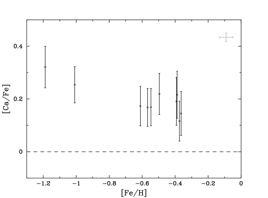
Like silicon, Ca is enhanced in metal-poor stars (McWilliam, 1997) and is predicted to be produced in intermediate mass Type II SN along with silicon (Woosley & Weaver, 1995). Not surprisingly, then, the abundance trends that we observe for silicon are well matched by calcium. Figure 6 presents the solar-corrected Ca abundances relative to Fe vs. [Fe/H]. All of the stars exhibit enhanced Ca and, similar to Si, there is a mild trend to higher [Ca/Fe] at lower [Fe/H]. Also similar to the silicon results, the two highest metallicity stars show somewhat lower [Ca/Fe]. In contrast to most of the other well measured elements, the Ca measurements for a given star exhibit a fairly large scatter. We expect this is due to a greater uncertainty in the equivalent width measurements for the Ca I lines which often have significant damping wings.

Figure 7: Solar-corrected [Ti/Fe] abundance ratios vs. [Fe/H] metallicity for the 10 thick disk stars. The observations show a clear enhancement yet no trend with metallicity. The dashed line at [Ti/Fe] = 0 indicates the solar meteoritic Ti/Fe ratio.

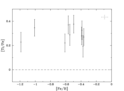
Titanium is traditionally referred to as an $\alpha$-element because it exhibits enhanced abundances in metal-poor stars (Gratton & Sneden, 1991), but it is unclear if the nucleosynthesis of Ti is related to the other $\alpha$-elements (Woosley & Weaver, 1995). Therefore, it would not be surprising if the Ti abundances differ from the results for Si and Ca. In almost every star (G114-19 is an exception), the ${\epsilon({\rm Ti})}$ abundance derived from Ti II exceeds that from Ti I by $\approx 0.10-0.15$ dex. This offset has been discussed in the literature (e.g. Luck & Bond 1985) and has been attributed to non-LTE effects and other possible systematic errors. We find a similar offset in our solar analysis such that the solar-corrected ${\epsilon({\rm Ti})}$ values from Ti I and Ti II abundances are in good agreement for the majority of stars. Because the Ti I results are statistically more robust, we restrict our further analysis to the Ti I results. In Figure 7 we present the solar-corrected [Ti/Fe] measurements as a function of metallicity for the 10 thick disk stars. All of the observations are consistent with a single-valued enhancement, $<[{\rm Ti/Fe}]>=0.29\pm 0.02$, and there is no indication of a trend with metallicity. The latter observation contradicts the general picture described by Si and Ca.

5.2.2 Oxygen, Magnesium, Sulfur

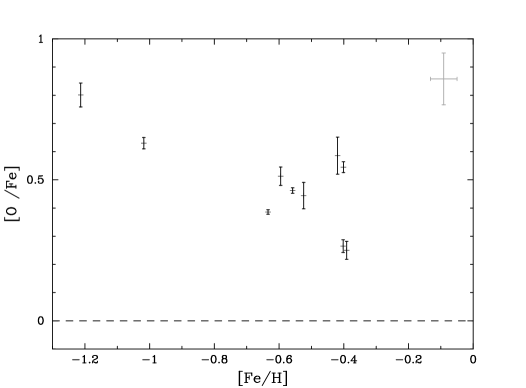
For our choice of observational setup the forbidden O I $\lambda 6300$ line lies within the inter-order gaps of HIRES. Therefore, we rely on the triplet of O I lines at $\lambda\approx 7775$ Å , which have very high excitation potential and are very sensitive to the effective temperature (Tables 5 and 6) and non-LTE effects. We account for CO, CH, and OH molecule formation in deriving our final oxygen abundances which leads to an enhancement of $\approx+0.025$ dex over the abundance derived without molecules. For the Sun, adopting the laboratory $gf$ values from Beveridge & Sneden (1994) and Butler & Zeippen (1991) we find a median ${\epsilon({\rm O})}$ value of [O/H] = $+0.10$ dex with very small scatter. Given the large uncertainty associated with using the O I triplet for an oxygen abundance analysis, the agreement between our solar analysis and the meteoritic value is surprisingly good. Figure 8 plots the [O/Fe] values for the thick disk stars against the stellar metallicity without the solar-correction. We do not apply the solar-correction here because we believe the uncertainty in the solar measurement from the O I triplet is at least as large as 0.1 dex and therefore we would be more likely to introduce an error in the final abundances. The error bars reflect the scatter in the individual measurements for each star which in each case is significantly smaller than the uncertainties from the atmospheric parameters. In particular, even a 50K error in $T_{eff}$ results in nearly a 0.1 dex uncertainty in [O/Fe]. We point out, however, that with the exception of the most metal-poor star, the spectroscopic $T_{eff}$ values are at least as high as the photometric values, implying if anything that we have underestimated the [O/Fe] ratios. Examining the figure, one notes that the majority of stars exhibit enhanced [O/Fe] abundances with tentative evidence for an increasing oxygen abundance at lower metallicity. The two stars with the highest metallicity, however, have nearly solar oxygen abundance. It will be imperative in the future for us to improve on the oxygen measurements, either through the forbidden O I [6300] line or perhaps the near-IR OH lines.

Figure 8: Standard (uncorrected) [O/Fe] abundance ratios vs. [Fe/H] metallicity for the 10 thick disk stars. The observations show a clear enhancement and a likely trend with metallicity. Note the error bars only reflect the scatter in the ${\epsilon({\rm O})}$ values derived from the three O I lines at $\lambda\approx 7775$Å for which the systematic uncertainties are very significant $(>0.1$ dex). The dashed line at [O/Fe] = 0 indicates the solar meteoritic O/Fe ratio.

Figure 9: Standard (uncorrected) [Mg/Fe] abundance ratios vs. [Fe/H] metallicity for the 10 thick disk stars. The observations show a clear enhancement and no trend with metallicity. The dashed line at [Mg/Fe] = 0 indicates the solar meteoritic Mg/Fe ratio.

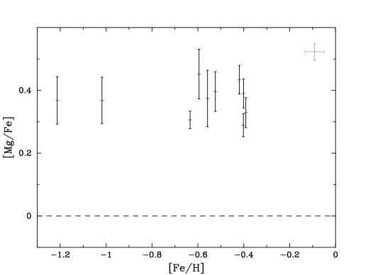
As noted in $\S$ 3.4, measurements of magnesium are particularly important because Mg is a significant contributor of electrons in the stellar atmospheres of our stars. Unfortunately, there are very few Mg I lines with reported $gf$ values that we do not find saturated. Therefore, we are compelled to include a few lines with solar $gf$ values taken from the literature (Edvardsson et al., 1993; McWilliam et al., 1995b). In general, we find good agreement between the various lines and have reasonable confidence in our results. Figure 9 plots the [Mg/Fe] values versus [Fe/H] for the 10 program stars. We observe enhanced Mg in every case, $<[{\rm Mg/Fe}]>=+0.37\pm.02$, with no suggestion of a trend with metallicity. It should be noted, however, that the Mg results for the two most metal-poor stars are derived from a different set of Mg I lines than the other stars. Given the uncertainty in the $gf$ values we adopted and the fact that we could not perform a solar analysis it is possible that there is a systematic error in comparing against the two metal-poor stars although there is no evidence of any offset. The Mg/Fe ratio is insensitive to uncertainties in the atmospheric parameters and we believe the observed enhancement is robust aside from possible errors in the $gf$ values. Because Mg is a principal source of electrons in the stellar atmospheres of our stars and we observe an enhancement of Mg/Fe in every case, it is important to consider $\alpha$-enhanced stellar atmospheres as we have done throughout our analysis.

Figure 10: Solar-corrected [S/Fe] abundance ratios vs. [Fe/H] metallicity for 9 of the 10 thick disk stars. For these measurements, the error bars reflect an estimated 0.3 dex uncertainty in the measurements due to the measurement of a single, weak S I line which has a very large EP and therefore a high sensitivity to $T_{eff}$ and non-LTE effects. There is no indication of a significant enhancement and no trend with metallicity. The dashed line at [S/Fe] = 0 indicates the solar meteoritic S/Fe ratio.

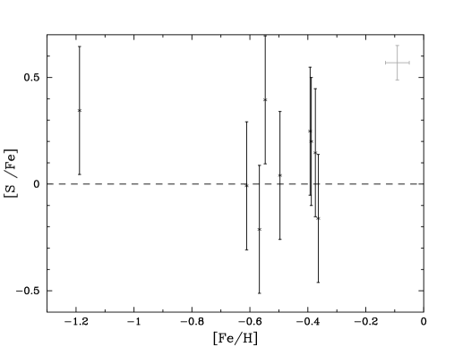
The difficulties associated with sulfur are even more dire than the problems associated with oxygen and magnesium: there is only one useful transition (S I $\lambda 8694$); it lies toward the red end of the spectrum where the sensitivity of HIRES is markedly reduced; it has a high excitation potential with a correspondingly large temperature sensitivity; it is very weak (only 30mÅ in the Sun); and there is no reliable laboratory $gf$ value so a solar analysis is required. We first adopted the $gf$ value from Francois (1988) for the standard and $\alpha$-enhanced values reported in Tables 7$-$17, but our solar analysis shows [S/Fe] $\approx+0.2$ dex indicating a significant correction to the $gf$ value. Figure 10 plots the [S/Fe] abundances for the 9 stars with a measured sulfur equivalent width with the solar-corrected values plotted. In a few cases, we have included $W_{\lambda}$ values less than 10 mÅ. For these stars, the measurement error even exceeds the uncertainties due to errors in the atmospheric parameters. We estimate the total 1$\sigma$ uncertainty to be 0.3 dex and have plotted the error bars accordingly. Given the large errors associated with the [S/Fe] measurements, it is difficult to make any meaningful statements about the sulfur abundance. It is somewhat surprising, however, that the mean ratio $<$[S/Fe]$>\,=0.11\pm 0.08$ is consistent with the solar abundance. Given the importance of sulfur in quasar absorption line studies ($\S$ 6.4), a more careful and extensive stellar abundance analysis of sulfur in metal-poor stars is warranted.

Figure 11: Solar-corrected [Al/Fe] abundance ratios vs. [Fe/H] metallicity for 9 of the 10 thick disk stars. All of the stars show enhanced Al/Fe and there is no trend with metallicity. The dashed line at [Zn/Fe] = 0 indicates the solar meteoritic Zn/Fe ratio.

5.3 Light Elements – Al, Na

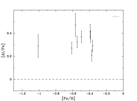
With the exception of the extremely metal-poor stars (Gratton & Sneden, 1988; McWilliam et al., 1995b; Shetrone, 1996), Al is mildly enhanced in metal-poor stars (Tomkin et al., 1985; Edvardsson et al., 1993). As such, Al is sometimes classified as an $\alpha$-element. Contrary to the majority of Al studies, however, Chen et al. (2000) found an enhancement in Al in disk stars with [Fe/H] $\sim 0$ and no enhancement in their metal-poor F and G dwarfs. The Chen et al. (2000) analysis primarily focuses on the pair of Al I lines at 7830Å, while Edvardsson et al. (1993) examined the pair near 8773Å. Unfortunately, all of these transitions fall into the inter-order gasps of our echelle setup. Instead our observations cover three other Al I absorption lines, all with measured laboratory $gf$ values (Buurman et al., 1986): $\lambda=5577,6696,6698$Å. In general, we find good agreement for the Al abundances derived from the two lines at $\lambda\approx 6700$Å, but the $\lambda 5577$ line yields systematically lower values. Unfortunately, this line is too badly blended in the Sun to determine a solar-correction. As such, we have decided to remove the $\lambda 5577$ line from our analysis. For the Sun, the two remaining lines yield a solar Al abundance $\approx 0.1$ dex lower than the meteoritic value therefore we have applied a 0.1 dex offset in the solar-corrected values. In Figure 11 we plot the solar-corrected [Al/Fe] values for the 9 stars where we measured at least one of the lines at $\lambda\approx 6700$Å; the Al I lines are too weak in the most metal-poor star. All of the stars exhibit significant Al enhancements, $<$[Al/Fe]$>=+0.334\pm 0.028$ and there is no trend with metallicity. Our error analysis indicates the Al/Fe ratio is insensitive to the atmospheric parameters; the principal uncertainty lies in the paucity of Al I lines. There is a further systematic error associated with these Al I lines, however. A non-LTE analysis by Baumuller & Gehren (1997) suggests a further enhancement to [Al/Fe] of $\approx 0.15$ dex for stars with metallicity [Fe/H] $\approx-0.5$ dex. We have chosen not to include this non-LTE correction in our analysis, but warn the reader that the reported Al/Fe values may be a lower limit to the true ratio.

Figure 12: Solar-corrected [Na/Fe] abundance ratios vs. [Fe/H] metallicity for the 10 thick disk stars. All of the stars show enhanced Na/Fe and there is a mild trend with metallicity. The dashed line at [Zn/Fe] = 0 indicates the solar meteoritic Zn/Fe ratio.

The observational picture for Na is complicated. The majority of studies on sodium (Tomkin et al., 1985; McWilliam et al., 1995b; Chen et al., 2000) report that Na scales with Fe at all metallicities, although Edvardsson et al. (1993) found a mild Na enhancement at [Fe/H] $\approx-1$ and Pilachowski et al. (1996) report a Na/Fe deficiency in a sample of 60 stars with [Fe/H] $<-1$. Recently, Baumuller et al. (1998) performed a non-LTE analysis of Na and report a trend of decreasing Na with decreasing metallicity. We have measured Na in our thick disk stars based on the observations of four Na I transitions: $\lambda 5682,5688,6154,6160$. None of the $gf$ values are secure for these lines; the latter two are from theoretical work by Lambert & Luck (1978) and we adopt solar $gf$ values for $\lambda 5682,5688$. Therefore, the analysis relative to our solar analysis is essential. Figure 12 presents the solar-corrected [Na/Fe] values versus metallicity for the 10 stars. Every star exhibits mildly enhanced Na with an average $<[{\rm Na/Fe}]>=+0.087\pm 0.014$. The overabundance is statistically significant but the systematic uncertainty (e.g. in the $gf$ values) is on the order of the enhancement. The Na/Fe ratio is remarkably insensitive to the atmospheric parameters therefore the results are probably limited by the small number statistics of measuring only three Na I lines. If we were to apply the results of the non-LTE analysis by Baumuller et al. (1998), it is also possible that the observed Na enhancement would vanish. In summary, we consider the Na/Fe results to be rather poorly constrained yet consistent with no significant departure from the solar abundance.

5.4 Iron-Peak Elements – Sc, V, Cr, Mn, Co, Ni, Cu, Zn

We now turn our attention to the elements with atomic number near Fe, the so-called iron-peak elements. For several of these elements we observe no variations from solar abundance irrespective of the thick disk stellar metallicity. In particular, the relative nickel and chromium abundances show no significant departure from solar abundances for any of the thick disk stars. There is a small offset (+0.03 dex) from solar for the [Ni/Fe] and [Cr/Fe] values in the standard analysis, but we observe a similar difference in the solar analysis such that the corrected abundances are within 0.02 dex of solar for every star but one. The most metal-poor star (G84-37) exhibits a low [Cr/Fe] value which is probably significant and is suggestive of the underabundance observed for Cr in very metal-poor halo stars (e.g. McWilliam et al. 1995). We note in passing that the Cr abundance based on the Cr II absorption lines suggest enhanced [Cr/Fe], typically by $\approx+0.1$ dex. The solar measurements of Cr II, however, exhibit the same enhancement and therefore we propose that the Cr II $gf$ values of Martin et al. (1988) may need to be revised upward by 0.1 dex.

The majority of iron-peak elements, however, exhibit significant departures from the solar ratios and some have clear trends with the stellar metallicity. As these departures offer insights into the nucleosynthetic processes and may distinguish the thick disk stars from other stellar populations, we consider each element in greater detail.

5.4.1 Scandium

Previous studies of scandium have disagreed on the metallicity dependence of [Sc/Fe]. Zhao & Magain (1990) first suggested that Sc was enhanced by $\approx+0.25$ in metal-poor stars based on their analysis of four Sc II lines including several of the lines that we have analyzed. Gratton & Sneden (1991), however, argued that this enhancement was primarily due to inaccuracies in the Sc II $gf$ values. Our solar analysis agrees with this assessment; we find [Sc/H]${}_{\odot}\approx+0.2$ dex using the $gf$ values from Martin et al. (1988) and Lawler & Dakin (1989). Most recently, Nissen et al. (2000) published an analysis of Sc in over 100 G and F dwarf stars with metallicities ranging from [Fe/H] $\approx-1.4-0$. Their study focused on five Sc II lines ($\lambda 5239,5526,5657,6245,6604$) compared against a solar analysis. Their results, based on an hfs analysis from Steffen (1985), indicate an enhancement of [Sc/Fe] with a trend that resembles the $\alpha$-enhancement of metal-poor stars. Compared to our hfs analysis (Table 11), however, the Steffen (1985) compilation overestimates the hfs correction for these Sc II lines, which may account for a significant part if not all of the reported trend (Prochaska & McWilliam, 2000). Figure 13 presents [Sc/Fe] for our full sample as a function of metallicity for the standard (+) and solar-corrected ($\times$) values; the latter reveal a somewhat puzzling picture. While the 8 stars at [Fe/H] $\approx-0.5$ exhibit enhanced scandium, $<$[Sc/Fe]$>=+0.14\pm 0.02$, the most metal-poor stars show only a minor enhancement. This difference could be explained by unidentified blends, but it seems very unlikely given the reasonably close agreement of more than 5 Sc II lines in each star and because it would be difficult to reconcile blends with the solar ${\epsilon({\rm Sc})}$ results. An underestimate of $\approx 150$K in $T_{eff}$ for the stars with [Fe/H] $\approx-0.5$ could explain the observed enhancement, but this too is unlikely given the fact that the spectroscopic $T_{eff}$ values are already $\approx$100K higher than the Carney et al. (1994) photometric measurements. Yet another possibility is that we have underestimated the hfs correction for these Sc II lines. The equivalent widths are typically $<60$ mÅ, however, and more importantly an error in the hfs correction would be most severe for the Sun. The net effect relative to the Sun would be to bring up the metal-poor [Sc/Fe] values to $\approx+0.2$ while leaving the remaining [Sc/Fe] values unchanged.

Figure 13: Solar-corrected ($\times$) and standard (+) [Sc/Fe] abundance ratios vs. [Fe/H] metallicity for the 10 thick disk stars. The ratios show an unusual dependence with metallicity and are enhanced in all but the solar-corrected the most metal-poor star. and no trend with metallicity. The dashed line at [Sc/Fe] = 0 indicates the solar meteoritic Sc/Fe ratio.

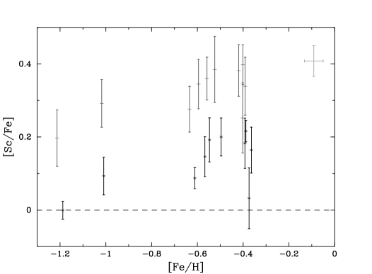
Therefore, we contend that there is an overabundance of Sc at [Fe/H] $\approx-0.5$ dex and await future observations at [Fe/H] $\approx-1$ to improve the statistical significance at that metallicity. It is interesting to note that our observations qualitatively match the [Sc/Fe] results from Prochaska & McWilliam (2000). In their reanalysis of Nissen et al. (2000), there is evidence for an enhancement of [Sc/Fe] near [Fe/H] $\approx-0.6$ yet no significant enhancement at [Fe/H] $\approx-1$. It is difficult to offer an explanation for the observed trend. Perhaps the Sc production in supernovae has a metallicity dependent yield. Or perhaps the enhancement at [Fe/H] $\approx-0.5$ is a statistical anomaly or is due to an overlooked source of systematic error.

Figure 14: Solar-corrected [V/Fe] abundance ratios vs. [Fe/H] metallicity for 9 of the 10 thick disk stars. The stars are all exhibit enhanced V and there is no obvious trend with metallicity. The dashed line at [V/Fe] = 0 indicates the solar meteoritic V/Fe ratio.

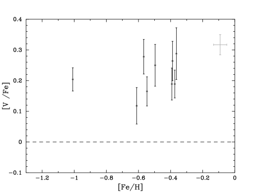
5.4.2 Vanadium

Even though there is an exhaustive list of useful V I lines (Whaling et al., 1985), there have been only a few studies of vanadium to date. Gratton & Sneden (1991) have observed V in a sample of $\approx 20$ stars with a large range in metallicity. Their analysis reveals no significant departure from the solar V/Fe ratio at any metallicity. As with many of the other iron-peak elements, V suffers from significant hyperfine splitting and we have been careful to account for it. To our surprise, our solar analysis of vanadium based on over 15 clean V I lines suggest a small but significant offset from the meteoritic value: ${\epsilon({\rm V})}_{\odot}=3.90\pm 0.014$. This is contrary to the results of Whaling et al. (1985) who derive ${\epsilon({\rm V})}_{\odot}=3.99\pm 0.01$, even though we adopt identical $\log gf$ values and our solar $W_{\lambda}$ measurements are larger. The discrepancy is eliminated, however, when we repeat the analysis with the Holweger & M$\ddot{\rm u}$uller (1974) solar atmosphere and the microturbulence value adopted by Whaling et al. (1985). In short, the V I lines are very sensitive to the temperature of the stellar atmosphere and even the small differences between the Kurucz and Holweger-M$\ddot{\rm u}$ller solar atmospheres lead to a 0.1 dex offset. In terms of the abundance analysis of the thick disk stars relative to the Sun, however, the relevant quantity is V/Fe which differs by $<0.05$ dex for the two models.

In Figure 14, we plot the solar-corrected [V/Fe] ratios versus [Fe/H] metallicity for the 9 stars with V I measurements. Every star exhibits an enhanced V/Fe ratio with no apparent trend with metallicity: $<[{\rm V/Fe}]>=+0.22\pm 0.02$. If anything, one might have expected a deficiency for vanadium as predicted by Timmes et al. (1995) in their chemical evolution model. In fact, this marks the first conclusive evidence for enhanced V/Fe ratios in any stellar population. We have carefully checked and rechecked our analysis for all possible systematic errors. For the stars with [Fe/H] $\approx-0.5$, the V/Fe ratio does depend on $T_{eff}$ ($\Delta$[V/Fe] $\approx+0.03$ for $\Delta T_{eff}=50$K), but it would require a very large temperature error to explain the entire enhancement. Therefore, we believe the V/Fe enhancement is a robust result and a very puzzling one at that. In $\S$ 6 we speculate on possible explanations.

Figure 15: Solar-corrected ($\times$) and standard (+) [Mn/Fe] abundance ratios vs. [Fe/H] metallicity for the 10 thick disk stars. The stars are all deficient in Mn and there is a mild trend toward lower [Mn/Fe] at lower metallicity. The dashed line at [Mn/Fe] = 0 indicates the solar meteoritic Mn/Fe ratio.

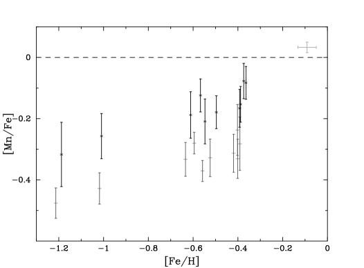
5.4.3 Manganese

Previous studies on manganese have indicated that it is underabundant relative to Fe in metal-poor stars (Wallerstein, 1962; Gratton, 1989). This trend has often been cited as evidence for the ’odd-even effect’ of $\alpha$-elements suggested by Helfer et al. (1959). Because Mn is an odd-element it suffers from hyperfine splitting and even in the case of moderately saturated absorption lines the hfs corrections can be large ($>0.3$ dex). It is crucial, therefore, to carefully account for the hyperfine splitting (Prochaska & McWilliam, 2000). In our analysis we adopted the hfs lines tabulated in Appendix B and relied on laboratory $gf$ values (Booth et al., 1984a; Martin et al., 1988). In addition to the difficulties associated with hyperfine splitting, Mn is special for the fact that its photometric solar abundance is significantly discordant from the meteoritic abundance (Booth et al., 1984b). As noted in $\S$ 4, our solar analysis also indicates that the solar photometric Mn value is significantly lower than the meteoritic, ${\epsilon({\rm Mn})}_{phot}-{\epsilon({\rm Mn})}_{meteor}\approx-0.2$ dex. We expect (as hypothesized by Booth et al. 1984b) that there is a zero-point error to the $\log gf$ values and, therefore, it is essential to consider a comparison relative to solar. Figure 15 plots the [Mn/Fe] values for our sample as a function of [Fe/H] for the standard (+) and solar-corrected ($\times$) analyses. In agreement with other studies of Mn in metal-poor stars (Gratton, 1989), we find sub-solar [Mn/Fe] values and evidence for a trend toward lower [Mn/Fe] values at lower metallicity.

Figure 16: Solar-corrected [Co/Fe] abundance ratios vs. [Fe/H] metallicity for the 10 thick disk stars. The stars are all exhibit enhanced Co and there is no obvious trend with metallicity. The dashed line at [Co/Fe] = 0 indicates the solar meteoritic Co/Fe ratio.

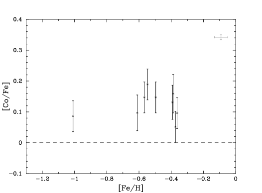
5.4.4 Cobalt

Cobalt is yet another odd-proton element in the iron-peak which suffers from hyperfine splitting. For our stars the hfs corrections are small, in particular because the typical equivalent widths of the Co I lines are small: $W_{\lambda}<30$ mÅ. With the exception of the most metal-poor star in our sample (G84-37), the [Co/Fe] measurements are based on $\approx 10$ absorption lines in good agreement ($\sigma<0.1$ dex). Although the solar photospheric ${\epsilon({\rm Co})}$ values are in good agreement with the solar meteoritic value ($\S$ 4), we plot the solar-corrected [Co/Fe] values in Figure 16 because the solar corrections significantly reduce the observed scatter. We find a clear enhancement of Co relative to Fe with no significant evidence for a trend with metallicity: $<$[Co/Fe]$>\;=+0.14\pm 0.02$ dex. The observed enhancement disagrees with the analysis of Gratton & Sneden (1991) who found that Co was actually underabundant relative to Fe by $\approx 0.1$ dex over the same metallicity range. As Tables 5 and 6 indicate, the CoI/Fe ratio is very insensitive to uncertainties in the atmospheric models, therefore uncertainties in the equivalent width measurements are the dominant source of error. Nonetheless, we find good agreement among the individual ${\epsilon({\rm Co})}$ measurements and have strong confidence in this result. This small enhancement hints at the significant overabundance of Co/Fe observed in the extremely metal-poor halo stars (McWilliam et al., 1995b).

Figure 17: Solar-corrected [Cu/Fe] abundance ratios vs. [Fe/H] metallicity for the 10 thick disk stars. With the exception of the most metal-poor star, all of the stars exhibit solar Cu/Fe ratios and there is no significant trend with metallicity. The dashed line at [Cu/Fe] = 0 indicates the solar meteoritic Cu/Fe ratio.

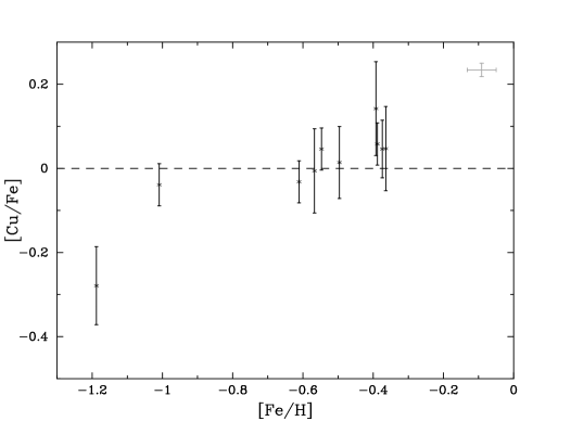
5.4.5 Copper

In very metal-poor stars, Sneden & Crocker (1988); Sneden et al. (1991) found copper to be deficient relative to iron, reaching [Cu/Fe] $\approx-1$ dex at [Fe/H] $\approx-3$. At metallicities comparable to our stars, however, their results show no significant departures from the solar ratio. Our observations include coverage of four Cu I absorption lines: $\lambda 5105,5218,5782,8092$. The first three have laboratory $gf$ measurements (Kock & Richter, 1968; Hannaford & Lowe, 1983) but there is considerable disagreement over the values ($\log gf$ for $\lambda 5782$ differs by $\approx 0.5$ dex). An analysis relative to solar is essential and given that we will rely on solar $gf$ values we also include Cu I $\lambda 8029$ in the analysis. Unfortunately, the solar equivalent width for $\lambda 5782$ is poorly constrained and we have excluded this line from the abundance analysis altogether. Copper suffers from significant hyperfine splitting and we have been careful to account for the effects in our analysis. Figure 17 presents the results from the solar-corrected analysis. While the uncertainties are large, the general picture is that the majority of stars show nearly solar Cu abundances with the marked exception of the most metal-poor star in our sample. There is an indication for a mild decrease in [Cu/Fe] with decreasing metallicity and the supersolar values at [Fe/H] $\approx-0.4$ suggest a small zero point error (0.05 dex) in our solar $gf$ values.

Figure 18: Solar-corrected [Zn/Fe] abundance ratios vs. [Fe/H] metallicity for the 10 thick disk stars. The majority of stars show enhanced Zn/Fe and there is no trend with metallicity. The dashed line at [Zn/Fe] = 0 indicates the solar meteoritic Zn/Fe ratio.

5.4.6 Zinc

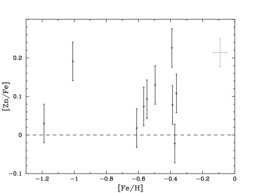
In their comprehensive study of Zn, Sneden & Crocker (1988); Sneden et al. (1991) found a nearly solar Zn/Fe ratio over a large range of metallicity: $<[{\rm Zn/Fe}]>_{Sneden}=0.04\pm 0.02$. We have analyzed the same two Zn I lines as Sneden et al. (1991) and adopted the theoretical $gf$ values (Bi$\rm\acute{e}$mont & Godefroid, 1980). Even though our solar analysis is in excellent agreement with the solar meteoritic value, we noticed that the $\lambda 4722$ line yields systematically higher ${\epsilon({\rm Zn})}$ values while the $\lambda 4810$ line gives systematically lower ${\epsilon({\rm Zn})}$. We recommend that the oscillator strengths be adjusted by 0.04 dex as follows: $\log gf_{\lambda 4722}=-0.35$, $\log gf_{\lambda 4810}=-0.21$. The agreement of the two lines for the thick disk stars after the correction was generally $<0.02$ dex. Therefore the error bars plotted in Figure 18, which represent the scatter in ${\epsilon({\rm Zn})}$ from the two Zn I lines, underestimate the true uncertainty in [Zn/Fe] which is dominated by the error in $T_{eff}$ ($\pm 0.03$ for $\Delta T=50$K). Figure 18 gives the [Zn/Fe] values for the 10 thick disk stars vs. [Fe/H]. Three of the stars exhibit Zn/Fe values consistent with the solar ratio, yet the majority are enhanced relative to solar with two stars showing enhancements of $\approx$ +0.2 dex. The mean enhancement is $<$[Zn/Fe]$>\,=0.093\pm 0.025$, which is larger than the value reported by Sneden et al. (1991). While the enhancement may be unique to thick disk stars, there are also indications of an overabundance of Zn in very metal-poor stars (Johnson, 1999). Given the tremendous impact of this ratio on studies in the damped Ly$\alpha$ systems, it will be very important to repeat a survey similar to Sneden et al. (1991) with more accurate Fe abundances and modern model atmospheres. It is worth noting that an overestimate in $T_{eff}$ of 100K (as might be the case for the majority of our stars), would imply an increase in the [Zn/Fe] abundances by 0.06$-$0.08 dex implying a mean [Zn/Fe] enhancement of $+0.15-0.17$ dex.

Figure 19: Solar-corrected ($\times$) and standard (+) [Ba/Fe] abundance ratios vs. [Fe/H] metallicity for the 10 thick disk stars. The observations show a mild enhancement which we do not believe is statistically significant (see the text). The dashed line at [Ba/Fe] = 0 indicates the solar meteoritic Ba/Fe ratio.

5.5 Heavy Elements – Ba, Y, Eu

Unfortunately, due to the lack of available absorption lines we have only been able to obtain abundance measurements for three heavy elements: Ba, Y, and Eu. These abundances are derived from very few lines and are poorly constrained. Nonetheless, they provide tentative insight into the relative importance of the r and s-processes in these thick disk stars.

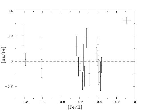
While barium can be synthesized through both the s and r-processes, it is believed that the solar system composition is $\approx 90\%$ s-process (Kappeler et al., 1990) and one expects barium to be synthesized primarily via the s-process in metal-poor stars. Our spectra include coverage of four Ba II lines: $\lambda 4554,5853,6141,6496$. The first absorption line is heavily saturated for all of the thick disk stars so the analysis focuses only on the latter three for which we adopt $gf$ values from McWilliam (1998). Because barium suffers from significant hyperfine splitting, we carefully calculated hfs corrections with the hfs lines presented in Table 11 taken from McWilliam (1998). For the hfs corrections we have adopted an r-process isotopic composition and we note that the s-process composition increase ${\epsilon({\rm Ba})}$ by less than 0.03 dex. For the solar analysis, $\lambda 6141$ was too saturated to provide an accurate correction. Furthermore, we estimate the correction for $\lambda 6496$ to be very large, perhaps the result of an unidentified blend. In terms of the thick disk abundance analysis, the solar-correction analysis leads to a decrease in the typical [Ba/Fe] value by $0.17$ dex. Figure 19 plots the standard and solar-corrected values which yield mean values $<[{\rm Ba/Fe}]>\,=0.093\pm 0.024$ and $<[{\rm Ba/Fe}]>\,=-0.077\pm 0.017$ respectively. The offset between the two is large and worrisome. Our best interpretation of the overall results is that the stars exhibit nearly solar Ba/Fe although a further investigation is warranted. For the discussion in the following section, we will use the uncorrected barium abundances as we fear the solar analysis introduces too large an uncertainty.

Figure 20: Standard (uncorrected) [Y/Fe] abundance ratios vs. [Fe/H] metallicity for the 10 thick disk stars. All of the observations are consistent with the solar ratio. The dashed line at [Y/Fe] = 0 indicates the solar meteoritic Y/Fe ratio.

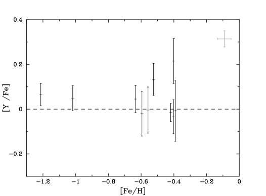
Previous analyses on yttrium (Zhao & Magain, 1991; Gratton & Sneden, 1994) have demonstrated a mild metallicity dependence of [Y/Fe] with [Fe/H] where metal-poor stars show mildly deficient Y. These studies focused on Y II lines which are plentiful and for which a reasonably large database of $gf$ values exist (Hannaford et al., 1982). While we observed $\approx 10$ Y II lines for each star, almost every line suffers from significant line blending. Therefore the final Y/Fe abundance measurements are based on only $1-3$ clean Y II lines. Because the solar-corrected analysis further reduces the number of lines considered and does not give significantly different results from the standard analysis, we present the uncorrected [Y/Fe] values in Figure 20. All of the Y/Fe values are consistent with the solar ratio and we observe no trend with metallicity. Note that the high [Y/Fe] measurement from G97-15 was derived from a single Y II line which is partially blended.

Figure 21: Standard (uncorrected) [Eu/Fe] abundance ratios vs. [Fe/H] metallicity for the 4 stars with wavelength coverage of the Eu II $\lambda 6645$. All of the observations are significantly enhanced above the solar ratio. The dashed line at [Eu/Fe] = 0 indicates the solar meteoritic Eu/Fe ratio.

Europium is predominantly synthesized through the r-process. Because the r-process takes place almost exclusively in Type II SN, Eu should trace other elements formed primarily through Type II SN (i.e. the $\alpha$-elements). Unfortunately, the observational challenge for a europium abundance analysis in the thick disk stars is severe. While we have coverage of Eu II $\lambda 6437$, it was too weak to reliably measure. Furthermore, the Eu II $\lambda 6645$ line lies at the red edge of our setup and could be measured only in those stars with geocentric velocity $v<60{\rm\;km\;s^{-1}}$. Finally, the Eu II $\lambda 6645$ line is very weak and given that it is found near the end of a spectral order, its equivalent width is particularly uncertain: $\sigma(W_{\lambda})>3$mÅ. We find [Eu/H] $\approx+0.1$ based on a solar analysis of $\lambda 6645$ but consider this value to be unreliable. Therefore we present the standard results in Figure 21 and warn that they may be systematically high by $\approx 0.1$ dex. We observe Eu to be significantly enhanced in these stars, $<[{\rm Eu/Fe}]>\,=0.47\pm 0.05$. Unfortunately, there are too few measurements from our sample to meaningfully comment on any trend in [Eu/Fe].

5.6 Summary

Table 10 provides a summary of the abundance measurements for the thick disk sample. Column 1 lists element X, column 2 details the number of stars ($N$) with measurements of X, column 3 gives the mean [X/Fe] ratio $\bar{x}$, column 4 is the error in the mean $\sigma(\bar{x})$, column 5 marks whether the abundances were corrected by the solar analysis $(\odot$), column 6 indicates if we believe a trend of [X/Fe] with [Fe/H] metallicity is likely, and column 7 provides additional comments. Forgoing a formal error analysis to future papers, the error in the mean merely represents the reduced standard deviation: $\sigma(\bar{x})=\sigma/\sqrt{N-1}$. This value is more representative than the formal statistical error given the many systematic uncertainties involved in measuring the abundance of a given star. We warn, however, that systematic errors which affect all of the measurements – $gf$ offsets, errors in the Kurucz atmospheres, etc. – may exceed the $\sigma(\bar{x})$ values.

Table 10: ABUNDANCE SUMMARY

X	$N$	$\bar{x}$	$\sigma(\bar{x})$	Trend	App
O	10	$0.488$	0.056	y
Na	10	$0.101$	0.017	n	$\odot$
Mg	10	$0.371$	0.017	n
Al	9	$0.334$	0.028	n	$\odot$
Si	10	$0.172$	0.021	?	$\odot$
S	9	$0.111$	0.075	?	$\odot$
Ca	10	$0.197$	0.020	y	$\odot$
Sc	10	$0.131$	0.025	?	$\odot$
Ti	10	$0.290$	0.021	n	$\odot$
V	9	$0.216$	0.020	n	$\odot$
Cr	10	$0.000$	0.011	n	$\odot$
Mn	10	$-0.175$	0.025	y	$\odot$
Co	9	$0.123$	0.015	n	$\odot$
Ni	10	$0.021$	0.007	n	$\odot$
Cu	10	$0.000$	0.037	y	$\odot$
Zn	10	$0.093$	0.025	n	$\odot$
Y	10	$0.043$	0.026	n
Ba	10	$0.094$	0.024	n
Eu	4	$0.475$	0.046	n

Figure 22: Abundance patterns for the thick disk stars (large black stars) for 18 of the elements analyzed in this paper. For comparison, we plot the abundance patterns for halo stars (green points), thin disk stars (red points), other thick disk measurements (small black stars), and a small sample of bulge stars (light blue points). The different symbols refer to the various literature sources indicated in the text. There are three principal points to take from the figure: (1) for many of the elements, the thick disk abundances are distinct from the thin disk; (2) the thick disk abundances tend toward the halo star values at [Fe/H] $\approx-1$; (3) the thick disk abundances are in good agreement with the bulge values for essentially every element.

Figure 23: Abundance patterns for the thick disk stars (large black stars) for 18 of the elements analyzed in this paper. For comparison, we plot the abundance patterns for halo stars (green points), thin disk stars (red points), other thick disk measurements (small black stars), and a small sample of bulge stars (light blue points). The different symbols refer to the various literature sources indicated in the text. There are three principal points to take from the figure: (1) for many of the elements, the thick disk abundances are distinct from the thin disk; (2) the thick disk abundances tend toward the halo star values at [Fe/H] $\approx-1$; (3) the thick disk abundances are in good agreement with the bulge values for essentially every element.

Figure 24: Abundance patterns for the thick disk stars (large black stars) for 18 of the elements analyzed in this paper. For comparison, we plot the abundance patterns for halo stars (green points), thin disk stars (red points), other thick disk measurements (small black stars), and a small sample of bulge stars (light blue points). The different symbols refer to the various literature sources indicated in the text. There are three principal points to take from the figure: (1) for many of the elements, the thick disk abundances are distinct from the thin disk; (2) the thick disk abundances tend toward the halo star values at [Fe/H] $\approx-1$; (3) the thick disk abundances are in good agreement with the bulge values for essentially every element.

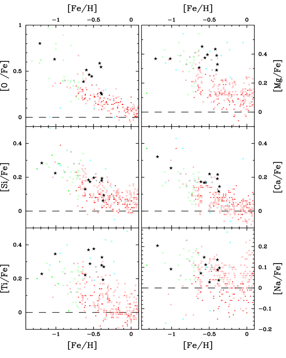
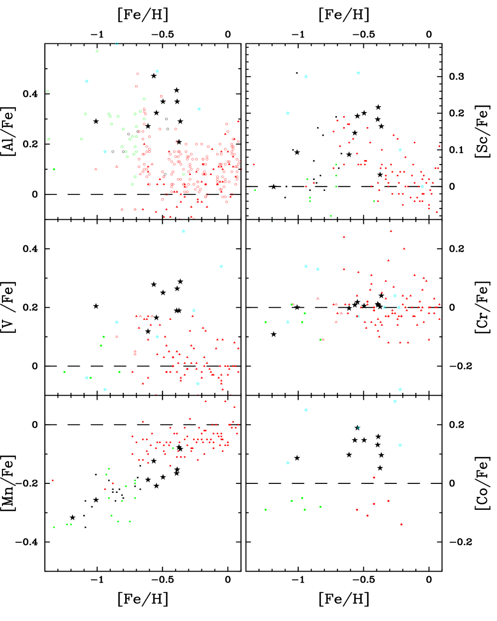
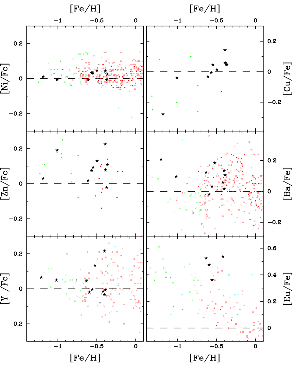
6 DISCUSSION

6.1 Comparisons with Other Stellar Populations

In the previous section, we presented an element-by-element account of the abundances for the thick disk stars offering comparisons between our results and previous work. In this section we will contrast the elemental abundances against other stellar populations, namely the metal-poor halo stars, the thin disk stars, and a small sample of bulge stars. In the following subsections, we comment on the implications for the formation history of the thick disk and Galaxy as well as the nucleosynthesis of these elements in the early universe.

Figures 22-24 present abundances for 18 elements with our sample of thick disk stars plotted as large black stars. We do not include S in this subsection because of the very large uncertainties associated with these measurements in all stellar populations. In each sub-panel, we overplot abundance measurements taken from a number of literature sources which describe the metal-poor halo (green), the thin disk (red), the thick disk (black), and the bulge (light blue). Abundance trends are sensitive to the stellar atmosphere, spectrum synthesis algorithm, hyperfine splitting corrections, etc. adopted by each group and therefore systematic uncertainties exist in comparing various data sets. It is important at the least to keep this uncertainty in mind and if possible to correct for identifiable systematic offsets. The plot symbols distinguish the various data sets: (i) the Edvardsson et al. (1993) data are plotted as open circles. We have noted ($\S$ 3.4) a systematic offset between their temperature scale and ours of $\Delta T_{eff}\sim 100$ K. We correct for this offset by applying the values in Table 9 of Edvardsson et al. (1993) which gives the sensitivity of various element ratios on $T_{eff}$. We have identified thick disk stars in the Edvardsson et al. (1993) sample according to the same kinematic criteria imposed for our sample ($Z_{max}>600$ pc; $-100<\tilde{V}<-20$ km s^-1 ; $-1.1<{\rm[M/H]}<-0.4$). We also identified a few halo stars which have $\tilde{V}<-100{\rm\;km\;s^{-1}}$ and large eccentricity. The remaining stars are plotted as thin disk stars if [Fe/H] $>-0.7$ and as halo stars otherwise. We warn, however, that many of these stars at [Fe/H]$~{}\approx-0.7$ could be thick disk members. (ii) The triangles represent the chemical abundances from Chen et al. (2000). We believe Chen et al. (2000) adopted a similar temperature scale to ours so we make no correction to this data set. Chen et al. (2000) identified a small subsample of thick disk stars according to kinematic and metallicity criteria; these are plotted as open red triangles in the figure. As noted in the introduction, these stars have implied ages younger than that typically assumed for the thick disk and therefore we contend that they are actually thin disk stars; (iii) The solid circles depict the values taken from Gratton & Sneden (1988), Gratton & Sneden (1991), Sneden et al. (1991), and Gratton & Sneden (1994). Because these authors did not characterize these field stars according to specific stellar populations, we have plotted them under the assumption that those stars with [Fe/H] $<-0.7$ are halo stars and the remaining are thin disk stars. For the few stars near [Fe/H] $=-0.7$ it is possible that there is some contamination from thick disk stars; (iv) The Sc and Mn values (solid squares) are taken from Prochaska & McWilliam (2000) who reanalyzed the abundances reported by Nissen et al. (2000). As Prochaska & McWilliam (2000) emphasize, their values may not represent the true Mn and Sc abundances, but they should be more accurate than the Nissen et al. (2000) values which are based on an incorrect hfs treatment. For these measurements, we have adopted the stellar population identifications given by Nissen et al. (2000); (v) For the O abundances, we have restricted our comparisons to those measurements based on the O I lines at 7770 Å as there are concerns over systematic differences between the various approaches to measuring oxygen (Tomkin et al., 1992; Abia & Rebolo, 1989); (vi) The bulge abundances are taken from McWilliam & Rich (1994); and (vii) The open squares represent values taken from the remaining literature sources (Brown & Wallerstein, 1992; McWilliam et al., 1992; Shetrone, 1996). For all of the data sets we have normalized the measurements to the updated Grevesse et al. (1996) solar meteoritic abundance scale as necessary.

It is difficult to digest all of the abundance trends presented in Figures 22-24, yet several comparisons stand out. In terms of the $\alpha$-elements, the thick disk stars exhibit significantly larger overabundances than the thin disk stars. The O and Mg results agree with the overabundances claimed by previous thick disk studies (Gratton et al., 2000; Fuhrmann, 1998) while the Ca and Ti ratios lend even further support that the thick disk is chemically distinct from the thin disk. The Si/Fe ratios are the least enhanced over the thin disk, yet other than the two lowest Si/Fe values even these values are higher than the average thin disk star at [Fe/H] $\approx-0.5$. Therefore, the $\alpha$-elements offer convincing evidence that the thick disk population is chemically discrete from the thin disk. This point contradicts the interpretation of Chen et al. (2000) who comment that the thick disk abundances extend smoothly from the thin disk. As noted above, however, the Chen et al. (2000) sample of thick disk stars are younger than the fiducial age of the thick disk casting their conclusions into serious doubt. This point not withstanding, carefully examining Figures 22-24 one notes that the thick disk stars from Chen et al. (2000) all have metallicity [Fe/H] $<-0.6$ where a comparison with the thin disk is difficult owing to the paucity of measurements of thin disk stars with [Fe/H] $<-0.6$. In contrast with the thin disk, the halo star values are in much better agreement with the thick disk stars. The Mg and Ti abundances show similar enhancements for the two populations while the remaining $\alpha$-elements approach the halo star values in the most metal-poor thick disk stars. Finally, we find an impressive match between the bulge and thick disk $\alpha$-element abundances. The Ca, Mg, and Ti trends are all in agreement, while the thick disk Si abundances show somewhat smaller enhancements. To summarize our results on the $\alpha$-elements, of the four stellar populations the thick disk and bulge star abundance patterns most resemble one another, the most metal-poor thick disk stars closely match the halo values, and all of these populations show $\alpha$-enhancements which are significantly larger than the values observed for thin disk stars.

As with the $\alpha$-elements, the light elements – sodium and aluminum – are enhanced in the thick disk stars. The Na/Fe results are in good accord with the Edvardsson et al. (1993) analysis yet contradict the results from Chen et al. (2000). Chen et al. (2000) noted this discrepancy between their results and Edvardsson et al. (1993), but did not determine the cause. With respect to the halo and bulge, the thick disk values are somewhat larger than the typical halo values (either solar or sub-solar) and the Na/Fe values from the metal-poor bulge stars (based on only 1 or 2 Na I lines). Given the large uncertainties associated with measuring Na in each of these stellar populations, we do not feel confident in drawing any conclusions aside from the observation that none of the populations show significant Na/Fe departures from the solar ratio. The Al measurements, on the other hand, offer more compelling comparison. The thick disk Al abundances are enhanced over the thin disk observations by both Chen et al. (2000) and Edvardsson et al. (1993) and are in reasonable agreement with the halo star observations. Finally the majority of Al measurements from the bulge stars match the thick disk, although there are several bulge measurements with [Al/Fe] $>+0.6$ dex.

With respect to the iron-peak measurements of the thick disk, the Ni, Cu, and Cr abundances generally track Fe, yet the remaining elements all show significant departures from the solar abundance. In several ways, the thick disk stars significantly distinguish themselves from the halo and thin disk stellar populations. First, unlike the thin disk the V, Co, and Zn abundances are all enhanced in the thick disk. Second, all but two of the thick disk stars exhibit significantly lower Mn/Fe ratios than the thin disk. Whereas the thin disk and halo appear to exhibit plateaus in [Mn/Fe] at $-0.05$ and $-0.3$ dex respectively, the thick disk values show a trend with metallicity which connects the other two populations. In the case of Zn, V, and Co, the thick disk ratios are even enhanced over the halo abundances for halo stars with [Fe/H] $\geq-1.8$ (the extremely metal-poor halo stars also have overabundances of Co and Zn; McWilliam et al. 1995, Johnson 1999). As discussed in $\S$ 5.4.1, the thick disk Sc/Fe results are very peculiar. The stars with [Fe/H] $\approx-0.5$ dex show a marked Sc/Fe overabundance while the two metal-poor stars have nearly solar Sc/Fe ratios. These results are in surprisingly good agreement with the Sc/Fe results from Prochaska & McWilliam (2000). The Sc abundances are very unusual and require further investigation before one can meaningfully comment on their implications. Given the significant number of distinctions between the thick disk and the halo/thin disk stellar populations, the agreement between the iron-peak abundance patterns of the thick disk and bulge is stunning. In particular, the metal-poor bulge stars show enhancements in V and Co at levels consistent with the thick disk results and there is even an indication of enhanced Sc. It must be noted, however, that the iron-peak bulge values are primarily based on 1-2 lines and that McWilliam & Rich (1994) did not take particular care to account for line blending. The latter point, in particular, gives pause because with the exception of Mn the iron-peak abundances we are considering are enhanced. We anxiously await confirmation of these trends by McWilliam & Rich (2000) who have recently obtained a sample of bulge stars observed with HIRES on Keck I at significantly higher resolution than their previous study.

Finally, we can compare the various stellar populations with respect to the heavy element abundance trends. This is somewhat ambitious, however, given the large uncertainties of our Ba, Y, and Eu measurements. Nevertheless, the Ba and Y trends are in reasonable agreement for all of the stellar populations in this metallicity range; in general, they are all consistent with the solar composition. Europium, however, presents a different story. In agreement with the the $\alpha$-element observations and the notion that Eu is formed predominantly in Type II SN, the thick disk Eu/Fe ratios are well in excess of the thin disk measurements and comparable to the halo and bulge values.

6.2 Implications for the Formation of the Thick Disk

In the previous subsection, we drew comparisons between the abundance patterns of the thick disk stars with the halo, thin disk, and bulge stellar components. For the majority of elements – the $\alpha$-elements, Co, V, Zn, Al, Mn, Eu – the thick disk stars show abundance patterns which clearly distinguish them from the thin disk. These results provide compelling confirmation that the chemical history of the two stellar components is distinct as first suggested by the Mg and O analysis of Gratton et al. (2000) and Fuhrmann (1998). In turn, our analysis implies the thick disk is a physically distinct stellar component from the thin disk with its own specific formation history.

Gratton et al. (2000) and Fuhrmann (1998) have further argued that the discrete separation of the O/Fe and Mg/Fe ratios between the two stellar populations implies a significant time delay between the formation of the thick disk and the onset of star formation in the thin disk. This assertion appears well supported by our results. The larger $\alpha$/Fe enhancement demonstrated in the thick disk indicates the thin disk stars formed from gas more significantly polluted by Type Ia SN requiring a significant delay between the formation epochs. As described below, however, this assertion is now complicated by the tentative evidence for Type Ia contributions in the thick disk abundance patterns. Nevertheless, the fact that the thick disk abundance patterns do not smoothly transition to the thin disk does require a significant delay in the star formation rate following the formation of the thick disk stars. The overabundance of the $\alpha$-elements in the thick disk as well as the underabundance of Mn/Fe indicate that the thick disk formed prior to the thin disk on the grounds that there was less pollution from the long-lived Type Ia SN. In addition, the observed halo-like Ba/Eu ratio (Figure 25) indicates r-process dominated enrichment which supports a great age for these stars.

In the abundance studies by Gratton et al. (2000) and Fuhrmann (1998) there is no indication for a trend of [O/Fe] or [Mg/Fe] with metallicity. Gratton et al. (2000) therefore asserted that the formation of the thick disk occurred on time-scales shorter than the Type Ia SN, i.e. $t_{form}<1$ Gyr. If confirmed, the tentative trends of Ca, Si, and O with metallicity in our sample of thick disk stars contradict this assertion. Traditionally, the decrease of an $\alpha$-element enhancement with increasing [Fe/H] metallicity is attributed to the onset of Type Ia SN. This explanation is well motivated by our theoretical understanding of Type Ia and Type II SN. If it explains the Si, Ca, and O trends for the thick disk, it will be difficult to reconcile our observations with the notion of a brief thick disk formation time. Instead the observed $\alpha$-element trends may indicate that the formation time of the thick disk exceeds the Type Ia SN timescale, i.e. $t_{form}\gtrsim 1$ Gyr. To reconcile the nearly constant Mg/Fe trend under this scenario, however, one may require fine tuning in the form of enhanced formation of very massive Type II SN, an enhanced production factor for Mg in metal-poor Type Ia SN, or increased Mg production in more metal-rich Type II SN. Another possibility altogether is that the $\alpha$-element trends are the sole result of Type II SN with an evolving IMF; specifically, the importance of the moderate mass Type II SN decreases as [Fe/H] increases. In this case, $t_{form}\ll 1$ Gyr, but it is difficult to understand the O/Fe trend with [Fe/H]. In the following, we will adopt the hypothesis that the O,Si, and Ca trends imply $t_{form}\gtrsim 1$ Gyr but warn that further investigation into the nucleosynthetic history of the thick disk is crucial.

To date, several scenarios have been put forward to explain the formation of the thick disk. In particular, these include dissipative collapse models (Larson, 1976; Jones & Wyse, 1983), dynamical heating (Noguchi, 1998), and merger scenarios (Quinn et al., 1993; Huang & Carlberg, 1997; Sellwood et al., 1998). Our observations place important constraints on these models. Consider first the formation of the thick disk during the dissipative collapse of a gaseous halo. In order to maintain the chemical (and kinematic) distinction between the thick and thin disks, the thick disk must form prior to the thin disk, in situ from a gaseous disk with a velocity dispersion consistent with the thick disk stars $(\sigma_{W}\approx 40{\rm\;km\;s^{-1}}$). As suggested by Jones & Wyse (1983), this may be the natural evolution of a gaseous halo which has undergone some initial dissipation. The dissipational time-scale, however, is significantly shorter than 1 Gyr, i.e. $t_{form}\ll 1$ Gyr in the dissipational collapse scenario. One could invoke additional energy sources such as primordial magnetic fields (Jedamzik et al., 1999) or an enhanced supernovae rate and demand that they maintain the 40 km s^-1 velocity dispersion of the gas disk for 1 Gyr while allowing the dissipational collapse and formation of molecular clouds and stars, but this is unlikely. On the grounds that the formation time of the thick disk might well exceed 1 Gyr, we contend it is unlikely that the thick disk formed in situ as envisioned in an ELS-like scenario. Therefore, the thick disk must have been preceded by a stellar thin disk which was heated – either gradually over the course of $\approx 1$ Gyr or suddenly – to the current thick disk. The clumpy star-forming region model envisioned by Noguchi (1998) provides a gradual heating mechanism ($t_{form}\approx 1$ Gyr) for the formation of the thick disk. In this model, $10^{9}M_{\odot}$ clumps form during the dissipational collapse of the Galaxy which initiate star formation, spiral to the galaxy center via dynamical friction, scatter the stars in the initial thin disk to form a thick disk, and eventually merge to form the bulge. The model does not describe the formation of the current thin disk; presumably it will form after the clumps have merged through the accretion of a new reservoir of gas, but this may require some fine tuning to insure that the resulting thin disk is chemically distinct from the thick disk. This complication aside, the model accounts for the majority of our observations. Finally, consider merging scenarios where the initial thin disk is heated via the accretion of one or more satellites. Unfortunately, it is difficult to assess this model as the various numerical studies conflict on the effects of a merger event (e.g. heating efficiency; Quinn et al. 1993; Huang & Carlberg 1997; Sellwood et al. 1998). Nonetheless, this scenario should naturally allow for the formation of the initial thin disk over the course of 1 Gyr and the merger event(s) would erase all trace of the initial thin disk providing the discrepancy between the resulting thick disk and the future thin disk. Similar to the clumpy region model, however, the formation of the thin disk after the merger event has not been considered in these numerical simulations. Furthermore, they disagree on the robustness of the thick disk to future accretion events. Hopefully, future numerical simulations will resolve the current conflicts and pursue the formation of both the thick and thin disks.

What does a comparison of the thick disk with the halo chemical abundances reveal? It is informative that with the exception of Co and V (and maybe Zn) the thick disk abundances for all of the elements match or approach the abundances of halo stars with [Fe/H] $\approx-1.3$. This implies that the metal-poor thick disk stars formed from similar material as that for the most metal-rich halo stars. This naturally follows from the notion that the halo stars formed first, i.e., before the majority of gas had dissipated to form a disk (thin or thick). Subsequently, those stars which formed first in the disk exhibit abundances similar to the metal-rich halo stars while the later disk stars show higher metallicity and evolved abundance patterns. This explanation does not account for the discordant Co and V trends. Perhaps these abundances are the result of a specific type of nucleosynthesis event (e.g. supernova) whose time-scale exceeds the formation of the halo. Alternatively, the overproduction of these elements may require specific physical conditions (i.e. surface density, binary fraction, metallicity) which did not exist in the halo. Therefore, by identifying the mechanisms responsible for the Co and V enhancements, one might gain further insight into the time-sequence of the formation of the Galactic halo and thick disk.

The similarities of the thick disk and bulge chemical abundance patterns are striking. With the exception of the O/Fe (which can be disregarded) and possibly the Si/Fe ratios, there is no significant difference in the abundance patterns of any element. The obvious interpretation of this agreement is that the two stellar components formed at essentially the same time and from the same gas reservoir. It is also interesting to note that the presence of thick disk in external galaxies has been linked to systems with significant bulges (Burstein, 1979). The most straightforward explanation is that a single merger event sparked the formation of both stellar components, although this is not the only possibility. The two components may have formed together through a lengthy dynamical process as described by Noguchi (1998). It is also worth noting that the dissipational collapse model of Jones & Wyse (1983) also predicts a close association between the metal-poor bulge stars and the thick disk. Nevertheless, the claim that the two components shared a similar gas reservoir and formation epoch is largely independent of the exact physical processes involved in their formation. We eagerly look forward to future analyses of the bulge (McWilliam & Rich, 2000), in particular the metal-poor tail. If these observations confirm the current picture (in particular the Co and V enhancements), the two stellar components will be irrefutably wed and all viable Galactic formation scenarios will need to account for them simultaneously.

6.3 Implications for Nucleosynthesis

Irrespective of comparisons with other stellar populations, the chemical abundances of the thick disk stars provide unique constraints on the processes of nucleosynthesis in the early universe. Consider first the $\alpha$-elements which exhibit an overabundance relative to Fe for all of the thick disk stars; the enhancements indicate that the gas from which these stars formed was primarily enriched by Type II SN. Furthermore, by comparing the various abundance trends of the $\alpha$-elements one gains insight into the yields from different mass and/or metallicity Type II SN. As noted in the previous subsection, the most striking comparison is that the Mg and Ti abundances show no dependence on [Fe/H] metallicity whereas the Ca, Si, and O ratios appear to decrease steadily with increasing [Fe/H] for the thick disk stars. While this statement is largely dependent on the observations of the two metal-poor stars in our sample and therefore suffers from small number statistics, we speculate on the implications. Differences between the trends of Mg and Si or Ca may be expected on theoretical grounds because these elements are believed to be synthesized in different mass Type II SN (Woosley & Weaver, 1995). In particular, the SN models suggest that Mg is produced primarily in the highest mass Type II SN whereas the production of Si and Ca is dominated by moderate mass SN. The observed trends, however, are difficult to explain under the assumption of a constant IMF. If anything, one might expect significant evolution in Mg as it arises in the more massive Type II SN. Therefore, either nucleosynthesis occured in Type II SN with an evolving IMF or Type Ia SN are playing a significant role in the observed abundance trends. If the latter explanation is adopted (as assumed in the previous subsection), then it becomes a challenge to explain the constancy of the Mg/Fe ratio. Perhaps at [Fe/H] $\approx-0.5$ there is an increase in the number of very massive Type II SN or maybe the the first generation of Type Ia SN overproduces Mg. It is also difficult to reconcile the difference in the Mg and O abundance trends as both elements are expected to be produced primarily in massive Type II SN and therefore should track one another reasonably well. It is possible the O trend is the result of a systematic error (i.e. non-LTE effects) in measuring O from the O I triplet at $\lambda\approx 7775$Å. If this is not the case, the observations pose a meaningful challenge to the current models of Type II SN. Finally, while the similarity between the Mg and Ti trends may be a coincidence, it does suggest the possibility that the two elements are produced in similar nucleosynthetic sites. At the very least, while searching for the processes which yield enhanced Ti one may wish to first focus on those mechanisms which produce Mg.

The behavior of the light elements in the thick disk stars differs considerably. The Na/Fe ratios follow the $\alpha$-element enhancements – albeit with a more mild overabundance – in a fashion possibly consistent with some Type II SN contribution. The enhancement is small, however, and could be the result of a systematic error in the Na analysis. In contrast, aluminum is significantly enhanced over the solar ratio which clearly points to a significant production of Al in massive stars. Like Mg and Ti, Al exhibits no obvious trend with [Fe/H] metallicity in our sample. Again, we can speculate that Al is formed in similar sites as Mg and Ti.

With respect to nucleosynthesis, the abundance trends of several of the iron-peak elements may offer the most startling results. In particular, the thick disk stars show enhanced Co and V where if anything one predicts a deficiency for these ’odd’ nuclei. Furthermore, the Zn enhancement – while mild – appears to contradict the previous empirical belief that Zn/Fe is solar at all metallicities. The Co enhancement brings to mind the overabundance observed for extremely metal-poor stars (McWilliam et al., 1995b). Cobalt is believed to be synthesized during the $\alpha$-rich freeze out fueled by a neutrino-driven wind (Woosley & Hoffman, 1992). An enhancement of Co might then be expected to be correlated with other elements slightly more massive than Fe. Similar to the extremely metal-poor stars, however, we do not observed enhanced Ni or Cu, yet we note that the Zn enhancement (also seen in the extremely metal-poor stars; Johnson 1999) could be related to the Co pattern. It will be important to focus on the Co/Zn ratio in future studies. The vanadium overabundance is not predicted by any current theoretical model of nucleosynthesis. According to Woosley & Weaver (1995), the dominant vanadium isotope ${}^{51}{\rm V}$ is primarily produced during the $\alpha$-rich freeze out, yet the leading theories predict only a fraction of the observed solar vanadium abundance (Woosley, 1986). In fact, to the best of our knowledge this marks the first significant evidence for enhanced V in any stellar population. The V overabundance poses an excellent challenge for nucleosynthesis research on an element which until now has been largely ignored. Finally, note that the unusual Sc/Fe trends agree surprisingly well with the reanalysis of Nissen et al. (2000) by Prochaska & McWilliam (2000). The trend is very peculiar with the [Fe/H] $\approx-1$ stars exhibiting essentially no Sc/Fe enhancement, most stars at [Fe/H] $\approx-0.5$ enhanced above solar, and the nearly solar metallicity stars show solar Sc/Fe. As with Co and V, scandium is believed to be produced primarily through the $\alpha$-rich freeze out process. Given the very unusual behavior of Sc/Fe, a combination of metallicity dependent yields and various supernovae appears likely. Perhaps the overabundance at [Fe/H] $\approx-0.5$ is due to the onset of Type Ia SN whose relative Sc/Fe production decreases with increasing metallicity. Altogether, the Co, V, Sc, and Zn enhancements point toward a further investigation of the $\alpha$-rich freeze out nucleosynthesis. In turn, one may learn about the IMF of the thick disk stars. Finally, we note that the Mn/Fe values for the thick disk are generally lower than the thin disk values. We consider this evidence for the overproduction of Mn in Type Ia SN (Gratton, 1989). This assertion is further supported by the fact that the stars with the highest Mn/Fe ratios show the lowest Si/Fe, Ca/Fe, and O/Fe values and argue against a metallicity dependent yield for Mn.

Figure 25: [Ba/Eu] ratios vs. [Fe/H] metallicity for the 4 stars with measured Eu abundance. Overplotted in the figure are the fiducial values for the s and r-process Ba/Eu ratios. The results suggest a mix of the two processes with the r-process being dominant.

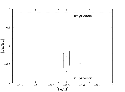
We conclude our discussion of nucleosynthetic implications with a few comments on the heavy element results. Figure 25 presents the [Ba/Eu] ratio against [Fe/H] for the four stars with wavelength coverage of the Eu II $\lambda 6645$ line. Overplotted on the figure are two lines indicating the fiducial values for the solar s and r-process values of the Ba/Eu ratio. The thick disk ratios lie in between the two fiducial values suggesting that both processes are important in the nucleosynthesis of the heavy elements, although the r-process appears dominant. As noted in the previous section, this is consistent with the very large age believed for the thick disk stars. Lastly, the Ba/Y ratio is approximately solar in line with the halo composition (Gratton & Sneden, 1994).

6.4 Comparisons with the Damped Ly$\alpha$ Systems

This final section describes the implications of our results on interpretations of the abundance patterns of the damped Ly$\alpha$ systems. The damped Ly$\alpha$ systems are absorption line systems identified along the sightlines to distant quasars and have neutral hydrogen column densities ${N({\rm HI})}\geq 2{\rm\;\times\;10^{20}}\,{\rm cm^{-2}}$. Owing to their very large ${N({\rm HI})}$ values, these systems dominate the neutral hydrogen content of the universe at all epochs (Wolfe et al., 1995; Rao & Turnshek, 2000). Furthermore, the very large column densities imply overdensities suggestive ($\delta\rho/\rho\gg 100$) of protogalaxies. Finally, the comoving baryonic mass density in gas inferred from the damped systems at $z=2-3$ coincides with the current comoving baryonic mass density in stars today (Wolfe et al., 1995; Storrie-Lombardi and Wolfe, 2000). For these reasons the damped Ly$\alpha$ systems are widely believed to be the progenitors of modern galaxies. The majority of studies on the chemical abundances of these protogalaxies has focused on damped systems with absorption redshift $z_{abs}>1.7$ (i.e. $t>10.5$ Gyr for a universe 15 Gyr old) where the Ly$\alpha$ absorption line is observable with optical spectrographs. Therefore, with the exception of Mn (whose transitions lie at large rest wavelength and are most easily observed in lower $z_{abs}$ systems), our discussion will focus on these very old systems.

A comparison of the damped Ly$\alpha$ systems with the Galactic thick disk is motivated by: (i) the damped systems are believed to be the progenitors of modern galaxies like the Milky Way; (ii) the thick disk is believed to have formed at an epoch consistent with $z_{abs}$ of the damped systems; (iii) the Galactic thick disk kinematics are surprisingly consistent with a model introduced by Prochaska & Wolfe (1997a) to explain the absorption line profiles of the damped Ly$\alpha$ systems; and (iv) the metal-rich damped systems contain enough baryons at the thick disk metallicity to account for the stellar mass of the Galactic thick disk (Wolfe & Prochaska, 1998). While these similarities are present, we should note that the thick disk component may not be a generic component of disk galaxies and that the majority of damped Ly$\alpha$ systems exhibit significantly lower metallicity than the Galactic thick disk. Therefore, the two systems may not have a one-to-one correspondence. These points not withstanding, our observations of Zn in the thick disk have immediate impact on the damped Ly$\alpha$ abundance studies. For the damped Ly$\alpha$ systems, Zn currently plays the most pivotal role in interpreting abundance patterns in the early universe. The key point is that measurements of the damped Ly$\alpha$ systems are based on observations of Fe, Si, Zn, Cr, Ni, etc. in the gas-phase (analogous to abundance measurements made of the Galactic ISM; e.g. Savage & Sembach 1996) where elements like Fe, Ni, and Cr can be significantly depleted onto dust grains. Concerns over the effects of dust depletion in the damped systems are well motivated by Pettini et al. (1994) who demonstrated an overabundance of Zn/Cr relative to solar of $\approx 0.4$ dex. This enhancement suggests dust depletion because Zn, unlike Cr, is not heavily depleted onto dust grains in the ISM. The implication, therefore, is that in order to assess even the [Fe/H] metallicity of a damped Ly$\alpha$ system one must first account for the depletion of Fe onto dust grains. An alternate approach – the one typically implemented in damped Ly$\alpha$ research – is to utilize Zn as a surrogate for Fe because: (1) Zn is not expected to be significantly depleted onto dust grains, and (2) Zn was found to track Fe at essentially all metallicities in stars (Sneden et al., 1991). It is on the second point that our observations play a meaningful role.

In the majority of studies on the damped Ly$\alpha$ systems, researchers have assumed that [Zn/Fe] $\approx 0$ irrespective of [Fe/H]. While empirically this assertion has the support of stellar abundance analysis (Sneden et al., 1991), it is difficult (if not impossible) to motivate theoretically. Zinc is an iron-peak element, but it is not expected to be synthesized in a similar fashion to Fe. The leading theory of Zn nucleosynthesis contends that Zn forms in the neutrino-driven winds of Type II SN (Hoffman et al., 1996). Under this scenario, Zn may be expected to behave like an $\alpha$-element and therefore exhibit an enhancement relative to Fe in metal-poor stars.

Our observations suggest such an enhancement ([Zn/Fe] $\sim+0.1$), albeit at a level below the majority of $\alpha$-elements and – more importantly – below the Zn/Fe enhancement observed in the damped Ly$\alpha$ systems. The thick disk abundances, however, do reflect a more complicated origin for Zn than the one readily adopted in quasar absorption line studies. Furthermore, as noted in $\S$ 5.4.6, the Zn/Fe ratio is quite sensitive to the effective temperature adopted for the stellar atmosphere. In fact, we may have overestimated $T_{eff}$ in the majority of stars ($\S$ 3.4), such that the true $<[{\rm Zn/Fe}]>$ value in the thick disk stars would be closer to $+0.15$ dex. Even this enhancement would not fully account for the [Zn/Fe] $\approx+0.4$ enhancement observed for the damped Ly$\alpha$ systems (Prochaska & Wolfe, 1999), but it does emphasize that a dust explanation alone is not accurate for the damped Ly$\alpha$ observations. Furthermore, note that the typical [Fe/H] of the thick disk stars is significantly higher than that of the damped Ly$\alpha$ systems ([Fe/H] $\approx-1.5$). Recent studies of the extremely metal-poor stars indicate a [Zn/Fe] enhancement of $\approx+0.2$ to +0.3 dex at [Fe/H]$~{}<-2.5$ (Johnson, 1999). An extensive survey for Zn in stars with [Fe/H] $\approx-1.5$ is clearly well motivated.

Figure 26: A comparison of the abundance patterns for our sample of thick disk star with those for a sample of damped Ly$\alpha$ systems taken from Lu et al. (1996, 1997); Prochaska & Wolfe (1999).

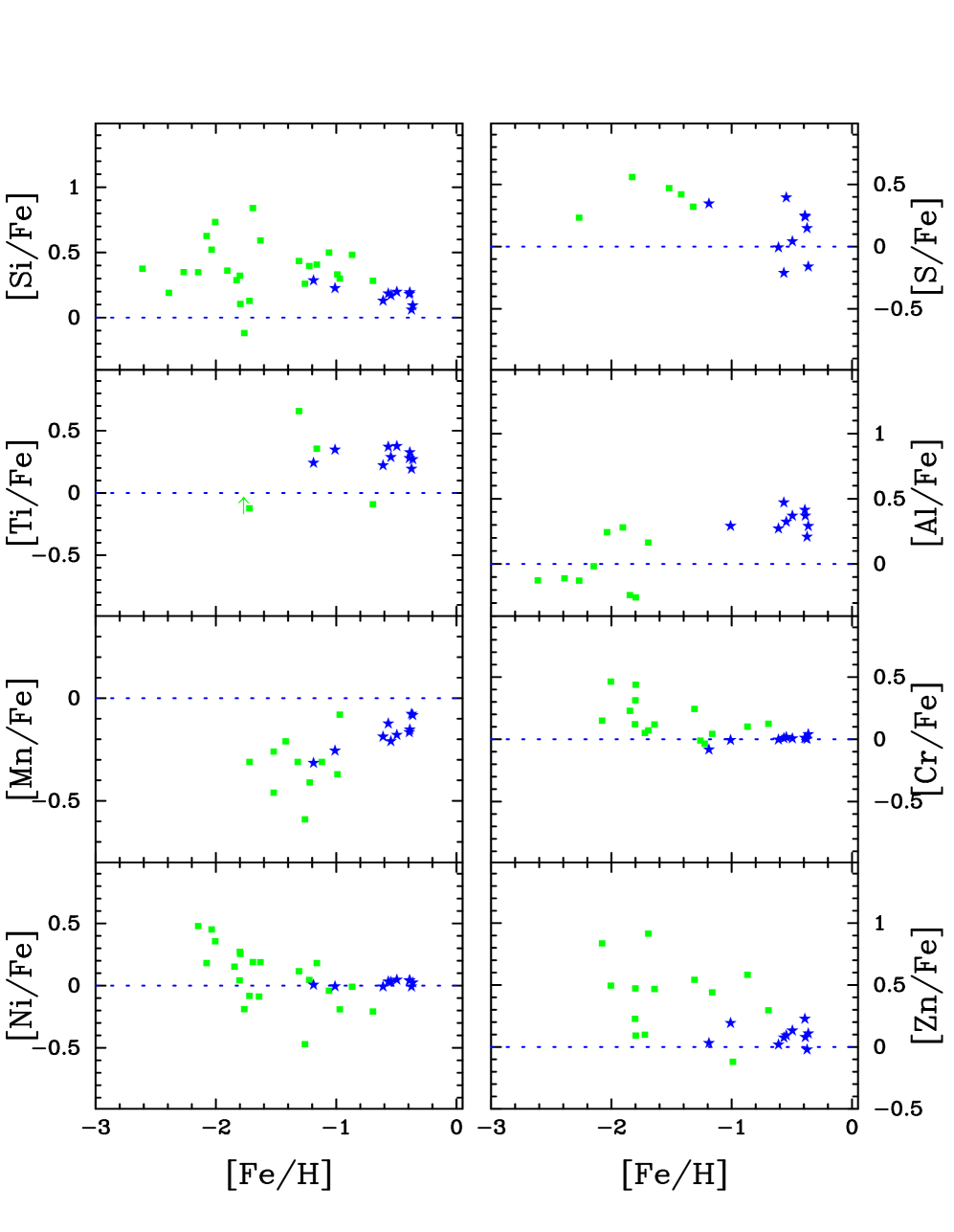
The prospect of nucleosynthetically enhanced Zn/Fe may actually be a welcome sight to the interpretations of the damped Ly$\alpha$ abundance patterns. The current controversy regarding the abundance patterns is the following (see Prochaska & Wolfe 1999 for a more detailed discussion). Figure 26 plots the abundance patterns for a compilation of damped Ly$\alpha$ systems (Lu et al., 1996; Prochaska & Wolfe, 1999) with a range of metallicity. When a stellar abundance researcher examines the plot, s/he sees a classic example of halo abundances with enhanced $\alpha$-elements, deficient Mn and unpeculiar Ni, Cr and Al. The overabundance of Zn relative to Fe would be puzzling yet the overall implication of Type II SN enriched gas would be clear. In fact, one might go so far as to claim that the figure depicts a natural evolutionary sequence in the abundances from the damped systems to the thick disk stars. In contrast, if an expert in the interstellar medium studies the figure, s/he would identify a warm, halo gas dust-depletion pattern to explain the enhanced Si, Zn, and S. This interpretation is consistent with the Ni, Cr, and Al abundances, too, but fails to account for the Mn trend or the two systems with enhanced Ti as neither underabundant Mn nor enhanced Ti is observed in dust depleted gas in the ISM, SMC, or LMC (Savage and Sembach, 1996; Welty et al., 1997, 1999). The difficulty in interpreting the damped Ly$\alpha$ abundance patterns, therefore, has been that two explanations exist which account for the majority of the observations but not all. Because the two interpretations are degenerate in the observed elements, it may even be possible to allow for both Type II SN $\alpha$-enrichment and a dust depletion pattern (although the S/Fe ratio may set an upper limit to the combination; Prochaska & Wolfe 1999).

The implications of a Type II SN enrichment pattern for the damped Ly$\alpha$ abundances are reasonable. These systems have low metallicity and presumably young ages and one would expect them to have been enriched primarily by Type II SN. The difficulty remains, however, in explaining the large Zn/Fe enhancements. On the other hand, if one adopts the ISM perspective then the underlying nucleosynthetic pattern must more closely resemble a Type Ia SN yield (Vladilo, 1998). The implications for this scenario are troubling. First, we know that a significant number of stellar systems exhibit enhanced $\alpha$-elements (e.g. McWilliam, 1997; Trager et al., 2000). If the damped Ly$\alpha$ systems do not contain the gas which gave rise to these systems, then where is that gas? We reemphasize that the damped systems dominate the neutral hydrogen gas content of the universe at all observed epochs ($z=0-4.5$), i.e., that gas which is most likely responsible for star formation. Second, if the gas in the damped systems has been significantly enriched by Type Ia SN, then the stars which polluted these systems must have formed $\approx 1$ Gyr prior to the observed epoch. For a damped system at $z_{abs}\approx 3$, this implies a formation epoch which quickly approaches the Big Bang! For these reasons it is difficult to accept a pure dust depletion explanation for Zn/Fe.

Now consider that Zn/Fe may be enhanced in metal-poor stars and therefore presumably in the metal-poor damped Ly$\alpha$ systems. In this case, a scenario with both dust depletion and Type II SN enhancement is valid, if not favored. While one must introduce dust to account for some of the observed Zn/Fe overabundance, there could still be an underlying Type II SN pattern. The exact level of $\alpha$-enhancement would depend on the dust depletion pattern one assumes, particularly for Si. Dust-corrected enhancements of [Si/Fe] $\approx+0.2$ dex are viable and even enhancements of +0.3 dex are conceivable. Unfortunately, there will always be uncertainties in interpreting Si owing to the exact depletion pattern one adopts. Oxygen would be an ideal prospect for removing this degeneracy if not for the difficulties in measuring O in the damped Ly$\alpha$ systems (Prochaska, 2000).

Figure 27: Solar-corrected [S/Zn] ratios vs. [Fe/H] metallicity for the 9 thick disk stars with S measurements. All of the data points scatter around the solar meteoritic ratio.

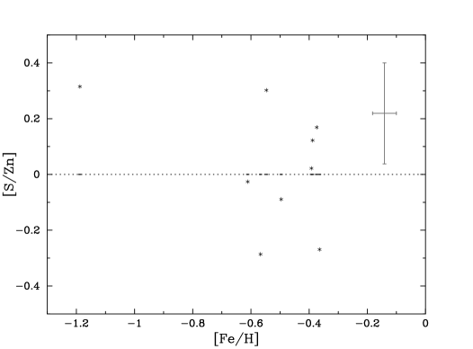
As a final point regarding the damped Ly$\alpha$ systems, consider the S/Zn ratio observed for the thick disk stars. In several recent studies on the damped systems, researchers have suggested that the S/Zn ratio may provide the best indication of nucleosynthesis in these systems (Centurion et al., 2000). The argument follows from the fact that neither S nor Zn are significantly affected by dust depletion and S is expected to be a Type II SN tracer while Zn is a surrogate for Fe. In Figure 27, we plot the [S/Zn] measurements for the 9 thick disk stars with a sulfur measurement. Recall that the sulfur abundances are very sensitive to the assumed $T_{eff}$ values and are based on weak, single line measurements, i.e., the ${\epsilon({\rm S})}$ values are very uncertain. This uncertainty is somewhat tempered by the fact that the Zn I lines have a reasonably significant dependence on $T_{eff}$ such that S/Zn is less affected by errors in $T_{eff}$ than S/Fe. Examining Figure 27 one notes that the [S/Zn] values suggest no significant enhancement in these stars ([S/Zn] = $0.03\pm 0.08$) even though the $\alpha$-elements Ca, Ti, Mg, O, and Si are all enhanced relative to Fe. This result is due to the fact that we find only a mild S/Fe enhancement in the thick disk stars (in contradiction with the observations of Francois 1988) and the observed Zn/Fe enhancement. Of course, it would be most informative to repeat this analysis at metallicities more representative of the damped Ly$\alpha$ systems. Nonetheless, the results suggest that [S/Zn] is not a reliable indicator of nucleosynthesis. In fact, our observations may even help to explain the puzzling sub-solar S/Zn ratios observed by Centurion et al. (2000) in a few damped systems.

6.5 Concluding Summary

We have presented a detailed chemical abundance analysis of 10 kinematically selected thick disk stars with metallicity ranging from $-1.2$ to $-0.4$ dex. The majority of [X/Fe] ratios for the elements studied exhibit significant ($>0.1$ dex) departures from the solar abundance. These include (i) overabundances for all of the $\alpha$-elements except S; (ii) enhancements above solar for the light elements Na and Al; (iii) overabundances of the iron-peak elements Sc, Co, Zn, and V and deficient Mn; (iv) significantly enhanced Eu. For S, Ni, Cr, Cu, Ba, and Y we find essentially solar abundances relative to Fe.

We compared our results with abundance studies of the halo, bulge, and thin disk taken from the literature. These comparisons reveal that in the majority of cases the thick disk stars exhibit X/Fe values distinct from the thin disk. In particular, O, Ca, Mg, Ti, Eu, Al, V, and Co all show enhancements in the thick disk well in excess of those found in the majority of thin disk stars with comparable [Fe/H] metallicity. We argure, therefore, that the thick disk has a distinct chemical history from the thin disk. In general, the thick disk abundances either match or at low [Fe/H] tend toward the patterns observed for halo stars with [Fe/H]$~{}>-1.5$. Most impressive, however, is the excellent agreement between the thick disk and metal-poor bulge star abundance patterns. With the possible exception of Si, the chemical histories of these two stellar populations appear remarkably similar.

Unlike previous elemental abundance studies of the thick disk (Gratton et al., 2000; Fuhrmann, 1998), we find tentative evidence that several $\alpha$-elements (O,Si,Ca) show trends of declining enhancements with increasing [Fe/H]. If these trends are interpreted as evidence for the onset of Type Ia SN (we caution that this is not the only viable explanation), then the thick disk formed over the course of $\gtrsim 1$ Gyr. Because this conclusion has significant impact on formation scenarios for the thick disk, future efforts to confirm the $\alpha$-element trends and investigate other explanations are essential.

We discussed the implications of our observations on the leading formation models of the thick disk. The differences between thick and thin disk abundance patterns imply that the thick disk formed prior to the thin disk and that there exists a significant delay between its formation and that of the thin disk. We argued that if the formation time of the thick disk is $\sim 1$ Gyr then most dissipational collapse models are ruled-out. On the other hand, the clumpy region model of Noguchi (1998) and the merger scenarios (e.g. Quinn et al., 1993) are viable scenarios, although none of these studies considered the formation of the thin disk in a self-consistent manner.

The excellent agreement between the thick disk and the metal-poor bulge abundance patterns provides a strong argument that the two populations shared a common gas reservoir and formation epoch. A conncetion between the two populations has previously been suggested through imaging studies of edge-on spirals (Burstein, 1979) and can be explained by several of the formation scenarios (Jones & Wyse, 1983; Noguchi, 1998). Our observations tighten the association between the two populations, hinting they are intimate from the onset of their formation.

In the final sections, we discussed implications of our analysis on nucleosynthesis in the early universe and interpretations of the damped Ly$\alpha$ abundance patterns. In terms of nucleosynthesis, the conflicting $\alpha$-element trends of Mg, O, Si, Ti, and Ca present a challenge to our current understanding of nucleosynthetic production in Type Ia and Type II SN. We also noted that the Sc, V, Co, and Zn overabundances hint at an overproduction through an enhanced $\alpha$-rich freeze-out process. For the damped Ly$\alpha$ systems, we described the implications of enhanced Zn/Fe in the thick disk stars. In particular, this enhancement allows for interpretations of the damped Ly$\alpha$ abundance patterns which include a combination of dust depletion and Type II SN enrichment patterns. Finally, we noted that the S/Zn ratio is not a good nucleosynthetic indicator.

Our future observational efforts will include obtaining additional spectra of kinematically selected thick disk stars. In particular, we will further investigate the trends of O, Si, and Ca by increasing the sample of thick disk stars with [Fe/H] $\approx-1$ and by adjusting our setups to include the O I [6300] forbidden transition. We also intend to observe thick disk stars at greater radial distances to examine radial dependencies of the abundance trends. To minimize potential systematic errors of comparing our results against abundance studies taken from the literature, we will observe a significant sample of halo stars with [Fe/H] $\approx-1$, thin disk stars with [Fe/H] $\approx-0.5$, and metal-poor bulge stars. The results presented in this paper demonstrate that these stellar populations offer remarkable insight into the Galactic formation history.

Appendix A Stellar Gravity

In those cases where there are Hipparcos parallax measurements, we calculated the stellar gravity according to the following equations.

$$\log(g/g_{\odot})=\log(L/L_{\odot})+\log(M/M_{\odot})+4\log(T/T_{\odot})$$ (A1)

by assuming the following mass relation for these main sequence stars,

$$\log(M/M_{\odot})=0.48-0.105M_{bol}\;\;\;,$$ (A2)

and

$$\log(L/L_{\odot})=-(M_{bol}-4.64)/2.5\;\;\;.$$ (A3)

To estimate the bolometric correction ($BC\equiv M_{V}-M_{bol}$), we interpolated between the tabulated values of Alonso et al. (1995). Given the uncertainties in the parallax and $BC$ values, the error in $\log(g/g_{\odot})$ from this approach is $\approx 0.1$ dex.

Appendix B Hyperfine Splitting

The coupling of the nuclear angular momentum I with the angular momentum of the outer electrons J is known as the hyperfine interaction. These interactions lead to the splitting of absorption lines by typically $1-10$mÅ and can have the effect of de-saturating strong features. As such, it is important to account for hyperfine splitting in order to accurately measure elemental abundances.

Analogous to spin-orbit coupling, one can define the vector sum of the angular momenta as F which has quantum numbers ranging from $|I-J|$ to $|I+J|$. The number of energy states is $2J+1$ when $I\geq J$ and $2I+1$ for $J\leq I$. The allowed transitions must satisfy the Wigner-Eckart theorem, namely $\Delta F=0,\pm 1$ with $0\to 0$ forbidden. While one could calculate the wavelength splittings from first principals, it is usually more accurate to determine them empirically. The energy splitting for a given energy level is typically represented as:

$$\Delta E={1\over 2}AK+B\frac{\frac{3}{4}K(K+1)-J(J+1)\,I(I+1)}{2I(2I-1)(2J-1)}$$ (B1)

where

$$K\equiv F(F+1)-I(I+1)-J(J+1)\;\;\;.$$ (B2)

By determining the $A$ and $B$ constants empirically from very high resolution laboratory experiments for both the upper and lower energy levels, one can calculate the wavelength shifts of hyperfine lines to the precision required for stellar spectroscopy. Kurucz (1999) has compiled the most accurate $A$ and $B$ constants from the literature and calculated the hyperfine lines for nearly all of the absorption lines identified in our spectra. With the exception of Ba (for which we adopt the values provided by McWilliam 1998), we take the values presented by Kurucz.

To calculate the relative line strength $\eta$ of each hyperfine line, one can adopt the Russell-Saunders terms (Condon & Shortly, 1935). In the case where J = J^′ the following equations apply:

$$\eta =\frac{(2F+1)(F(F+1)-I(I+1)+J(J+1))^{2}}{4F(F+1)}\quad\quad\quad[F=F^{\prime}]$$ (B3)

$$=\frac{(F-I+J)(F+I-J)(I+J+F+1)(I+J+1-F)}{4F}\quad[F>F^{\prime}]$$ (B4)

$$=\frac{(F-I+J+1)(F+I-J+1)(I+J+F+2)(I+J-F)}{4(F+1)}\quad[F<F^{\prime}]$$ (B5)

If J is greater than J^′ then,

$$\eta =\frac{(2F+1)(F+J-I)(F+I-J+1)(F+I+J+1)(I+J-F)}{4F(F+1)}\quad[F=F^{\prime}]$$ (B6)

$$=\frac{(F+I-J+1)(I+J-F)(F+I-J+2)(I+J-1-F)}{4(F+1)}\quad[F<F^{\prime}]$$ (B7)

$$=\frac{(F-I+J-1)(F+J-I)(F+I+J+1)(I+J+F)}{4F}\quad[F>F^{\prime}]$$ (B8)

Finally, if J is less than J^′:

$$\eta =\frac{(2F+1)(F+J^{\prime}-I)(L+I-J^{\prime}+1)(F+I+J^{\prime}+1)(I+J^{\prime}-F)}{4F(F+1))}\quad[F=F^{\prime}]$$ (B9)

$$=\frac{(F^{\prime}+I-J^{\prime}+1)(I+J^{\prime}-F^{\prime})(F^{\prime}+I-J^{\prime}+2)(I+J^{\prime}-1-F^{\prime})}{4(F^{\prime}+1)}\quad[F<F^{\prime}]$$ (B10)

$$=\frac{(F^{\prime}-I+J^{\prime}-1)(F^{\prime}+J^{\prime}-I)(F^{\prime}+I+J^{\prime}+1)(I+J^{\prime}+F^{\prime})}{4F^{\prime}}\quad[F>F^{\prime}]$$ (B11)

We then normalize the relative line strengths to give the total $\log gf$ value listed in Table 3. We present the actual values that we have adopted in Table 11 in the event that the Kurucz table is updated after publication.

Table 11: HFS TABLES

Ion	$\lambda$ (Å)	EP (eV)	$\log gf$
Sc II	4670.400	1.357	$-1.182$
Sc II	4670.403	1.357	$-1.353$
Sc II	4670.405	1.357	$-1.560$
Sc II	4670.408	1.357	$-1.831$
Sc II	4670.409	1.357	$-1.922$
Sc II	4670.410	1.357	$-2.249$

References

- Abia & Rebolo (1989) Abia, C. & Rebolo, R. 1989, ApJ, 347, 186
- Allen et al. (1991) Allen, C., Poveda, A., & Schuster, W.J. 1991, A&A, 244, 280
- Alonso et al. (1995) Alonso, A., Arribas, S., & Martinez-Roger, C. 1995, A&A, 297, 197
- Alonso et al. (1996a) Alonso, A., Arribas, S., & Martinez-Roger, C. 1996, A&AS, 117, 227
- Alonso et al. (1996b) Alonso, A., Arribas, S., & Martinez-Roger, C. 1996, A&A, 873, 890
- Bachall & Soneira (1984) Bachall, J.N. & Soneira, R.M. 1984, ApJS, 55, 67
- Bard et al. (1991) Bard, A., Kock, A., & Kock, M. 1991, A&A, 248, 315
- Bard & Kock (1994) Bard, A. & Kock, M. 1994, A&A, 282, 1014
- Baumuller & Gehren (1997) Baumuller, D. & Gehren, T. 1997, A&A, 325, 1088
- Baumuller et al. (1998) Baumuller, D., Butler, K., & Gehren, T. 1998, A&A, 338, 637
- Becker et al. (1980) Becker, U., Zimmermann, P. & Holweger, H. 1980, Geochim. Cosmochim. Acta, 44, 2145
- Beers & Sommer-Larsen (1995) Beers, T. C., & Sommer-Larsen, J. 1995, ApJS, 96, 175
- Beveridge & Sneden (1994) Beveridge, C.R. & Sneden, C. 1994, AJ, 108, 285
- Bimont & Godefroid (1980) Bimont, E. & Godefroid, M. 1980, A&A, 84, 361
- Bimont et al. (1982) Bimont, E., Karner, C., Meyer, G., Trager, F., & zu Putlitz, G. 1982, A&A, 107, 166
- Bimont et al. (1991) Bimont, E., Baudoux, M., Kurucz, R.L., Ansbacher, W., & Pinnington, E.H. 1991, A&A, 249, 539
- Bi Bimont, E., Hibbert, A., Godefroid, M., & Vaeck, N. 1993, ApJ, 412, 431
- Bizzarri et al. (1993) Bizzarri, A., Huber, M.C.E., Noels, A., Grevesse, N., Bereson, S.D., Tsekeris, P., & Lawler, J.E. 1993, A&A, 273, 707
- Blackwell et al. (1976) Blackwell, D.E., Ibbetson, P.A., Petford, A.D., & Willis, R.B. 1976, MNRAS, 177, 219
- Blackwell et al. (1979a) Blackwell, D.E., Ibbetson, P.A., Petford, A.D., & Shallis, M.J. 1979a, MNRAS, 186, 633
- Blackwell et al. (1979b) Blackwell, D.E., Ibbetson, P.A., Petford, A.D., & Shallis, M.J. 1979a, MNRAS, 186, 657
- Blackwell et al. (1980) Blackwell, D.E., Ibbetson, P.A., Petford, A.D., Shallis, M.J., & Simmons, G.J. 1980, MNRAS, 191, 445
- Blackwell et al. (1982a) Blackwell, D.E., Petford, A.D., Shallis, M.J., & Leggett, S. 1982a, MNRAS, 199, 21
- Blackwell et al. (1982b) Blackwell, D.E., Ibbetson, P.A., Petford, A.D., & Shallis, M.J. 1982b, MNRAS, 199, 43
- Blackwell et al. (1982c) Blackwell, D.E., Ibbetson, P.A., Petford, A.D., & Simmons, G.J. 1982c, MNRAS, 201, 595
- Blackwell et al. (1982d) Blackwell, D.E., Menon, P.A., Petford, A.D., & Shallis, M.J. 1982d, MNRAS, 201, 611
- Blackwell et al. (1983) Blackwell, D.E., Menon, & P.A., Petford, A.D. 1983, MNRAS, 204, 883
- Blackwell et al. (1984) Blackwell, D.E., Menon, & P.A., Petford, A.D. 1984, MNRAS, 207, 533
- Blackwell et al. (1986a) Blackwell, D.E., Booth, A.J., Menon, S.L.R., & Petford, A.D. 1986a, MNRAS, 220, 289
- Blackwell et al. (1986b) Blackwell, D.E., Booth, A.J., Menon, S.L.R., & Petford, A.D. 1986b, MNRAS, 220, 303
- Blackwell et al. (1986c) Blackwell, D.E., Booth, A.J., Haddock, D.J., Petford, A.D., & Leggett, S.K. 1986c, MNRAS, 220, 549
- Blackwell et al. (1995a) Blackwell, D.E., Lynas-Gray, A.E., & Smith, G. 1995, A&A, 296, 217
- Blackwell et al. (1995b) Blackwell, D.E., Smith, G., & Lynas-Gray, A.E. 1995, A&A, 303 575
- Booth et al. (1984a) Booth, A.J., Blackwell, D.E., Petford, A.D., & Shallis, M.J., 1984a, MNRAS, 208, 147
- Booth et al. (1984b) Booth, A.J., Blackwell, D.E., & Shallis, M.J., 1984b, MNRAS, 209, 77
- Brown & Wallerstein (1992) Brown, J.A. & Wallerstein, G. 1992, AJ, 104, 1818
- Burstein (1979) Burstein, D. 1979, ApJ, 234, 829
- Butler & Zeippen (1991) Butler, K., & Zeaippen, C.J. 1991, J. Physique IV, Colloque, C1, 141
- Buurman et al. (1986) Buurman, E.P, Dnszelmann, A., Hansen, J.E., & Snoek, C. 1986, A&A, 164, 224
- Cardelli & Savage (1995) Cardelli, J.A. and Savage, B.D. 1995, ApJ, 452, 275
- Cardon et al. (1982) Cardon, B.L., Smith, P.L., Scalo, J.M., Testerman, L. & Whaling, W. 1982, ApJ, 260, 395
- Carney et al. (1989) Carney, B.W., Latham, D.W., & Laird, J.B. 1989, AJ, 97, 423
- Carney et al. (1994) Carney, B.W., Latham, D.W., Laird, J.B., & Aguilar, L.A. 1994, AJ, 107, 2240
- Carney et al. (1996) Carney, B.W., Laird, J.B., Latham, D.W., & Aguilar, L.A. 1996, AJ, 112, 668
- Carney et al. (2000) Carney, B. W., Naumov, S., Laird, J. B., Latham, D. W., Andersen, J., and Nördstrom, B. 2000, in preparation
- Carretta & Gratton (1997) Carretta, E. & Gratton, R.G. 1997, A&AS, 121, 95
- Centurion et al. (2000) Centurion, M., Bonifacio, P., Molaro, P., & Vladilo, G. 2000, ApJ, in press, (astro-ph/0001109)
- Chen (1997) Chen, B., 1997, ApJ, 491, 181
- Chen et al. (2000) Chen, Y.Q., Nissen, P.E., Zhao, G., Zhang, H.W., & Benoni, T. 2000, A&A, in press (astro-ph/9912342)
- Chiba & Beers (2000) Chiba, M., & Beers, T. C. 2000, AJ, in press
- Condon & Shortly (1935) Condon, E.U. & Shortly, G.H. 1935, The Theory of Atomic Spectra, (Cambridge University Press: London), p. 238
- Edvardsson et al. (1993) Edvardsson, B., Anderson, J., Gutasfsson, B., Lambert, D.L., Nissen, P.E., and Tompkin, J. 1993, Astronomy and Astrophysics, 275, 101.
- Eggen et al. (1962) Eggen, O.J., Lynden-Bell, D. & Sandage, A. 1962, ApJ, 136, 748
- ESA (1997) ESA 1997, The Hipparcos and Tycho Catalogues, ESA SP-1200
- Francois (1988) Francois, P. 1988, A&A, 195, 226
- Fry & Carney (1997) Fry, A.M. & Carney, B.W. 1997, AJ, 113, 1073
- Fry et al. (1999) Fry, A.M., Morrison, H.L., Harding, P., & Boroson, T.A. 1999, AJ, 118, 1209
- Fuhr et al. (1988) Fuhr, J.R., Martin, G.A., & Wiese, W.L. 1988, J. Phys. Chem. Ref. Data, 17, Suppl. 4
- Fuhrmann et al. (1995) Fuhrmann, K., Axer, M., & Gehren, T. 1995, A&A, 301, 492
- Fuhrmann (1998) Fuhrmann, K. 1998, A&A, 338, 161
- Garz (1973) Garz, T. 1973, A&A, 26, 471
- Gilmore & Reid (1983) Gilmore, G., & Reid, N. 1983, MNRAS, 202, 1025
- Gilmore & Wyse (1985) Gilmore, G., & Wyse, R. F. G. 1985, AJ, 90, 2015
- Gilmore & Wyse (1987) Gilmore, G. & Wyse, R. F. G. 1987, in The Galaxy, ed. G. Gilmore & B. Carswell, p. 247. (Dordrecht: Reidel)
- Gilmore, Wyse & Kuijken (1989) Gilmore, G., Wyse, R. F. G., Kuijken, K. 1989, ARA&A, 27, 555
- Gilmore et al. (1995) Gilmore, G., Wyse, R.F.G., & Jones, J.B. 1995, AJ, 109, 1095
- Gratton & Sneden (1988) Gratton, R.G. & Sneden, C. 1988, A&A, 204, 193
- Gratton (1989) Gratton, R.G. 1989, A&A, 208, 171
- Gratton & Sneden (1991) Gratton, R.G. & Sneden, C. 1991, A&A, 241, 501
- Gratton & Sneden (1994) Gratton, R.G. & Sneden, C. 1994, A&A, 287, 927
- Gratton et al. (1996) Gratton, R.G., Carretta, E.., Matteucii, F., Sneden, C. 1996, in Formation of the Galactic Halo… Inside and Out, H. Morrison and A. Sarajedini eds., ASP Conference Series, 92, p. 307
- Gratton et al. (2000) Gratton, R.G., Carretta, E.., Matteucii, F., Sneden, C. 2000, A&A, in press (astro-ph/0004157)
- Grevesse et al. (1989) Grevesse, N., Blackwell, D.E., & Petford, A.D. 1989, A&A, 208, 157
- Grevesse et al. (1996) Grevesse, N., Noels, A., & Sauval, A.J. 1996, In: Cosmic Abundances, S. Holt and G. Sonneborn (eds.), ASPCS, V. 99, (BookCrafters: San Fransisco), p. 117
- Grevesse & Sauval (1999) Grevesse, N. & Sauval, A.J. 1999, A&A, 347, 348
- Griffin (1968) Griffin, R.F. 1968, A Photometric Atlas of the Spectrum of Arcturus, (University Printing House: Cambridge)
- Gurtovenko & Kostik (1981) Gurtovenko, E.A. & Kostik, R.I. 1981, A&AS, 46, 239
- Hannaford et al. (1982) Hannaford, P., Lowe, R.M., Grevesse, N., Bimont, E., & Whaling, W. 1982, ApJ, 261, 736
- Hannaford & Lowe (1983) Hannaford, P. & Lowe, R.M. 1983, Opt. Engineering, 22, 532
- Hesser et al. (1987) Hesser, J.E., Harris, W.E., VandenBerg, D.A., Allwright, J.W.B., Shott, P., & Stetson, P.B. 1987, PASP, 99, 739
- Heise & Kock (1990) Heise, C. & Kock, M. 1990, A&A, 230, 244
- Helfer et al. (1959) Helfer, H.L., Wallerstein, G., Greenstein, J.L. 1959, ApJ, 129, 700
- Hoffman et al. (1996) Hoffman, R.D. et al. 1996, ApJ, 460, 478
- Holweger & Muller (1974) Holweger, H. & Mller, E.A. 1974, Solar Phys., 39, 19
- Holweger et al. (1995) Holweger, H., Kock, M., & Bard, A. 1995, A&A, 296, 233
- Huang & Carlberg (1997) Huang, S. & Carlberg, R.G. 1997, ApJ, 480, 503
- Jedamzik et al. (1999) Jedamzik, K., Katalinic, V., & Olinto, A. 1999, Phys. Rev. Lett. submitted (astro-ph/9911100)
- Johnson (1999) Johnson, J. 1999, PhD Thesis, UC Santa Cruz
- Jones & Wyse (1983) Jones, B.J.T. & Wyse, R.F.G. 1983, A&A, 120, 165
- Karner et al. (1981) Karner, C., Meyer, G., Trger, F., zu Putlitz, G. 1981, 23rd Liege, CPSU Conf.
- Kappeler et al. (1990) Kappeler, F., Zhao, W.R,. Beer, H., & Ratzel, U. 1990, ApJ, 355, 348
- Kock & Richter (1968) Kock, M. & Richter, J. 1968, Zs. Ap., 69, 180
- Kroll & Kock (1987) Kroll, S. & Kock, M. 1987, A&AS, 67, 225
- Kurucz et al. (1984) Kurucz, R.L., Furenlid, I., Brault, J., & Testerman, L. 1984, Solar Flux Atlas from 296 to 1300 nm (Sunspot, N.M.: National Solar Observatory)
- Kurucz (1988) Kurucz, R.L. 1988, Trans. IAU, XXB, ed. M. McNally, (Dordrecht: Kluwer), p. 168-172
- Kurucz (1999) Kurucz, R.L. 1999, private communication
- Lambert & Luck (1978) Lambert, D.L. & Luck, R.E. 1978, MNRAS, 183,79
- Landolt-Bornstein (1982) Landolt-Bornstein, “Numerical Data and Functional Relationships in Science and Technology”, Group 6, Vol. 2, ed. K.-H. Hellwege, (Springer-Verlag, New York)
- Larson (1976) Larson, R.B. 1976, MNRAS, 176, 31
- Lawler & Dakin (1989) Lawler, J.E. & Dakin, J.T. 1989, J. Opt. Sco. Am. B6, 1457
- Layden (1995a) Layden, A. C. 1995a, AJ, 110, 2288
- Layden (1995b) Layden, A. C. 1995b, AJ, 110, 2312
- Lu et al. (1996) Lu, L., Sargent, W.L.W., Barlow, T.A., Churchill, C.W., & Vogt, S. 1996, ApJS, 107, 475
- Lu et al. (1997) Lu, L., Sargent, W.L.W., & Barlow, T.A. 1997, astro-ph/9711298
- Luck & Bond (1985) Luck, R.E. & Bond, H.E. 1985, ApJ, 292, 559
- Majewski (1992) Majewski, S. R. 1992, ApJS, 78, 87
- Majewski (1993) Majewski, S.R. 1993, ARA&A, 31, 575
- Martin et al. (1988) Martin, G.A., Fuhr, J.R., & Weise, W.L. 1988, J. Phys. Chem. Ref. D, Vol. 17, No. 3
- Martin & Morrison (1998) Martin, J. C., & Morrison, H. L. 1998, AJ, 116, 1724
- May et al. (1974) May, M., Richter, J., & Wichelmann, J. 1974, A&AS, 18, 405
- McWilliam et al. (1992) McWilliam, A., Geisler, D., & Rich, R.M. 1992, PASP, 104, 1193
- McWilliam (1997) McWilliam, A. 1997, ARA&A, 35, 503
- McWilliam (1998) McWilliam, A. 1998, AJ, 115, 1640
- McWilliam & Rich (1994) McWilliam, A. Rich, R.M. 1994, ApJS, 91, 749
- McWilliam et al. (1995a) McWilliam, A., Preston, G.W., Sneden, C., & Searle,L. 1995a, AJ, 109, 2736
- McWilliam et al. (1995b) McWilliam, A., Preston, G.W., Sneden, C., & Searle,L. 1995b, AJ, 109, 2757
- McWilliam & Rich (2000) McWilliam, A. Rich, R.M. 2000, in preparation
- Meylan et al. (1993) Meylan, T., Furenlid, I., Wiggs, M.S., & Kurucz, R.L. 1993, ApJS, 85, 163
- Moity (1983) Moity, J. 1983, A&AS, 52, 37
- Moore et al. (1966) Moore, C.E., Minnaert, G.J., & Houtgast, J. 1966, The Solar Spectrum, 2nd rev., NBS Monograph 61, (Washington D.C.: U.S. Gov Printing Office)
- Morrison et al. (1990) Morrison, H.L., Flynn, C., & Freeman, K.C. 1990, AJ, 100, 1191
- Morrison et al. (1994) Morrison, H. L., Boroson, T.A., & Harding, P. 1994, AJ, 108, 1191
- Morrison et al. (1997) Morrison, H.L., Miller, E.D., Harding, P., Stinebring, D.R., & Boroson, T.A. 1997, AJ, 113, 2061
- Nissen & Schuster (1997) Nissen, P.E. & Schuster, W.J. 1997, A&A, 326, 751
- Nissen et al. (2000) Nissen, P.E., Chen, Y.Q., Schuster, W.J., & Zhao, G. 2000, (astro/ph-9912269)
- Noguchi (1998) Noguchi, M. 1998, Nature, 392, 253
- Norris et al. (1985) Norris, J., Bessell, M.S., & Pickles, A.J. 1985, ApJS, 58, 463
- Norris (1986) Norris, J. 1986, ApJS, 61, 667
- O’Brian et al. (1991) O’Brian, T.R., Wickliffe, M.E., Lawler, J.E., Whaling, W., & Brault, J.W. 1991, J. Opt. Soc. Am. B, 8, 1185
- O’Connell (1958) O’Connell, D.J.K. 1958, in Ricerche Astronomiche, Proceedings of a Conference at Vatican Observatory, ed. D.J.K. O’Connell (New York: Interscience)
- Ojha et al. (1996) Ojha, D. Bienaymé, O., Robin, A. C., Crézé, M., & Mohan, V. 1996, A&A, 311, 456
- Pilachowski et al. (1996) Pilachowski, C.A., Sneden, C., & Kraft, R.P. 1996, AJ, 111, 1689
- Pettini et al. (1994) Pettini, M., Smith, L. J., Hunstead, R. W., and King, D. L. 1994, ApJ, 426, 79
- Prochaska & Wolfe (1997a) Prochaska, J. X. & Wolfe, A. M. 1997, ApJ, 474, 140
- Prochaska & Wolfe (1999) Prochaska, J.X. & Wolfe, A.M., 1999, ApJS, 121, 369
- Prochaska (2000) Prochaska, J.X. 2000, in preparation
- Prochaska & McWilliam (2000) Prochaska, J.X. & McWilliam, A. 2000, submitted
- Quinn et al. (1993) Quinn, P.J., Hernquist, L., & Fullagar, D.P. 1993, ApJ, 403, 74
- Rao & Turnshek (2000) Rao, S.M. & Turnshek, D.A. 2000, ApJ, in press (astro-ph/9909164)
- Ryan & Lambert (1995) Ryan, S., & Lambert, D. L. 1995, AJ, 109, 2068
- Savage and Sembach (1996) Savage, B. D. and Sembach, K. R. 1996, ARA&A, 34, 279
- Savanov et al. (1990) Savanov, I.S., Huovelin, J., & Tuominen, I. 1990, A&AS, 86, 531
- Schnabel et al. (1999) Schnabel, R., Kock, M., & Holweger, H. 1999, A&A, 342, 610
- Sellwood et al. (1998) Sellwood, J. A., Nelson, R.W., & Tremaine, S. 1998, ApJ, 506, 590
- Shetrone (1996) Shetron, M.D. 1996, AJ, 112, 1517
- Smith & Raggett (1981) Smith, G. & Raggett, D. St.J. 1981, J. Phys. B: Atom. Molec. Phys.,
- Sneden & Crocker (1988) Sneden, C. & Crocker, D.A. 1988, ApJ, 335, 406
- Sneden et al. (1991) Sneden, C., Gratton, R.G., & Crocker, D.A. 1991, A & A, 246, 354
- Steffen (1985) Steffen, M. 1985, A&AS, 59, 403
- Storrie-Lombardi and Wolfe (2000) Storrie-Lombardi, L.J. & Wolfe, A.M. 2000, ApJ, submitted
- Timmes et al. (1995) Timmes, F.X., Woosley, S.E. & Weaver, T.A. 1995, ApJS, 98, 617
- Tinsley (1979) Tinsley, B.M. 1979, ApJ, 229, 1046
- Tomkin et al. (1985) Tomkin, J., Lambert, D.L., & Balachandran, S. 1985, ApJ, 290, 289
- Tomkin et al. (1992) Tomkin, J., Lemke,M., Lambert, D.L., & Sneden, C. 1992, AJ, 104, 1568
- Trager et al. (2000) Trager, S.C., Faber, S.M., Worther, G., & Gonzlez, J.J. 2000, AJ, 119, 1645
- Twarog & Anthony-Twarog (1996) Twarog, B. A., & Anthony-Twarog, B. J. 1996, AJ, 111, 220
- van der Kruit & Searle (1981b) van der Kruit, P.C. & Searle, L. 1981, A&A, 95, 116
- Vladilo (1998) Vladilo, G. 1998, ApJ, 493, 583
- Vogt et al. (1994) Vogt, S.S., Allen, S.L., Bigelow, B.C., Bresee, L., Brown, B., et al. 1994, SPIE, 2198, 362
- Wallerstein (1962) Wallerstein, G. 1962, ApJS, 6, 407
- Welty et al. (1997) Welty, D.E., Lauroesch, J.T., Blades, J.C., Hobbs, L.M., & York, D.G. 1997, ApJ, 489, 672
- Welty et al. (1999) Welty, D.E., Frisch, P.C., Sonneborn, G, & York, D.G. 1999, ApJ, 512, 636
- Wiese & Martin (1980) Wiese, W.L. & Martin, G.A. 1980, Wavelengths and Transition Probabilities for Atoms and Atomic Ions, NSRDS-NBS 68 (Washington: NBS)
- Whaling et al. (1985) Whaling, W., Hannaford, P., Lowe, R.M., Biont, & Grevesse, N. 1985, A&A, 153, 109
- Wheeler, Sneden, & Truran (1989) Wheeler, J.C., Sneden, C., & Truran, J.W.Jr. 1989, ARA & A, 27, 279
- Wickliffe & Lawler (1997) Wickliffe, M.E. & Lawler, J.E. 1997, ApJS, 110, 163
- Wolfe et al. (1995) Wolfe, A. M., Lanzetta, K. M., Foltz, C. B., and Chaffee, F. H. 1995, ApJ, 454, 698
- Wolfe & Prochaska (1998) Wolfe, A.M. & Prochaska, J.X. 1998, ApJ, 494, 15L
- Woosley (1986) Woosley, S.E. 1986, in Nucleosynthesis and Chemical Evolution, ed. B. Hauck, A. Maeder, & G. Meyent (Genevea: Swiss. Soc. Astrophys. Astron., Geneva Obs.), 1
- Woosley & Hoffman (1992) Woosley, S.E. & Hoffman, R.D. 1992, ApJ, 395, 202
- Woosley & Weaver (1995) Woosley, S.E. & Weaver, T.A. 1995, ApJS, 101, 181
- Wyse & Gilmore (1995) Wyse, R. F. G., & Gilmore, G. 1995, AJ, 110, 2771
- Zhao & Magain (1990) Zhao, G. & Magain, P. 1990, A&A, 238, 242
- Zhao & Magain (1991) Zhao, G. & Magain, P. 1991, A&A, 244, 425