Solar Oscillations and Convection: II. Excitation of Radial Oscillations

Abstract

Solar $p$-mode oscillations are excited by the work of stochastic, non-adiabatic, pressure fluctuations on the compressive modes. We evaluate the expression for the radial mode excitation rate derived by Nordlund & Stein (2000) using numerical simulations of near surface solar convection. We first apply this expression to the three radial modes of the simulation and obtain good agreement between the predicted excitation rate and the actual mode damping rates as determined from their energies and the widths of their resolved spectral profiles. These radial simulation modes are essentially the same as the solar modes at the resonant frequencies, where the solar modes have a node at the depth of the bottom of the simulation domain. We then apply this expression for the mode excitation rate to the solar modes and obtain excellent agreement with the low $\ell$ damping rates determined from GOLF data. Excitation occurs close to the surface, mainly in the intergranular lanes and near the boundaries of granules (where turbulence and radiative cooling are large). The non-adiabatic pressure fluctuations near the surface are produced by small instantaneous local imbalances between the divergence of the radiative and convective fluxes near the solar surface. Below the surface, the non-adiabatic pressure fluctuations are produced primarily by turbulent pressure fluctuations (Reynolds stresses). The frequency dependence of the mode excitation is due to effects of the mode structure and the pressure fluctuation spectrum. Excitation is small at low frequencies due to mode properties – the mode compression decreases and the mode mass increases at low frequency. Excitation is small at high frequencies due to the pressure fluctuation spectrum – pressure fluctuations become small at high frequencies because they are due to convection which is a long time scale phenomena compared to the dominant $p$-mode periods.

1 Introduction

Two ideas for the source of $p$-mode excitation have been pursued – overstability (as in pulsating stars) and turbulent Reynolds stresses (as in jet noise) (Biermann, 1948; Schwarzschild, 1948; Lighthill, 1952; Stein, 1967, 1968; Crighton, 1975; Ando & Osaki, 1977; Goldreich & Keeley, 1977; Goldreich & Kumar, 1990; Balmforth, 1992; Musielak et al., 1994). We show here that it is the $PdV$ work of stochastic, non-adiabatic pressure fluctuations which is the primary mode excitation mechanism (Stein & Nordlund, 1991; Bogdan et al., 1993; Goldreich et al., 1994). Near the surface, the non-adiabatic gas pressure (i.e. entropy) fluctuations dominate. They are produced by radiative cooling at the solar surface which is not locally and instantaneously exactly balanced by convective heat deposition. Below the surface, non-adiabatic turbulent pressure (Reynolds stress) fluctuations dominate. They are produced by the turbulent convective motions.

In a previous paper (Nordlund & Stein, 2000) we derived an exact expression for the stochastic excitation rate of the radial solar $p$-modes by the $PdV$ work of non-adiabatic gas and turbulent pressure fluctuations on the mode compression. We now use realistic numerical simulations of near surface solar convection (depth about 2.5 Mm) to evaluate this expression (Stein & Nordlund, 1998). Because the largest entropy and pressure fluctuations occur near the solar surface and because modes with frequencies in the 3 – 4 mHz range, where the excitation rate is largest, are confined near the solar surface, these near surface simulations include the primary excitation and damping processes.

2 Mode Excitation: Formalism

The rate of energy input to the modes can be calculated starting with the kinetic energy equation for the modes (Nordlund & Stein, 2000). Neglecting the viscous stresses,

$$\rho{D\over{Dt}}\left({1\over 2}u_{z}^{2}\right) = -{\partial\over{\partial z}}\left[u_{z}\left(P_{g}+P_{t}\right)\right]+\rho u_{z}g$$ (1)

$$+ \left(P_{g}+P_{t}\right){{\partial u_{z}}\over{\partial z}}\ .$$

After integrating this equation over depth, the flux divergence term only gives contributions from the end points and is negligible. The buoyancy term is small because mass is conserved so there is no net mass flux. The last term is the $PdV$ work,

$$W=\int dt\int dz\delta P{{\partial\dot{\xi}}\over{\partial z}}\ .$$ (2)

There are several contributions to this work. The displacement, $\xi$, has contributions from the modes as well as the random convective motions. The pressure, $\delta P$, has coherent contributions from the modes and incoherent contributions from the random convective motions. Both coherent and incoherent contributions can be further divided into adiabatic and non-adiabatic terms. The dominant driving comes from the interaction of the non-adiabatic, incoherent pressure fluctuations,

$$\delta P^{\rm nad}=\left(\delta\ln P-\Gamma_{1}\delta\ln\rho\right)P\ ,$$ (3)

with the coherent mode displacement,

$${{D\ln\rho}\over{Dt}}=-{{\partial\dot{\xi}}\over{\partial z}}\ .$$ (4)

This is a stochastic process, so the pressure fluctuations occur with random phases with respect to the modes. Therefore one must average over all possible relative phases between them. The resulting rate of energy input to the modes is (Nordlund & Stein, 2000)

$${{\Delta\langle E_{\omega}\rangle}\over{\Delta t}}={{\omega^{2}\left|\int_{r}{dr\delta P^{*}_{\omega}{{\partial\xi_{\omega}}\over{\partial z}}}\right|^{2}}\over{8\Delta\nu E_{\omega}}}\ .$$ (5)

Here, $\delta P_{\omega}$ is the time Fourier transform of the non-adiabatic total pressure. $\Delta\nu=$ 1/(total time interval) is the frequency resolution with which $\delta P_{\omega}$ is computed. $\xi_{\omega}$ is the mode displacement eigenfunction, which is typically chosen to be real for an adiabatic mode. In that case, taking the complex conjugate of the pressure is not necessary, but we retain it for generality. The mode energy is

$$E_{\omega}={1\over 2}\omega^{2}\int_{r}dr~{}\rho~{}\xi_{\omega}^{2}\left({r\over R}\right)^{2}=M_{\omega}V^{2}_{\omega}(R)\ .$$ (6)

Here $M_{\omega}$ is the mode mass and $V_{\omega}(R)$ is the mode velocity amplitude at the surface. Eqn 5 is similar to the expression of Goldreich et al. (1994) (eqn. 26), but involves no approximations. Having the numerical simulation data, we can evaluate this expression exactly without having to make approximations in order to evaluate it analytically

3 Simulations

We simulate a small portion of the solar photosphere and the upper layers of the convection zone, a region extending $6\times 6$ Mm horizontally and from the temperature minimum at $-0.5$ Mm down to $2.59$ Mm below the visible surface. We solve the equations of mass, momentum and energy conservation in the form:

$${{\partial\ln\rho}\over{\partial t}} = -{\bf u}\cdot\nabla\ln\rho-\nabla\cdot{\bf u}\ ,$$ (7)

$${{\partial{\bf u}}\over{\partial t}} = -{\bf u}\cdot\nabla{\bf u}+{\bf g}-{P\over\rho}\nabla\ln P+{1\over{\rho}}\nabla\cdot\underline{\underline{\sigma}}\ ,$$ (8)

$${{\partial e}\over{\partial t}} = -{\bf u}\cdot\nabla e-{P\over\rho}\nabla\cdot{\bf u}$$ (9)

$$+Q_{rad}+Q_{visc}\ ,$$

where $\underline{\underline{\sigma}}$ is the viscous stress tensor, $Q_{rad}$ is the radiative heating and $Q_{visc}$ is the viscous dissipation.

We use a non-staggered grid of either $125^{2}$ cells horizontally $\times 82$ cells vertically or $63^{3}$ cells. The spatial derivatives are calculated using third order splines and the time advance is a third order leapfrog scheme (Hyman, 1979; Nordlund & Stein, 1990). The code is stabilized by a hyper-viscosity which removes short wavelength noise without damping the longer wavelengths.

A large fraction of the internal energy is in the form of ionization energy near the solar surface, so we use a realistic equation of state (including the effects of ionization and excitation of hydrogen and other abundant elements and the formation and ionization of $H_{2}$ molecules). The pressure is found by interpolation in a table of $P(\ln\rho,e)$ and its derivatives which is calculated with the Uppsala stellar atmosphere package (Gustafsson et al., 1975).

Radiative energy exchange is critical in determining the structure of the upper convection zone. Near the surface of the sun, the energy flow changes from almost exclusively convective below the surface to radiative above the surface. The interaction between convection and radiation near the solar surface determines what we observe and produces the entropy fluctuations that lead to the buoyancy work which drives the convection and that give rise to the non-adiabatic pressure fluctuations which excite the p-mode oscillations. Hence, the interaction between convection and radiation is crucial for both the diagnostics and the dynamics of convection. Since the top of the convection zone occurs near the level where the continuum optical depth is one, neither the optically thin nor the diffusion approximations give reasonable results. We therefore include 3D, LTE, non-gray radiation transfer in our model.

We simulate only a small region near the solar surface and must therefore impose boundary conditions inside the convectively unstable region. What happens outside our computational domain in principle influences the convective motions inside. However, at the top boundary, the density is very low relative to the rest of the volume and hence whatever happens there has very little influence on the convective motions. At the bottom, the incoming fluid is to a very good approximation isentropic and featureless, and hence carries little information. The unknown influence of external regions should therefore be small. This assertion is indeed confirmed by experiments with boundaries located at different depths.

The horizontal directions are taken to be periodic. In the vertical direction, we have a transmitting boundary at the temperature minimum (Nordlund & Stein, 1990). This is achieved by a larger than normal zone at the top boundary. Across this zone we make the vertical derivative of the density hydrostatic, set the vertical derivative of the velocity zero and hold the internal energy at the top fiducial layer constant in time and space. At the bottom of the computational domain, outgoing fluid goes out with whatever properties it has. For incoming fluid, we adjust the pressure such that the net mass flux through the bottom boundary vanishes. (This ensures that there is no boundary work done on vertical oscillation modes.) The pressure on the bottom boundary thus varies in time but is uniform over the horizontal plane. We damp fluctuations of the horizontal and vertical velocity of the incoming fluid, using a long time constant. Finally, we adjust the density and energy of the incoming fluid, at constant pressure, to fix its entropy (in both space and time).

The ability to do a direct numerical simulation with the wide range of length scales matching the dimensionless parameters – Reynolds number, Rayleigh number and Prandtl number – of the solar convection zone is beyond the speed and memory capabilities of current computers. Thus, our simulations are of the type called “Large Eddy Simulations”. It is, however, possible to resolve the surface thermal boundary layer of the convection zone and this we have done. Indeed, this is required to achieve results that agree quantitatively with solar observations (Stein & Nordlund, 2000).

The picture of convection that has emerged from the simulations is the following: Convection is driven by radiative cooling in the thin thermal boundary layer at the solar surface. It consists of cool, low entropy, filamentary, turbulent, downdrafts that plunge through a warm, entropy neutral, smooth, diverging, laminar upflow. Upflows must diverge as they ascend into lower density layers in order to conserve mass. This divergence smooths out any variations in their properties that might arise. Only a small fraction of the fluid at depth reaches the surface to be cooled and form the cores of the downdrafts. Most fluid turns over within a scale height and is entrained by the downdrafts. These low entropy downflows are the site of most of the buoyancy work that drives the convection. (See Stein & Nordlund (1998) for more details.)

We have made numerous comparisons between the predictions of the simulations and solar observations:

• The depth of the convection zone depends on the opacities that determine the temperature versus pressure (and hence entropy) stratification of the surface layers, the spectral line blocking, the convective efficiency of the superadiabatic layers immediately below the surface that determines the transition to the asymptotic adiabat, and the equation of state that determines the further run of temperature versus pressure through the convection zone. Excellent agreement is obtained between the depth of the convection zone predicted by our numerical simulations and that inferred from helioseismology (Rosenthal et al., 1999).

• The cavity for high frequency modes is enlarged by turbulent pressure support and 3D non-linear opacity effects which increase the average temperature required to produce a given effective temperature in an inhomogeneous compared to a homogeneous atmosphere. The $p$-mode eigenfrequencies calculated from the mean simulation atmosphere are significantly closer to the observed mode frequencies than those for standard spherically symmetric, mixing length models (Rosenthal et al., 1998, 1999).

• The simulation granulation size spectrum and the distribution of emergent intensities, when smoothed by the point spread function appropriate for the Swedish Vacuum Solar Telescope on La Palma (which produces the best solar images available today), closely match the observations (Stein & Nordlund, 1998).

• The width of photospheric iron lines (whose thermal speed is small) is a signature of the convective velocities. The net Doppler blue shift and asymmetry of spectral lines is a signature of the correlation between velocity and temperature fluctuations. Both these signatures agree closely with observations (Asplund et al., 2000).

This gives us confidence that the simulations are properly modeling the crucial properties of near surface solar convection.

4 Mode Excitation: Simulation

Three radial modes exist in our simulation and we first apply eqn (5) to these modes and compare the rate of work on the modes it predicts with the actual excitation rate $dE_{\omega}/dt=\Gamma E_{\omega}$ determined from the mode’s energies and widths in the simulation. The modes can be clearly seen in the spectrum of the horizontally averaged, depth integrated kinetic energy (fig 1). Their properties are given in table 1. The lowest mode (with no zero crossings inside the computational domain) has a frequency of 2.57 mHz and a FWHM of 19 $\mu$Hz. Hence a simulation significantly longer than 14.5 hrs is required to resolve this mode. We use a simulation of 43 hours, with a spatial resolution of $63^{3}$. Snapshots were saved at 30 s intervals.

Figure 1: Kinetic energy, horizontally averaged and integrated over depth. Three radial modes are clearly visible. Least squares, Lorentzian, fits to the modes and linear fits to the background noise are superimposed.

Table 1: Mode Properties

$\nu$	$\Delta\nu$	$E_{\omega}$	Q	$\Gamma$	dE/dt
(mHz)	($\mu$Hz)	(ergs)		(s-1)	( erg s-1)
2.57	19.0	3.4 $\!\times\!$ 1026	135	1.2 $\!\times\!$ 10-4	4.3 $\!\times\!$ 1022
3.88	133	2.6 $\!\times\!$ 1025	29	8.4 $\!\times\!$ 10-4	2.2 $\!\times\!$ 1022
5.58	438	2.2 $\!\times\!$ 1024	13	2.7 $\!\times\!$ 10-3	6.1 $\!\times\!$ 1021

The eigenfunctions of the velocity are calculated by taking the time Fourier transform of the velocity. To get the real eigenmode, the transform of the velocity at the frequency of the mode is divided by its most common phase among all depths. To reduce the noise, we average the result over a frequency band, approximately equal to the FWHM of the mode, centered on the mode. The eigenfunctions are essentially the same as the solar model modes of Christensen-Dalsgaard using his spherically symmetric model S (Christensen-Dalsgaard et al., 1996) at the mode frequencies (fig 2), when the modes are normalized by the square root of the mode energy, or which is equivalent by their amplitude at the surface. Hence, we choose to use the solar model eigenfunctions, because they are much denser (35 radial modes below the acoustic cutoff frequency instead of three) and because they are slightly smoother.

Figure 2: Velocity eigenmodes of the simulation compared with those of a solar model (model S of Christensen-Dalsgaard et al., 1996). The modes are normalize by the square root of their energy (eqn 6). The solar modes that have nodes at the bottom of the simulation domain closely match the simulation modes. The simulation $p_{1}$ mode corresponds to the solar $p_{16}$ mode and the simulation $p_{2}$ mode corresponds to the solar $p_{26}$ mode. The simulation $p_{3}$ mode lies above the acoustic cutoff frequency.

Another way of looking at the modes is via their kinetic energy. Figure 3 is an image of the logarithm of the kinetic energy as a function of depth and frequency. The three modes of the computational domain are clearly seen. Notice also that there is a continuous pattern of nodes and antinodes, with the nodes descending in depth as the frequency increases and new nodes starting at the surface. This pattern extends even into the propagating region above the acoustic cutoff frequency of about 5.3 mHz.

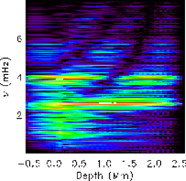
Figure 3: Logarithm of kinetic energy as a function of frequency and depth. The three resonant modes of the simulation stand out as maxima in the kinetic energy. A regular, continuous pattern of nodes and antinodes in the kinetic energy exists both at the resonant modes and between them.

The actual mode energy decay rate of the simulation modes, which on average is equal to their excitation rate, is obtained by multiplying the energy of each mode by its decay rate $\Gamma=2\pi\Delta\nu_{\rm FWHM}$, which is its radian line width and is obtained from the fit to the modes (fig 1).

The total mode energy is the sum of the mode energies minus a fit to the background over the frequency range where the modes are significantly above the background multiplied by the area (36 Mm²) of the simulation domain (fig 1).

Eqn (5) is used to predict the mode excitation rate. The non-adiabatic total (gas + turbulent) pressure fluctuations are calculated directly from the simulation by first averaging the gas pressure, turbulent pressure and density over horizontal planes at each saved snapshot. These are then interpolated to the Lagrangian frame at each time. The non-adiabatic pressure fluctuations are calculated as in eqns A1 and A2. The oscillation modes of the domain are essentially adiabatic and do not affect the non-adiabatic pressure fluctuations as can be seen from its featureless, noisy spectrum (Fig 4). Thus the non-adiabatic pressure work is due primarily to the convection.

Figure 4: Non-adiabatic pressure spectrum at the a depth of 100 km. Note that it is featureless even at the frequencies of the simulation modes. Hence, the non-adiabatic pressure is primarily due to random convective processes.

Figure 5: Mode mass in the simulation domain and the Sun. Mode mass decreases with increasing frequency because higher frequency modes are more concentrated toward the surface than low frequency modes. Because the solar modes extend below the bottom of the simulation domain, they have a larger mode mass. Because the simulation domain is shallow, the mode mass becomes nearly constant at low frequency where the eigenfunctions become nearly constant within the depth of the simulation.

Figure 6: Rate of stochastic energy input to the simulation modes (squares) compared to the predicted excitation rate (small crosses) from the work of non-adiabatic pressure fluctuations on the modes (eqn 5). The solid line is a running boxcar average and the dashed line a two power law fit over the entire frequency range. The excitation rate is larger than the solar case because the mass of the modes in the simulation is less than the mass of the modes in the Sun. The near constancy of simulation mode mass at low frequency leads to a much slower decrease of excitation with decreasing frequency than occurs in the Sun.

The mode compression is calculated from the Christensen-Dalsgaard modes (since these are essentially identical with the simulation modes at the resonant frequencies) normalized by the square root of their energy in the simulation domain. Because the simulation domain is shallow, while, especially at low frequency, the solar modes have substantial amplitude below the computational domain, the mode mass in the computational box is significantly smaller than the actual mode mass of the solar modes (Fig 5).

Figure 7: Rate of stochastic energy input to modes for the entire solar surface (simulation=triangles, observations=squares) from Roca Cortes (1999), based on observed mode velocity amplitudes and line widths from GOLF, for modes with $\ell=0-3$, which are all nearly radial close to the surface. The rate of energy input to the solar modes is smaller than to the simulation modes by the ratio of the mode mass of the solar modes to the mode mass in the simulation domain (fig 5).

Finally, we compare the actual mode energy decay rate with the predicted rate of work by convection on the modes given by eqn (5) in figure 6. The squares are the actual mode energy decay rates for the three resonant modes of the box. The solid line is the running mean of the predicted work and the dashed line is a smooth two power law fit to the predicted work. The agreement is very good, but not perfect. There are significant deviations from the power law fit in the neighborhood of the modes and these are reflected in the actual mode decay rate. This is a phenomena that still remains to be explained. Notice also that the decrease in work toward low frequencies is much slower than for the Sun (Fig 7). The reason is the near constancy of the mode mass within the simulation domain at these low frequencies compared with the steeply rising mode mass with decreasing frequency on the Sun. This application of our excitation rate formula to the modes that are excited in our simulation verifies that the formula is correct and can be applied to the Sun.

5 Mode Excitation: Sun

5.1 Excitation Spectrum

Figure 8: The mode factor in the work integral: ${{\partial\xi_{\omega}}\over{\partial z}}/E_{\omega}^{1/2}$. Excitation decreases at low frequency due to mode behavior, in part because the radial wave vector is approximately $k=\omega^{2}/g$ and in part because the mode mass increases with decreasing frequency (Fig 5).

The excitation rate for solar modes as a function of frequency is shown in Fig. 7. To obtain these results we used the shorter but higher resolution $125^{2}\times 82$ simulation because it has more high frequency power. The magnitude and frequency dependence we find for our 6 Mm square box is very close to the observed values for the entire sun. This means that the pressure fluctuations must be uncorrelated on larger scales, so there is no extra driving contribution.

What produces this frequency dependence? The low frequency behavior is controlled by the nature of the eigenmodes and the high frequency behavior is controlled by the nature of convection. The work integral (Eqn. 5) contains a factor pertaining to the modes: the radial gradient of the mode displacement normalized by the square root of the mode energy (which makes it independent of the mode amplitude). This is small at low frequencies and increases with frequency approximately as $\nu^{3.5}$ (Fig 8). Part of this dependence is due to the radial gradient of the displacement. The mode dispersion relation is $\omega=\surd(gk)$, so $k=\omega^{2}/g$, which accounts for two powers of the frequency. The remainder of the frequency dependence is due to the mode mass, which decreases with increasing frequency because higher frequency modes are more concentrated toward the surface (Fig. 5).

The mode excitation decreases at high frequency because the pressure fluctuation power decreases with increasing frequency roughly as $\nu^{-4}$ (Fig. 9). Convective motions, whose power decreases at small scales and high frequencies, produce the gas and turbulent pressure fluctuations. This then leads to a similar high frequency decline in the pressure spectrum.

Total pressure fluctuations are small at low frequency because the atmosphere is nearly in hydrostatic equilibrium. However, the turbulent pressure fluctuations are largest at low frequency because they are a convective effect and convection is a longer time scale phenomena. Hence, the gas pressure fluctuations must also be large and out of phase with the turbulent pressure fluctuations at low frequency in order to produce small total pressure fluctuations (Fig. 10). The turbulent pressure is small compared to the gas pressure ($\sim$ 15%), but the magnitude of fluctuations are comparable for the gas and turbulent pressures, so they can indeed cancel each other.

Figure 9: Spectrum of pressure fluctuations at a depth of 200 km, smoothed with running boxcar mean. The non-adiabatic gas pressure fluctuations exceed the non-adiabatic turbulent pressure fluctuations by about a factor of four, but they become comparable in the peak driving range at larger depths. The local maxima in the total pressure fluctuations at 2.6, 3.9 and 5.5 mHz are due to the resonant modes in the simulation. The non-adiabatic pressure varies smoothly across these resonant frequencies, indicating it is primarily due to convection. The pressure fluctuation power decreases roughly as $\nu^{-4}$ at high frequency, because it is due due to stochastic convective motions which decrease in power at high frequency.

Figure 10: Correlation of turbulent and gas pressure at the surface. The turbulent pressure is only about 1/6 the magnitude of the gas pressure near the surface but the magnitude of their fluctuations are similar.

Figure 11: Integrand of the work integral, ${\omega^{2}\left|\delta P^{*}_{\omega}{{\partial\xi_{\omega}}\over{\partial z}}\right|^{2}}/{8\Delta\nu E_{\omega}}$, (eqn  5) at 2, 3, 4, and 5 mHz as a function of depth. At frequencies where the driving is large, the integrand is significant only within 500 km of the surface.

5.2 Excitation Location

At what depth does the driving occur? Consider the integrand of the work integral at different frequencies (Figs. 11 and 12). At low frequencies the integrand amplitude is similar over an extended depth range, but it is small. Where the integrand is large, in the region of peak driving around 3-4 mHz, the integrand becomes concentrated very close to the surface and most driving occurs between the surface and 500 km depth. At still higher frequencies the integrand becomes small again and even more concentrated near the surface.

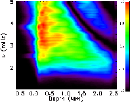
Figure 12: Logarithm (base 10) of the work integrand, ${\omega^{2}\left|\delta P^{*}_{\omega}{{\partial\xi_{\omega}}\over{\partial z}}\right|^{2}}/{8\Delta\nu E_{\omega}}$, (eqn  5) (in units of ergs/cm²/s) as a function of depth and freqency. The work is concentrated close to the surface in the peak excitation range (3 - 4 mHz) and at higher frequencies.

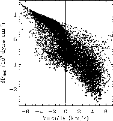
Figure 13: Correlation of non-adiabatic pressure with vertical velocity at the surface. The large negative fluctuations in the non-adiabatic pressure occur where the velocity is positive (downward) in the intergranular lanes.

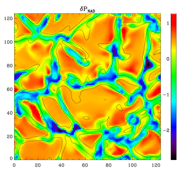
Figure 14: Image of the non-adiabatic total pressure fluctuations at depth 100 km, with the contours of zero surface velocity to outline the granules. The units of the pressure are $10^{3}$ dynes/cm². Large, negative pressure fluctuations occur in the intergranular lanes. Positive pressure fluctuations are half as large and occur inside the granules.

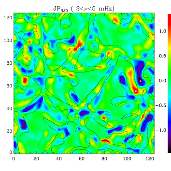
Figure 15: Image of non-adiabatic pressure fluctuations at 100 km depth in the 2 – 5 mHz range, with the contours of zero velocity at the surface to outline the granules. The units of the pressure fluctuations are 10³ dyne cm^-2. In this frequency range, where the driving is maximal, the largest $\delta P_{\rm nad}$ occur at the edges of granules and inside the intergranular lanes.

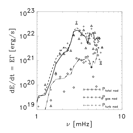
Figure 16: Rate of stochastic energy input to modes for the entire solar surface, showing the individual contributions of the non-adiabatic gas and turbulent pressure to the work of the total non-adiabatic pressure. Most of the driving in the peak driving range comes from the turbulent pressure.

Figure 17: Mode driving at 4 mHz evaluated from the surface to depth z, showing the individual contributions of the non-adiabatic gas and turbulent pressure. Close to the surface the contributions of the two are comparable, but there is little contribution from the gas pressure below 200 km depth, while the turbulent pressure work is significant down to 500 km depth.

Figure 18: Horizontally averaged non-adiabatic pressure at the surface and emergent intensity variation in time. They are tightly correlated indicating that radiative cooling at the surface is the source of the non-adiabatic pressure fluctuations there..

Figure 19: Divergence of the convective and radiative fluxes, at z=100 km, multiplied by ($\Gamma_{3}-1$) compared to the time derivative of the non-adiabatic pressure at the surface. The units are 10³ ergs/cm³/s. The rate of change of non-adiabatic pressure closely follows the divergence of the net flux but has a slightly larger amplitude.

Figure 20: Correlation of the divergence of the convective and radiative fluxes, at z=100 km, multiplied by ($\Gamma_{3}-1$) with the time derivative of the non-adiabatic pressure at the surface. The units are 10³ ergs/cm³/s. The close correlation shows that the slight instantaneous imbalance in the radiative and convective flux divergences is the primary source of non-adiabatic pressure fluctuations.

Where in space does this driving occur? The warm granules have only small non-adiabatic pressure fluctuations. Large, negative fluctuations are concentrated in the downdrafts (Figs. 13, 14).

The maximum mode driving occurs in the frequency range of 3 – 4 mHz, by non-adiabatic pressure fluctuations in the same frequency range. By filtering the time sequence of these fluctuations we see (Fig 15) that in the peak driving range also the driving occurs predominantly in the intergranule lanes and near the edges of granules. The high frequency power near granule edges is due to the motion of the granule boundaries over the one hour time interval on which the filtering was performed. This is, in part, a result of changes in granule size as they evolve. No direct correlation of non-adiabatic pressure fluctuations in the range of 2-5 mHz with velocity is seen. Keep in mind, however, that a correlation plot does not reveal correlations of events that happen in the neighborhood of one another.

5.3 Excitation Source

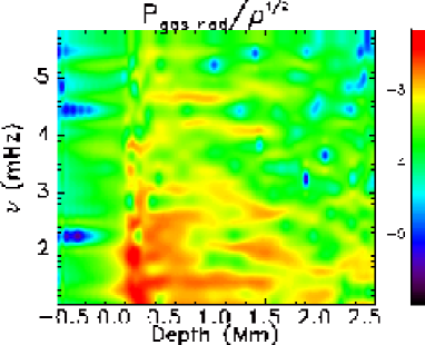
Figure 21: Logarithm of the gas pressure fluctuations scaled by the square root of the density, as a function of depth and frequency. The color scale is identical to the following image of the turbulent pressure fluctuations. With increasing frequency the gas pressure fluctuations become more rapidly concentrated near the surface and decrease more rapidly in strength than the turbulent pressure fluctuations.

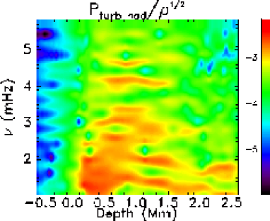
Figure 22: Logarithm of the turbulent pressure fluctuations scaled by the square root of the density, as a function of depth and frequency. The color scale is identical to the preceding image of the gas pressure fluctuations. The turbulent pressure fluctuations extend deeper and decrease less rapidly in magnitude with increasing frequency than the gas pressure fluctuations. As a result, turbulent pressure is the primary source of $p$-mode excitation in the peak driving range of 3-4 mHz.

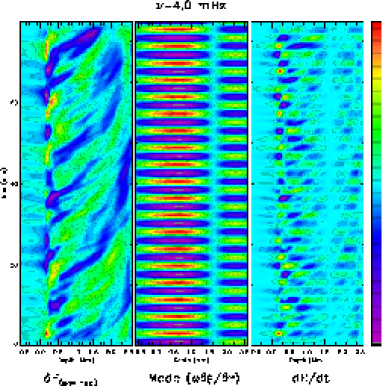
Figure 23: Integrand of the stochastic work integral for non-adiabatic gas pressure only, at 4 mHz, as a function of depth and time (right panel, eqn 5) and the two terms that contribute to it: the horizontally averaged, non-adiabatic gas pressure fluctuations, multiplied by $\langle\rho\rangle^{-1/2}$ (left panel) and the coherent mode density fluctuations multiplied by $\langle\rho\rangle^{1/2}$ (center panel). The non-adiabatic gas pressure fluctuations (left panel) are produced by the imbalance of the convective and radiative energy transport and are largest close to the surface. The color scale goes from maximum negative to maximum positive value for each variable.

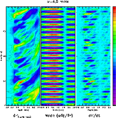
Figure 24: The same as figure 23, but for the non-adiabatic turbulent pressure only. The turbulent pressure fluctuations are more coherent in depth and time than the non-adiabatic gas pressure fluctuations so they produce a more coherent contribution to the work integral.

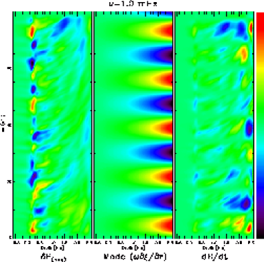
Figure 25: Integrand of the stochastic work integral as a function of depth and time (right panel, eqn 5) and the two terms that contribute to it: the horizontally averaged, non-adiabatic pressure fluctuations, multiplied by $\langle\rho\rangle^{-1/2}$ (left panel) and the coherent mode density fluctuations multiplied by $\langle\rho\rangle^{1/2}$ (center panel). The non-adiabatic pressure fluctuations (left panel) are produced by the imbalance of the convective and radiative energy transport and are largest close to the surface. The color scale goes from maximum negative to maximum positive value for each variable.

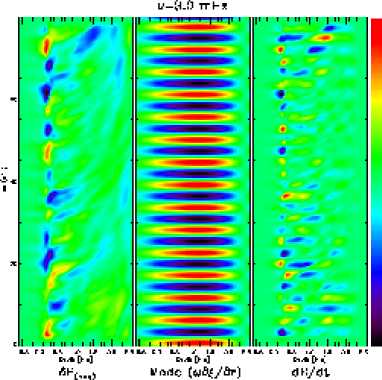
Figure 26: Same as Fig 25, but for $\nu=3$ mHz. At higher frequencies the mode compression (center panel) and hence the work (right panel) becomes more concentrated toward the surface.

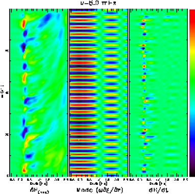
Figure 27: Same as Fig 25, but for $\nu=5$ mHz. The compression and work are even more concentrated toward the surface and the mode has several radial nodes.

What is the source of the non-adiabatic pressure fluctuations? Is it entropy fluctuations or Reynolds stresses? Both play a role, but the primary source of mode driving is turbulent pressure fluctuations (Reynolds stresses) (Fig 16). This is surprising, since the non-adiabatic gas pressure power is larger than the turbulent pressure power near the surface (Fig 9). The non-adiabatic gas and turbulent pressures contribute comparably to the work near the surface, but the contribution of the turbulent pressure extends deeper and provides the dominant contribution to the total work (Fig 17).

The gas pressure fluctuations are significantly larger than the turbulent pressure and have maxima at the frequencies of the three radial modes of the simulation. The non-adiabatic pressure fluctuation power, however, varies smoothly across these frequencies indicating that it is primarily due to stochastic convective processes (Fig 9).

There is a tight correlation between the non-adiabatic pressure fluctuations at the surface and the emergent intensity (Fig 18), which indicates that it is the fluctuating cooling at the surface that is the main source of stochastic mode excitation there. Indeed, the source of entropy fluctuations is the cooling of fluid that approaches optical depth unity (Stein & Nordlund, 1998). This correlated noise is believed to be responsible for the difference in asymmetry of the modal power spectra observed in velocity and intensity (Nigam et al., 1998; Kumar & Basu, 1999). Our discussion in terms of non-adiabatic pressure fluctuations is equivalent to the discussion in terms of entropy fluctuations by Goldreich et al. (1994).

We can use the energy equation to determine the processes producing the non-adiabatic gas pressure fluctuations (Stein & Nordlund, 1991).

$$\delta P_{\rm nad}=\delta P-{{\Gamma_{1}P}\over\rho}\delta\rho=\left({{\partial P}\over{\partial s}}\right)_{\rho}\delta s=(\Gamma_{3}-1)\delta Q\ ,$$ (10)

and

$${{DQ}\over{Dt}}=-{\partial\over{\partial z}}\left(F_{\rm rad}+F_{\rm conv}\right)+\breve{\mathbf{u}}\cdot\nabla P+Q_{\rm diss}\ ,$$ (11)

where $\breve{\mathbf{u}}={\mathbf{u}}-\langle\rho{\mathbf{u}}\rangle/\langle\rho\rangle$ is the convective component of the velocity. The divergence of the radiative and convective fluxes are the dominant terms, but they nearly cancel each other since energy transport shifts from convective to radiative near the surface. It is their slight instantaneous imbalance locally that leads to the non-adiabatic pressure fluctuations (Figs 19 and 20).

The separate contributions of the gas and turbulent pressure to the total non-adiabatic pressure spectrum are shown in figs. 21 and 22, with the same color scale in both. Near the surface, there is clearly more power in the gas pressure. However, in the peak driving range of 3-4 mHz, there is more power in the non-adiabatic turbulent pressure below the surface.

Another reason for the dominance of turbulent pressure in the mode driving is revealed in figs. 23 and 24. The left panels in each show the non-adiabatic gas and turbulent pressures (scaled by $\rho^{-1/2}$) as a function of time and depth. The turbulent pressure varies more slowly with depth and has a longer time scale than the gas pressure. The middle panels show one realization of the mode density or compression (scaled by $\rho^{1/2}$). The right panels show the work integrand, $\delta P_{{\rm nad}\omega}\partial\xi_{\omega}/\partial zE_{\omega}^{-1/2}$. The gas pressure contribution to the integrand is more concentrated at the surface and alternates sign with time and depth more rapidly than the turbulent pressure contribution. The greater coherence of the turbulent pressure allows it to make a greater contribution to the net work.

The very largest pressure perturbations are associated with the sudden initiation of downdrafts and produce waves that propagate up into the chromosphere and steepen into shocks (Skartlien, 1998; Skartlien et al., 2000). These events may correspond to the large individual acoustic events observed by Rimmele et al. (1995) and Goode et al. (1998). They may be the tail of the distribution of the stochastic driving process. A comparison of observed acoustic events and those in the simulation has been made by Goode et al. (1998).

6 Summary

How does this all fit together? Figs 25 – 27 show the time variation of the horizontally averaged non-adiabatic pressure fluctuations, the density (compression) in the modes and the product of the two which is the integrand of the work integral (eqn 5) as a function of depth and time for modes with frequencies 1,3, and 5 mHz.

The dominant contribution to the work comes from the turbulent pressure (Reynolds Stress). Near the surface non-adiabatic gas pressure fluctuations, produced by an instantaneous imbalance between the divergences of the radiative and convective fluxes, also contribute. Their divergence is individually large, but since energy transport switches between convection and radiation in the surface layers, they are nearly equal and opposite. At each instant they do not exactly cancel, which leads to heating and cooling and hence entropy fluctuations. Excitation is small at low frequencies due to mode properties – the mode compression decreases and the mode mass increases at low frequency. In addition, at low frequency the mode amplitude is small near the surface where the non-adiabatic pressure fluctuations are large. (At very low frequencies, driving occurs deeper than the simulation domain.) Excitation is small at high frequencies due to the pressure fluctuation spectrum – pressure fluctuations become small at high frequencies because they are due to convective motions which have a longer time scale than the dominant $p$-mode periods. Large non-adiabatic pressure fluctuations occur primarily in the intergranular lanes (due to turbulence and surface radiative cooling) and near the edges of granules (due to granule expansion and collapse).

Appendix A Evaluation of the Mode Excitation Rate (eqn 5)

The mode excitation rate (eqn 5) can be evaluated in two different ways: in Fourier space and in real space. We describe both methods. The variables that appear in eqn 5 for the mode excitation are the non-adiabatic total pressure fluctuation, the derivative of the mode displacement and the mode energy. These quantities are calculated as follows for both methods of evaluating the excitation.

The non-adiabatic pressure fluctuations are obtained from the simulation results. First the gas pressure, turbulent pressure ($P_{t}=\langle\rho u_{z}^{2}\rangle$) and density are averaged over horizontal planes and saved at 10 s or 30 s intervals. These are then interpolated to the Lagrangian frame, that moves with the vertical (radial oscillation) motions. The Lagrangian frame is determined by calculating the mass column density at each time and interpolating the variables to the time average mass column density. Next, the non-adiabatic total (gas plus turbulent) pressure is calculated from

$$P^{\rm nad}=\left(\ln(P_{\rm gas}+P_{\rm turb})-\Gamma_{1}\ln\rho\right)(P_{\rm gas}+P_{\rm turb})\ .$$ (A1)

Finally, the fluctuation of the non-adiabatic total pressure about its time average,

$$\delta P^{\rm nad}(z,t)=P^{\rm nad}(z,t)-\langle P^{\rm nad}(z,t)\rangle_{t}\ ,$$ (A2)

is determined.

The mode displacement $\xi_{\nu}(z)$ for the radial mode of frequency $\nu$ is obtained from the eigenmode calculations of Christensen-Dalsgaard, using his spherically symmetric model S (Christensen-Dalsgaard et al., 1996). Alternatively, one could extract modes directly from the numerical simulations, using Fourier decomposition. A drawback with this method is, apart from slightly noisier mode structure, that there are only three resonant modes in the shallow simulation box—the 35 radial modes from standard solar models provide much better frequency coverage. As we have shown (fig 2), the modes from the simulation are essentially the same as the solar modes at the resonant frequencies of the computational domain, where the solar modes have a node at the depth of the bottom of the computational domain.

The mode energy is calculated from the displacement according to eqn. 6. The mode displacements are interpolated to the simulation grid at the same total pressure as in the Christensen-Dalsgaard model and the derivative of the displacement is calculated. Since the derivative of the mode displacement always appears normalized by the square root of the mode energy, the mode amplitude normalization cancels.

In Fourier space, the work integral which appears in the energy input rate to the modes (eqn 5) is evaluated by taking the time Fourier transform of the total non-adiabatic pressure fluctuations at each depth, $\delta P^{\rm nad}(z,t)$. For each frequency and depth, this is multiplied by the spatial derivative of the mode displacement at that depth interpolated to the frequencies of the Fourier transform (and normalized by the square root of the mode energy), $\omega(\partial\xi_{\omega}/\partial r)E_{\omega}^{-1/2}$. The spatial dependence of the modes varies slowly and continuously with frequency, so such interpolation is possible. This product is integrated over the depth of the simulation domain for each frequency. The energy input rate to the modes is the square of the absolute value of this work integral, divided by the frequency interval for the Fourier transform, $\Delta\nu$, (which equals multiplying by the time interval of the simulation), multiplied by the area of the simulation (36 ${\rm Mm}^{2}$) and divided by eight (Eqn 5).

In real space, the integrand of the work integral for each frequency, $\nu$, is calculated as the non-adiabatic total pressure fluctuation at each depth and time, $\delta P^{\rm nad}(z,t)$, multiplied by the normalized derivative of the mode displacement for that frequency at each depth, $\omega({\partial\xi_{\omega}(z)}/{\partial z})/E_{\omega}^{1/2}$, multiplied by a phase function $\cos\left(\phi+\omega t\right)$ for each time, $t$, a snapshot was saved in the simulation (10 s or 30 s intervals). For each depth, this is summed over all saved snapshots in the longest interval that is an integral number of mode periods for the given mode frequency $\nu$, and divided by the number of snapshots summed over to get the average value. This integrand is then integrated over depth. This is done for two values of the phase, $\phi=0\ {\rm and}\ \pi/2$ (since the phases between the modes and the pressure fluctuations are random, we average these two orthogonal cases). The value of the integral for each phase is squared and these two values are summed. The energy input rate to the mode at this frequency is this average multiplied by the time interval integrated over (for that frequency), multiplied by the area of the simulation (36 ${\rm Mm}^{2}$), and divided by eight.

References

- Ando & Osaki (1977) Ando, H., Osaki, Y. 1977, PASJ, 29, 221
- Asplund et al. (2000) Asplund, M., Nordlund, Å., Trampedach, R., Allende Prieto, C., Stein, R. F. 2000, Astronomy and Astrophysics (accepted), astro-ph/0005320
- Balmforth (1992) Balmforth, N. J. 1992, MNRAS, 255, 639
- Biermann (1948) Biermann, L. 1948, Z. f. Astrophys., 25, 161
- Bogdan et al. (1993) Bogdan, T. J., Cattaneo, F., Malagoli, A. 1993, ApJ, 407, 316
- Christensen-Dalsgaard et al. (1996) Christensen-Dalsgaard, J., Däppen, W., Ajukov, S. V., Anderson, E. R., Antia, H. M., Basu, S., Baturin, V. A., Berthomieu, G., Chaboyer, B., Chitre, S. M., Cox, A. N., Demarque, P., Donatowicz, J., Dziembowski, W. A., Gabriel, M., Gough, D. O., Guenther, D. B., Guzik, J. A., Harvey, J. W., Hill, F., Houdek, G., Iglesias, C. A., Kosovichev, A. G., Leibacher, J. W., Morel, P., Proffitt, C. R., Provost, J., Reiter, J., Jr., R., J., E., Rogers, F. J., Roxburgh, I. W., Thompson, M. J., Ulrich, R. K. 1996, Science, 272, 1286
- Crighton (1975) Crighton, D. G. 1975, Prog. Aerospace Sci., 16, 31
- Goldreich & Keeley (1977) Goldreich, P., Keeley, D. A. 1977, ApJ, 212, 243
- Goldreich & Kumar (1990) Goldreich, P., Kumar, P. 1990, ApJ, 363, 694
- Goldreich et al. (1994) Goldreich, P., Murray, N., Kumar, P. 1994, ApJ, 424, 466
- Goode et al. (1998) Goode, P. R., Strous, L. H., Rimmele, T. R., Stebbins, R. T. 1998, apjl, 495, L27
- Gustafsson et al. (1975) Gustafsson, B., Bell, R., Eriksson, K., Nordlund, Å. 1975, Astronomy and Astrophysics, 42, 407
- Hyman (1979) Hyman, J. 1979, in R. Vichnevetsky, R. S. Stepleman (eds.), Adv. in Comp. Meth. for PDE’s—III, 313
- Kumar & Basu (1999) Kumar, P., Basu, S. 1999, ApJ, 519, 389
- Lighthill (1952) Lighthill, M. J. 1952, Proc. R. Soc. London, A211, 564
- Musielak et al. (1994) Musielak, Z. E., Rosner, R., Stein, R. F., Ulmschneider, P. 1994, ApJ, 423, 474
- Nigam et al. (1998) Nigam, R., Kosovichev, A. G., Scherrer, P. H., Schou, J. 1998, ApJ, 495, L115
- Nordlund & Stein (1990) Nordlund, Å., Stein, R. F. 1990, Computer Phys. Communications, 59, 119
- Nordlund & Stein (2000) Nordlund, Å., Stein, R. F. 2000, ApJ (accepted), astro-ph/0006336
- Rimmele et al. (1995) Rimmele, T. R., Goode, P. R., Harold, E., Stebbins, R. T. 1995, ApJ, 444, L119
- Roca Cortes et al. (1999) Roca Cortes, T., Montanes, P., Palle, P. L., Perez Hernandez, F., Jimenez, A., Regula, C., the GOLF Team 1999, in A. Gimenez, E. Guinan, B. Montesinos (eds.), Theory and Tests of Convective Energy Transport, Vol. 173 of ASP Conf. Ser., 305
- Rosenthal et al. (1998) Rosenthal, C. S., Christensen-Dalsgaard, J., Kosovichev, A. G., Nordlund, Å., Reiter, J., Rhodes, E. J., J., Schou, J., Stein, R. F., Trampedach, R. 1998, in SOHO 6/GONG 98: Structure and Dynamics of the Interior of the Sun and Sun-like Stars, ESA, p. (521
- Rosenthal et al. (1999) Rosenthal, C. S., Christensen-Dalsgaard, J., Nordlund, Å., Stein, R. F., Trampedach, R. 1999, A&A, 351, 689
- Schwarzschild (1948) Schwarzschild, M. 1948, ApJ, 107, 1
- Skartlien (1998) Skartlien, R. 1998, 3D modeling of solar convection and atmosphere dynamics, PhD Thesis, University of Oslo
- Skartlien et al. (2000) Skartlien, R., Stein, R., Nordlund, Å. 2000, ApJ (accepted)
- Stein (1967) Stein, R. F. 1967, Solar Physics, 2, 385
- Stein (1968) Stein, R. F. 1968, ApJ, 297, 154
- Stein & Nordlund (1991) Stein, R. F., Nordlund, Å. 1991, in D. Gough, J. Toomre (eds.), Challenges to Theories of the Structure of Moderate Mass Stars, Vol. 388 of Lecture Notes in Physics, Springer, Heidelberg, p. 195
- Stein & Nordlund (1998) Stein, R. F., Nordlund, Å. 1998, ApJ, 499, 914
- Stein & Nordlund (2000) Stein, R. F., Nordlund, Å. 2000, Solar Phys., (in press)