Near-infrared and Br$\gamma$ observations of post-AGB stars

Abstract

In this article we report further investigations of the IRAS selected sample of Planetary Nebula (PN) candidates that was presented in Van de Steene & Pottasch (VdSteene93 (1993)). About 20 % of the candidates in that sample have been detected in the radio and/or H$\alpha$ and later confirmed as PNe. Here we investigate the infrared properties of the IRAS sources not confirmed as PNe.

We observed 28 objects in the N-band of which 20 were detected and 5 were resolved, despite adverse weather conditions. We obtained medium resolution Br$\gamma$ spectra and we took high resolution JHKL images of these 20 objects. We critically assessed the identification of the IRAS counterpart in the images and compared our identification with others in the literature. High spatial resolution and a telescope with very accurate pointing are crucial for correct identification of the IRAS counterparts in these crowded fields.

Of sixteen positively identified objects, seven show Br$\gamma$ in absorption. The absorption lines are very narrow in six objects, indicating a low surface gravity. Another six objects show Br$\gamma$ in emission. Two of these also show photospheric absorption lines. All emission line sources have a strong underlying continuum, unlike normal PNe. In another three objects, no clear Br$\gamma$ absorption or emission was visible. The fact that our objects were mostly selected from the region in the IRAS color-color diagram where typically PNe are found, may explain our higher detection rate of emission line objects compared to previous studies, which selected their candidates from a region between AGB and PNe.

The objects showing Br$\gamma$ in emission were re-observed in the radio continuum with the Australia Telescope Compact Array. None of them were detected above a detection limit of 0.55 mJy/beam at 6 cm and 0.7 mJy/beam at 3 cm, while they should have been easily detected if the radio flux was optically thin and Case B recombination was applicable. It is suggested that the Br$\gamma$ emission originates in the post-Asymptotic Giant Branch (post-AGB) wind, and that the central star is not yet hot enough to ionize the AGB shell.

We measured the JHKL magnitudes of the objects and present their infrared spectral energy distributions. They are typical for post-AGB stars according to the scheme of van der Veen et al. (vdVeen89 (1989)). We also constructed various color-color diagrams using the near-infrared and IRAS magnitudes. No distinction can be made between the objects showing Br$\gamma$ in emission, absorption, or a flat spectrum in the near and far-infrared color-color diagrams. The near-infrared color-color diagrams show evidence for a very large range of extinction, which in part is of circumstellar origin. Near-infrared versus far-infrared color-color diagrams show trends that are consistent with the expected evolution of the circumstellar shell. This sample of post-AGB stars show a larger range in color and are generally redder and closer to the galactic plane than the ones known so far.

The properties of most of these objects are fully consistent with the assumption that they are post-AGB stars that have not evolved far enough yet to ionize a significant fraction of their circumstellar material.

1 Introduction

A most intriguing challenge is to understand how Asymptotic Giant Branch (AGB) stars transform their surrounding mass-loss shells in a couple of thousand years into the variety of shapes and sizes observed in Planetary Nebulae (PNe). There are a number of theories currently being investigated. In the generalized interacting stellar wind model, a variety of axisymmetric PN shapes are obtained by the interaction of a very fast central star wind with the progenitor AGB circumstellar envelope (Kwok Kwok82 (1982)), when the latter is denser near the equator than the poles (Frank et al. Frank93 (1993) ). Sahai & Trauger (Sahai98 (1998)) proposed that the primary agent for shaping PNe is not the density contrast, but a high speed collimated outflow of a few 100 km/s. No consensus about the dominant physical process responsible for the shaping of PNe has emerged so far, but there is agreement that they occur during the early AGB-to-PN transition stage. However, details of the rate of evolution, the strength of the stellar wind, and the impact of ionization across the transition phase are very poorly known. In order to test model predictions it is essential to study nebulae from the early post-AGB phase through the very early PN phases. However, post-AGB objects are difficult to find, because this phase is very short and the star is usually obscured by a thick circumstellar dust shell.

One way of identifying new post-AGB stars is through their dust emission. In our search for new obscured PNe and post-AGB stars, we selected candidates from the IRAS Point Source Catalogue based on infrared colors typical of PNe. When we observed these candidates in the radio continuum at 6 cm, on average 20 % of the objects were detected (Van de Steene & Pottasch VdSteene93 (1993), VdSteene95 (1995)). Subsequent optical spectroscopy showed that the PN candidates detected in the radio have emission line spectra typical of PNe (Van de Steene et al. 1996a , 1996b ). However, the question remained: what is the evolutionary status of those IRAS sources with colors typical of PNe, which had no detectable ionization in the radio (i.e. fluxes below 3 mJy)? It is possible that a few large, low surface-brightness PNe have escaped detection. Others of the remaining non-identified PN candidates could be very young and small PNe. Their radio flux would have been below our detection threshold and they wouldn’t be identified in H$\alpha$ due to extinction. However, the true evolutionary status of most objects with IRAS colors typical of PNe has remained unknown.

We have calculated evolutionary tracks for post-AGB stars in the IRAS color-color diagram (van Hoof et al. vHoof97 (1997)). From this study, it became clear that post-AGB objects and PNe could be located in the same region in the IRAS color-color diagram. No other types of objects seem to have typically these particular IRAS colors. We therefore adopted the working hypothesis that the non-detected PN candidates are AGB-to-PN transition objects. The goal of this project is to determine the evolutionary status of these post-AGB candidates, their physical properties, and to relate them to their morphology.

To ensure the identification of the correct counterpart of the IRAS source and obtain accurate positions for follow-up observations, we first imaged the post-AGB candidates in the N-band. In order to investigate whether the sources have some ionization, we obtained Br$\gamma$ spectra. We reobserved the sources showing Br$\gamma$ emission at 3 cm and 6 cm. To confirm the identification, obtain finding charts, and photometry, we took high resolution near-infrared (JHKL) images.

The next section describes the observations. In Section 3 we describe the data reduction and analysis, in Section 4 we discuss the individual objects and in Section 5 we discuss the general results. We give a summary in the last section.

2 Observations

2.1 Imaging

2.1.1 N-band

Table 1: Observation log for the timmi observations. The first column gives the object name, the second column the observation date, the third column the total integration time in seconds, the fourth column gives the IRAS 12-$\mu$m band flux in jansky, and the last column indicates whether the object was detected or not.

Name	Date	I.T.	$S_{12}$	detected
IRAS	dd/mm/yy	s	Jy	yes/no
10256$-$5628	10/05/95	155	4.30	yes
11159$-$5954	10/05/95	466	1.08	yes
11387$-$6113	11/05/95	404	3.56	no
13356$-$6249	10/05/95	155	6.06	yes
13416$-$6243	11/05/95	93	38.8	yes
13428$-$6232	10/05/95	404	21.9	yes
13428$-$6531	10/05/95	466	0.53	no
13529$-$5934	10/05/95	466	1.37	yes
14325$-$6428	10/05/95	218	3.31	yes
14488$-$5405	11/05/95	155	6.59	yes
15066$-$5532	10/05/95	466	1.43	yes
15144$-$5812	11/05/95	218	7.67	yes
15154$-$5258	11/05/95	684	2.25	no
15310$-$6149	11/05/95	404	3.67	no
15544$-$5332	11/05/95	218	4.64	yes
15553$-$5230	10/05/95	155	9.99	yes
16086$-$5255	11/05/95	155	5.70	yes
16115$-$5044	10/05/95	249	10.4	no
16127$-$5021	11/05/95	280	2.90	yes
16130$-$4620	11/05/95	155	4.73	yes
16209$-$4714	11/05/95	404	1.17	no
16279$-$4757	10/05/95	93	43.0	yes
16328$-$4517	11/05/95	280	3.73	yes
16345$-$5001	11/05/95	218	2.45	no
16594$-$4656	10/05/95	93	44.9	yes
17009$-$4154	10/05/95	311	7.44	yes
17088$-$4221	11/05/95	93	42.7	yes
17234$-$4008	10/05/95	839	1.73	no

Mid-infrared images in the N-band were obtained with the Thermal Infrared Multi Mode Instrument (timmi) at the European Southern Observatory 10–12 May 1995. The camera featured a 64 $\times$ 64 element Gallium doped Silicon array with good cosmetic quality and a quantum efficiency of 25 %. We used the N-band filter: $\lambda_{\rm c}$ = 9.70 $\mu$m and $\Delta\lambda$ = 5.10 $\mu$m with a setup yielding a pixel size of 0$\aas@@fstack{\prime\prime}$66, and a FOV of $\approx$ 40″.

For the cancelation of the strong background radiation, timmi is operated in chopping and nodding mode. The chopping frequency is several hertz and nodding is done once or twice per minute. In chopping mode a pair of exposures is obtained: one exposure contains object plus sky and the second exposure, 20″ away, only sky. To obtain the images in nodding mode the telescope was moved by an angle exactly matching the chopper throw on the sky and the observation in chopping mode was repeated. Because this observation is exactly 180 degrees out of phase with the first one, the observed object shows up as a negative measurement. Subtracting both images resulted in a clean image corrected for first and second order effects introduced by the strong and inhomogeneous background radiation. To eliminate erratic pixels, the multiple images of each object were median filtered with a high threshold. Finally the images were Fourier transformed and the midas standard low bandpass Butterworth filter was applied to better reveal the sources.

A log of the observations can be found in Table 1. The weather was poor during both nights. Consequently, only the brighter IRAS sources could be detected, while under favorable weather conditions timmi would be ten times more sensitive than IRAS. All but one of the undetected sources have an IRAS 12-$\mu$m flux below 4 Jy. Six sources having a 12-$\mu$m flux below 4 Jy were detected when the cloud conditions improved temporarily. The other 14 detected sources have a larger IRAS 12-$\mu$m flux. We think that non-detections are due to the cloudy weather rather than faulty IRAS positions or inaccurate telescope pointing.

2.1.2 Near-infrared images

JHKL-band images of the 20 post-AGB candidates detected in the N-band were obtained with caspir at the 2.3-m telescope at Siding Spring Observatory in Australia on 11 and 12 March 1998. The detector is a SBRC CRC463 $256\times 256$ InSb array which is sensitive from approximately 0.9 $\mu$m to 5.5 $\mu$m. The pixel size was 0$\aas@@fstack{\prime\prime}$25 and the total field of view 1′. Each object was observed 60 times for 0.3 s at 12″ north and 12″ south of its nominal position. The objects were observed in order of right ascension: IRAS 10256$-$5628 to 15144$-$5812 on 11 March 1998 and IRAS 15544$-$5332 to 17088$-$4221 on 12 March 1998. Both nights were photometric. Standard stars were observed at the beginning of the observations each night. The seeing was sub-arcsecond.

2.2 Observing the Br$\gamma$ line

Using the improved positions from the timmi images, we obtained infrared spectra with irspec at the NTT at ESO 13 and 14 May 1995.

The spectra are centered at Br$\gamma$ and have a resolution of $\lambda/\Delta\lambda\approx 2000$. The SBRC $62\times 58$ array gives a total wavelength coverage from 2.15 $\mu$m to 2.18 $\mu$m. The resolution in the spatial direction is 2$\aas@@fstack{\prime\prime}$26/pixel. Since the outer edges of the array are vignetted, the total field of view is approximately 1$\aas@@fstack{\prime}$5. The slit width is 2 pixels or 4$\aas@@fstack{\prime\prime}$51. The slit orientation was north-south. First we pointed the telescope to a bright star, and subsequently offset the telescope to the timmi position. The pointing accuracy of the NTT has an rms of about 1″. Subsequently we moved the slit east- and westwards a few arcseconds, to ‘peak-up’ the strongest signal in order to center the object in the slit. The resulting offsets were never larger than 6″.

To subtract the sky emission the beam-switching technique was used. Because all but one (IRAS 13428$-$6232) of the sources are much smaller than 20″, two spectra were taken with the source at different positions on the array, such that when the exposures were subtracted, the spectra did not overlap. For IRAS 13428$-$6232 one integration was taken on source and one on the sky and these images were subsequently subtracted

The weather was very good, and the humidity was around 15 %. Within the accuracy limits of spectro-photometry the night was photometric, even if the conditions slightly deteriorated at the end of the night. Every 30 to 60 min a standard star was observed. A complete log of the observations can be found in Table 2. Note that the observations include four PNe from Van de Steene & Pottasch (VdSteene95 (1995)).

Table 2: Observation log for the irspec observations. The first column gives the object name, the second column the total on-source integration time in seconds, the third column the estimated signal-to-noise ratio, the fourth column the airmass.

Object	I.T.	S/N	Airm.	Comment
10256$-$5628	1200s	170	1.135
11159$-$5954	600s	970	1.172
13356$-$6249	1200s	385	1.292
13416$-$6243	720s	605	1.261
13428$-$6232	900s	135	1.220
13529$-$5934	3240s	32	1.166
14325$-$6428	600s	165	1.226
14488$-$5405	720s	225	1.104
15066$-$5532	720s	130	1.127
15144$-$5812	900s	340	1.163
15544$-$5332	720s	370	1.106
15553$-$5230	1080s	34	1.107
16086$-$5255	1080s	56	1.118
16127$-$5021	1200s	100	1.120
16130$-$4620	1080s	50	1.134
16279$-$4757	360s	1200	1.151
16328$-$4517	1080s	80	1.150
16594$-$4656	1200s	330	1.173
17009$-$4154	960s	125	1.216
17088$-$4221	1080s	45	1.263
18186$-$0833	600s	235	1.375	PN
18231$-$1047	600s	220	1.385	PN
18277$-$0729	1200s	185	1.259	PN
18401$-$1109	480s	50	1.372	PN

2.3 Radio continuum observations

The 6 objects showing Br$\gamma$ in emission were observed with the Australia Telescope Compact Array for 12 h on 14 February 1997 and for 2 h on 15 February 1997. The array configuration was $\#$6A with the antennae at stations 3, 11, 16, 30, 34, and 37. The shortest baseline was 337 m and the longest 5939 m. The bandwidth was 128 MHz divided in 32 channels centered at 4800 MHz and 8640 MHz corresponding to 6 cm and 3 cm respectively. The sources were observed simultaneously at both frequencies. To obtain adequate spatial coverage we cycled through the sample of 6 IRAS objects and 3 calibrators once an hour: 1338$-$59 C, 13428$-$6232, 14488$-$5405, 1511$-$55 C, 15144$-$5812, 15544$-$5332, 1600$-$48 C, 16594$-$4656, 17009$-$4154 (with C denoting the calibrators). Each object was observed for 8 min and every phase calibrator for 3 min. To avoid artifacts in the field center we used an offset of 30″ in declination. At the beginning and the end of each shift the primary flux density calibrator 1934$-$638 was observed for 5 min to 10 min. The weather was unstable and humid.

3 Data reduction and analysis

3.1 Imaging

3.1.1 N-band

At 10 $\mu$m, fields are not crowded: for each of our images we had only one object within a relatively small field of view of 40″. This leaves no doubt about the identification of the correct counterpart in the timmi field at this wavelength, even in non-photometric weather conditions. The disadvantage is that there are no other points of reference to improve upon the IRAS coordinates other than the telescope pointing.

The positions and Full Width at Half Maximum (FWHM) of the sources were determined from the images after filtering. Because of the variable sky conditions, the background level around the sources was badly defined. Consequently the determination of the (standard) star’s PSF was very uncertain. To remedy this, we subtracted the background in the following way: we made an image in which we replaced a circular area surrounding the source by a flat surface fitted to the background outside this circle and subtracted this image from the original. The resulting frame contained only the object against a virtual zero background. Next a two dimensional Gaussian was fitted to the source to determine the position and FWHM more accurately.

At regular intervals during the two nights, we pointed the telescope to a standard star and put it exactly on the cross hairs. Next, we took an image to determine exactly the corresponding position on the array. Similarly, for each object, we calibrated the telescope pointing using the closest bright SAO star, before doing an offset to the IRAS position. There was always only one source in the field, which left no doubt about the identification of the IRAS source in the N-band image. We assumed that the IRAS position corresponds to the reference position on the array as determined from the standard stars. We measured the offset from this array position to the position of the source in the timmi image, and adopted this as the improved position of the IRAS source. The difference between the IRAS and timmi positions were mostly less than 10″ which is in agreement with what was found in positional difference between the radio detections and the IRAS positions (Van de Steene & Pottasch VdSteene93 (1993), VdSteene95 (1995)). The uncertainty in the timmi positions was estimated to be less than $\sim$5″ and is due to the fact that in these regions with high extinction, the nearest SAO star could be several arcminutes away and the pointing of the ESO 3.6-m was not very good.

The median seeing was 2$\aas@@fstack{\prime\prime}$7 FWHM during the first night and, even worse, 3$\aas@@fstack{\prime\prime}$4 FWHM, during the second. Fifteen objects remained unresolved. Five appear to be extended at 10 $\mu$m. The contour plots of the extended sources are presented in Fig. 8. The morphology of the resolved objects is similar to young PNe. The size of the extended sources is given in Table 3. One showed Br$\gamma$ in absorption, two in emission, and in two we didn’t detect any Br$\gamma$ in absorption or emission.

3.1.2 Near-infrared

The JHKL-band images were reduced in iraf using standard procedures as described in the caspir manual (McGregor McGregor94 (1994)). The two images taken 24″ apart in declination were combined. Because the objects were most prominent in the K-band, the resulting K-band images are presented in Fig. 9.

The positions of the objects determined from these images are listed in Table 4. We used the imcoor package in iraf and the positions of reference stars from the United States Naval Observatory Catalogue (USNO release A1.0, available via the ESO skycat tool) to determine an accurate position. If the object had a counterpart in the catalogue, we adopted the USNO catalogue position. The positional uncertainty is similar to the uncertainty in the USNO positions, about 1″. The object for which we have obtained the Br$\gamma$ spectrum is indicated with a box in Fig. 9. Note that in some fields more than one star was in the slit. The IRAS position is indicated with a cross in Fig. 9.

Although the K-band seeing was sub-arcsecond, most of the objects are unresolved at this level. The sizes of the extended objects are presented in Table 3. All objects which are extended in the K-band show Br$\gamma$ in emission, but not vice versa. Obviously, comparison of morphology in the N- and K-band is not a good identification tool.

The photometry was done with the program qphot in iraf. The JHKL-band magnitudes of the objects were determined for each of the two images separately, and their agreement checked before averaging. The average difference between the two measurements was 0.01 mag for both nights in JHK and 0.05 mag for the L-band. The near-infrared magnitudes are presented in Table 5. The uncertainties are estimated at 0.05 mag in JHK and 0.1 mag in the L-band, including measurements errors and the uncertainty in the correction for atmospheric extinction. Table 5 also contains estimates for the K magnitudes derived from the Br$\gamma$ spectra (see also Sect. 3.2). Usually these magnitudes are a bit fainter than the ones determined from the caspir images. This is probably due to slit loss.

Table 5 also presents near-infrared photometry from the literature, when available. The literature values are based on aperture photometry rather than imaging. In crowded regions they are often brighter, likely due to contamination by neighboring objects. In all cases where the literature value was very different from our magnitude, the two values were not associated with the same star, and we were able to identify the star measured by the other authors in our images.

Near-infrared imaging is preferred to aperture photometry to identify the object in the field. It can provide very accurate coordinates and finding charts for follow-up observations. Given photometric weather and good seeing conditions, the magnitudes won’t be contaminated by neighboring stars. When several near-infrared bands are available, colors can be used as a secondary means of identification. The counterpart often is the reddest, but not necessarily the brightest object in the near infrared. Due to their thick circumstellar dust shells, post-AGB stars often are very reddened.

Table 3: The angular sizes of the 6 extended sources. The first column gives the name of the object, the second the extent in arcsecond in RA and DEC in the N-band image, the third similarly the visible extent in the K-band image, and the last whether Br$\gamma$ was seen in absorption (A), emission (E), or the object had a flat spectrum at Br$\gamma$ (F). Unresolved objects are indicated by PS.

Name	N-band	K$-$ band	Br$\gamma$
	arcsec2	arcsec2
13356$-$6249	5.1 $\times$ 6.0	PS	A
13428$-$6232	4.1 $\times$ 12.0	6.0 $\times$ 11.0	E
15066$-$5532	5.9 $\times$ 6.5	PS	F
15553$-$5230	PS	3.0 $\times$ 1.5	E
16086$-$5255	6.3 $\times$ 9.5	PS	F
17009$-$4154	8.4 $\times$ 7.0	6.8 $\times$ 6.8	E

Table 4: Coordinate list of the IRAS sources. If the object was associated with a star in a catalogue, the catalogue position is given. Otherwise the position as determined from our imaging is given. The abbreviations in front of the catalogue numbers have the following meaning: U – USNO–A2.0, G – GSC 1.1, D – DENIS. The galactic longitude and latitude in degrees are given in columns 2 & 3 respectively.

Name	$l^{\rm II}$	$b^{\rm II}$	Position (J2000)		Catalogue Position (J2000)		comment
	degrees	degrees	RA(h m s)	DEC(∘ ′ ″)	RA(h m s)	DEC(∘ ′ ″)
10256$-$5628	284.1410	0.7907			10 27 35.23	$-$56 44 19.7	U 0300$-$09688714
11159$-$5954	291.5727	0.6201			11 18 07.12	$-$60 10 38.5	U 0225$-$10943841
13356$-$6249	308.2971	$-$0.7047	13 39 06.39	$-$63 04 43.8	13 39 06.38	$-$63 04 43.5	D J133906.4$-$630443
13416$-$6243	308.9871	$-$0.7324	13 45 07.28	$-$62 58 16.7
13428$-$6232	309.1598	$-$0.5935	13 46 20.94	$-$62 47 57.7
13529$-$5934a	311.0217	2.0315	13 56 24.62	$-$59 48 57.0			North
	311.0218	2.0305	13 56 24.78	$-$59 49 00.5			South
14325$-$6428	313.8718	$-$4.0772			14 36 34.42	$-$64 41 31.4	U 0225$-$20526456
					14 36 34.50	$-$64 41 30.7	D J143634.5$-$644131
					14 36 34.39	$-$64 41 31.2	G 0901500077
14488$-$5405	320.0898	4.4941			14 52 28.75	$-$54 17 43.0	U 0300$-$22393022
					14 52 28.73	$-$54 17 43.2	G 0868000930
15066$-$5532a	321.6609	1.9965	15 10 26.08	$-$55 44 13.9			West
	321.6623	1.9962			15 10 26.65	$-$55 44 12.2	East, U 0300$-$23036148
15144$-$5812	321.2041	$-$0.8267	15 18 21.84	$-$58 23 11.8
15544$-$5332	328.4769	$-$0.3422	15 58 18.75	$-$53 40 39.9
15553$-$5230	329.2468	0.3602	15 59 10.70	$-$52 38 37.2
16086$-$5255	330.4722	$-$1.2876			16 12 30.47	$-$53 03 09.2	U 0300$-$27060539
16127$-$5021	332.6920	0.1477	16 16 30.27	$-$50 28 57.3
16130$-$4620a	335.5096	3.0125	16 16 42.85	$-$46 27 55.5			North
	335.5096	3.0114	16 16 42.96	$-$46 28 00.1			South
16279$-$4757	336.1443	0.0833	16 31 38.76	$-$48 04 05.7
16328$-$4517	338.6604	1.2902	16 36 25.75	$-$45 24 03.1
16594$-$4656	340.3924	$-$3.2889			17 03 10.03	$-$47 00 27.8	U 0375$-$29889766
					17 03 10.00	$-$47 00 26.9	Hrivnak et al. (Hrivnak99 (1999))
17009$-$4154	344.5342	$-$0.4193	17 04 29.59	$-$41 58 35.9
17088$-$4221a	345.0504	$-$1.8521			17 12 21.69	$-$42 25 09.0	North, U 0450$-$26723221
	345.0471	$-$1.8572			17 12 22.38	$-$42 25 29.4	South, U 0450$-$26723710

^aThe correct identification is uncertain; two possible counterparts are given.

3.2 The Br$\gamma$ spectra

Table 5: Johnson JHKL magnitudes for the program stars. Columns 2, 3, 5 and 8 give the JHKL magnitudes determined from the caspir images. Column 4 gives the K-band magnitude estimated from the continuum flux at 2.166 $\mu$m measured by irspec. Column 6 gives literature values for the K magnitude, if available, and column 7 the references. Column 9 gives the SED class defined by van der Veen et al. (vdVeen89 (1989)).

Name	J	H	Kirspec	Kcaspir	Klit	ref	L	SED	Comment
	mag	mag	mag	mag	mag		mag	class
10256$-$5628	10.93	9.81	9.16	9.05	9.14	1	8.29	IVa
11159$-$5954	9.45	7.99	6.85	7.15			6.16	IVa	variable ?
13356$-$6249	9.38	7.83	7.20	6.97	6.97, 6.95	1, 4	6.2	IVa
13416$-$6243	10.17	8.59	7.64	7.43	7.64, 7.58, 7.52	3, 2, 2	5.37	II	variable
13428$-$6232	12.50	10.35	$<$9.52	8.78	9.08, 9.41, 9.07	1, 1, 3	7.40	IVa′
13529$-$5934a	13.85	12.65	—	12.23			10.59		North
	14.50	13.09	—	12.22			—		South
14325$-$6428	9.27	8.81	8.78	8.61	8.64	4	8.27	IVb
14488$-$5405	8.89	8.53	8.57	8.30			7.80	IVb
15066$-$5532a	11.23	9.61	9.11	8.95	8.64	1	8.35		West
	10.89	10.19	—	9.46			9.37		East
15144$-$5812	11.00	8.95	8.20	7.20			5.08	II	variable ?
15544$-$5332	14.00	10.43	8.24	7.90			5.30	II
15553$-$5230	13.99	11.58	10.57	10.03			8.01	II
16086$-$5255	10.68	9.91	9.76	9.73	7.25	2	9.52	IVa/b
16127$-$5021	12.83	10.92	8.80	8.57			6.76	II
16130$-$4620a	14.80	12.76	—	11.06			8.76		North
	11.73	10.37	—	9.95	9.63	2	9.48		South
16279$-$4757	8.84	6.83	$<$6.59	5.74	5.63, 5.62	2, 3	4.51	IVa′	variable ?
16328$-$4517	11.43	10.58	10.10	10.02			9.17	IVa
16594$-$4656	9.73	8.85	$<$8.62	8.20	8.21, 8.17	1, 3	6.91	IVa
17009$-$4154	12.75	10.44	$<$9.27	9.00	8.75, 9.28	1	6.99	II	variable
17088$-$4221a	10.90	9.54	—	9.08	9.09, 9.22	1, 3	8.96		North
	11.25	10.35	10.04	10.07			9.68		South

^aThe correct identification is uncertain; two possible counterparts are given.

References — 1. García-Lario et al. (Garcia97 (1997)), 2. Hu et al. (Hu93 (1993)), 3. van der Veen et al. (vdVeen89 (1989)), 4. DENIS project (Epchtein et al. Epch94 (1994)).

The data reduction was done using the standard reduction macros contained in the midas image processing system. After flatfielding, sky subtraction, and rectifying the spectrum the resultant image contained a positive and a negative spectrum of the source. The next steps were to extract the positive and negative beam, invert the negative beam, and average the two. The spectra were accurately wavelength calibrated using the sky-emission lines present in the non-subtracted images. The rest wavelength of these lines were taken from Oliva & Origlia (Oliva92 (1992)). Using the standard star spectra, a flux conversion factor was determined to calibrate all spectra.

The values of the continuum flux at Br$\gamma$ (2.166 $\mu$m) have been converted to Johnson K-band magnitudes for all sources and are listed in Table 5. Since the central wavelength of the K-band filter (2.20 $\mu$m) nearly coincides with the central wavelength of our spectra, no attempt has been made to correct for the different slopes in the continuum. The error introduced by this assumption is well within the accuracy of the flux calibration. The K-band fluxes of four sources have been marked as a lower limit. For IRAS 16279$-$4757 and IRAS 16594$-$4656 the reason is that the absorption profile extends beyond the observed spectral range, hence the estimated continuum is a lower limit to the true level. IRAS 13428$-$6232 and IRAS 17009$-$4154 are larger than the slit at these wavelengths. Flux will have been missed for other sources as well, because the peak-up procedure to position the object in the slit was not very accurate. No attempt has been made to correct for slit loss, because it was impossible to optically verify how well the object was centered in the slit.

When a clear continuum was present, the spectra were normalized by fitting a second order polynomial to the continuum and dividing the spectrum by the fit. The spectra of IRAS 16279$-$4757 and IRAS 16594$-$4656 showed a very wide Br$\gamma$ absorption and no or hardly any continuum. Therefore, the spectrum of IRAS 16279$-$4757 was divided by the maximum flux present in the spectrum. For IRAS 16594$-$4656 some continuum seemed present and a linear fit was made between both ends of the spectrum. This normalization should be considered uncertain. The continuum of the four detected PNe is very weak and therefore they were not normalized.

A Voigt profile was used to fit the Br$\gamma$ absorption lines in the normalized spectrum. From the fits, the equivalent widths $W_{\lambda}$ were determined using:

$$W_{\lambda}=\int_{0}^{\infty}[1-r(\lambda)]\,{\rm d}\lambda,$$

where $r(\lambda)$ is the residual flux normalized to 1 at the continuum. The emission lines were unresolved at our instrumental resolution, and could be fitted well with a Gaussian profile. Table 6 lists the equivalent widths of the absorption and emission profiles, along with the Doppler FWHM $\Delta\nu_{\rm D}$, and the Lorentz FWHM $\Delta\nu_{\rm L}$ = $\Gamma/2\pi$ (where $\Gamma$ is the effective damping constant) of the Voigt profile.

For IRAS 14488$-$5405 and IRAS 16594$-$4656, both absorption and emission components were present. A combination of a Voigt and a Gaussian profile, each with its own central wavelength, was used in the fit for these objects. For IRAS 16594$-$4656, the central part of the absorption and the emission were fitted well, but the outer wings of the absorption were not. For IRAS 16086$-$5255, a weak absorption line at the central wavelength of Br$\gamma$ was observed. It could not fitted well. For IRAS 11159$-$5954, and IRAS 15553$-$5230, no Br$\gamma$ was seen in emission or absorption. For IRAS 16279$-$4757 the resulting ‘best fit’ was so bad that no parameters are listed. The fact that the absorption lines in IRAS 16279$-$4757 and IRAS 16594$-$4656 cannot be fitted properly with a Voigt profile, indicates the presence of an additional broadening mechanism. One likely candidate is the linear Stark effect. Further investigations are needed to verify this, but if confirmed, this would indicate a high surface gravity of the central star.

For the spectra containing emission features, the absolute line fluxes were determined. In most spectra only Br$\gamma$ was detected, but some also showed the presence of He i emission. In these spectra the the He i $4f-7g$ ${}^{1}\!F^{\circ}-^{1}\!G$ and ${}^{3}\!F^{\circ}-^{3}\!G$ multiplets would be blended with the Br$\gamma$ line, while the He i $4d-7f$ ${}^{1}\!D-^{1}\!F^{\circ}$ and ${}^{3}\!D-^{3}\!F^{\circ}$ blend could be seen separately. It is unlikely that He ii $8-14$ line was also blended with Br$\gamma$, except maybe for high excitation PNe ($T_{\rm eff}>80\,000$ K), such as IRAS 18401$-$1109. In the fitting procedure, it was assumed that each line had a Gaussian profile with the same (unresolved) width and that the wavelength interval between the lines was fixed. The continuum was assumed to be flat except for IRAS 14488$-$5405 and IRAS 16594$-$4656 where the underlying Br$\gamma$ absorption was assumed to have a Voigt profile. The helium lines were only fitted when there were indications for their presence upon visual inspection. The separate flux values in the decomposition of the Br$\gamma$ complex could not be determined accurately and therefore only the total flux of the blend is listed. The He i lines never contributed more than 8.5 % to the total flux of this blend. The results of these fits are listed in Table 6. No attempt has been made to correct any of the fluxes for slit loss.

The central wavelengths of the hydrogen absorption and emission features can be used to calculate the heliocentric velocities of these objects, using the routine rvcorrect in iraf. The results can be found in Table 6. The literature values for the radial velocities of the standard stars (Hirshfeld et al. Hirsh91 (1991)) were compared with their observed radial velocities, yielding an average accuracy of 11 km s^-1.

Table 6: Parameters for the fits to the Br$\gamma$ lines. The 2nd and 3rd columns list the central wavelength and the equivalent width of the absorption feature. The 4th and 5th column give the same information for the emission feature. The 6th and 7th column give the Doppler and Lorentz FWHM of the Voigt profile (accuracy $\sim$5 km s^-1, except entries with a colon). The 8th column gives the total flux of the H i $4-7$, He i $4f-7g$, He ii $8-14$ blend (the helium lines only being included where indicated), and the 9th column the flux of the He i $4d-7f$ blend. Fluxes of sources larger than the slit are marked as lower limits. The last column gives the heliocentric radial velocities (accuracy $\sim$10 km s^-1). If two entries are given, they are the radial velocities from the absorption and emission line, respectively.

Name	$\lambda_{\rm abs}$	$W_{\lambda}^{\rm abs}$	$\lambda_{\rm em}$	$W_{\lambda}^{\rm em}$	$\Delta\nu_{\rm D}$	$\Delta\nu_{\rm L}$	H i	He i	$v_{\rm rad}$
IRAS	$\mu$m	Å	$\mu$m	Å	km s-1	km s-1	$10^{-18}$ W m-2		km s-1
10256$-$5628	2.16635	4.80			33	166			104
13356$-$6249	2.16534	5.89			25	196			$-$26
13416$-$6243	2.16518	3.34			60	183			$-$48
13428$-$6232			2.16549	$-$6.17			$>39.0$		$-$5
14325$-$6428	2.16499	5.44			16	208			$-$72
14488$-$5405	2.16583	4.47:	2.16574	$-$2.82	85	281	43.0		44, 32
15144$-$5812			2.16589	$-$8.93			190.0		55
15544$-$5332			2.16499	$-$1.21			24.9		$-$68
16127$-$5021	2.16559	2.76			121	73			17
16328$-$4517	2.16477	5.47			30	202			$-$95
16594$-$4656	2.16511	15.6:0	2.16563	$-$5.23:	0:	1107:	76.6		$-$46, 26
17009$-$4154			2.16518	$-$17.90			170.a	11.3:	$-$36
18186$-$0833			2.16470				526.a	14.4	$-$96
18231$-$1047			2.16572				427.a	13.9	46
18277$-$0729			2.16641				261.a	3.0:	142
18401$-$1109			2.16555				$>129.^{a}$	$>5.5$:	24

^a Components for the He i lines were included in the fit.

3.3 Radio observations

The data were reduced using the package miriad following standard reduction steps as described in the reference guide by Bob Sault and Neil Killeen (http://www.atnf.csiro.au/Software/Analysis/miriad). Images were made using the multi-frequency synthesis technique and robust weighting with a robustness parameter of 0.5. Any confusing sources were clean-ed before determining the upper limits and noise in the map.

We didn’t detect any of the six emission line sources above a detection limit of 0.70 mJy/beam at 3 cm and 0.55 mJy/beam at 6 cm. Our individual upper limits to the flux for the sources are given in Table 7. The weakest confusing source which was clearly detected was 1 mJy and the strongest 3.8 mJy. The map of IRAS 15544$-$5332 showed large scale structure, but still no source was present after deleting the two shortest baselines.

Using the Br$\gamma$ flux and assuming Case B recombination we calculated the expected optically thin radio flux. These values are given in the last column of Table 7. The predicted values appear to be a factor ten or more higher than the upper limits on the observed flux. Even the flux per beam of the two extended objects would have been well above the detection limit at 6 cm. For the PNe, however, the predicted values are somewhat lower than what was observed in the radio. The Br$\gamma$ flux is probably underestimated due to extinction and slit loss. The radio flux has an uncertainty of 10 % to 20 %.

Table 7: Results of the radio continuum observations. The total on source integration time was 96 min. Column 2 and 3 give the upper limit and rms at 6 cm, column 4 and 5 the upper limit and rms at 3 cm, and the last column the radio flux predicted on basis of the observed Br$\gamma$ flux, assuming Case B recombination. The last four objects are known PNe. For these objects only the observed and predicted 6 cm flux are given.

Name	S6cm		S3cm		S6cm
	mJy/beam		mJy/beam		mJy
	U.L.	rms	U.L.	rms	predicted
13428$-$6232	0.43	0.11	0.42	0.12	$>$4.8
14488$-$5405	0.42	0.12	0.58	0.15	5.3
15144$-$5812	0.53	0.12	0.66	0.15	23.6
15544$-$5332	0.46	0.13	0.51	0.14	3.1
16594$-$4656	0.53	0.13	0.75	0.18	9.5
17009$-$4154	0.55	0.13	0.67	0.16	19.3
Name	S6cm (mJy)				S6cm (mJy)
	observed				predicted
18186$-$0833	87.2				62.5
18231$-$1047	90.5				49.9
18277$-$0729	44.1				31.7
18401$-$1109	36.				$>$15.3

4 Discussion of individual IRAS objects

10256$-$5628: The position of the IRAS counterpart agrees with that of a m(red) = 17.1 mag star in the USNO catalogue. The K magnitude of García-Lario et al. (Garcia97 (1997)) is in agreement with our value.

11159$-$5954: This object has an USNO counterpart with m(red) = 21.0 mag. This is the only star for which the K magnitude derived from the Br$\gamma$ spectrum is significantly brighter than the one determined from the K-band image. Hence this star may be variable. Its optical spectrum shows that this is an M-type star (Van de Steene et al., in preparation).

13356$-$6249: Our value for the K magnitude is in perfect agreement with the magnitude mentioned by García-Lario et al. (Garcia97 (1997)). The position and magnitude are also in excellent agreement with the data published by the DENIS project (Epchtein et al. Epch94 (1994)). This object appears extended in our timmi image.

13416$-$6342: According to Hu et al. (Hu93 (1993)), the source is a highly reddened G1I star with R = 17.4 mag. Taking into account the photometry of Hu et al. (Hu93 (1993)), this object seems to have become brighter since the 1987 observations of van der Veen et al. (vdVeen89 (1989)) by $\Delta$J = 0.74 mag, $\Delta$H = 0.46 mag and $\Delta$K = 0.21 mag respectively. However in the L-band the star became fainter by 0.30 mag.

13428$-$6232: This is a very nice bipolar showing Br$\gamma$ in emission. The magnitude of van der Veen et al. (vdVeen89 (1989)) is somewhat fainter than ours. Considering its size, possibly part of the flux was missed in their 10″ diaphragm.

13529$-$5934: In the caspir images we see two faint stars less than 4″ apart. The top one is closest to the IRAS position and the reddest source, and therefore the most likely counterpart. The correct identification of the IRAS counterpart needs to be confirmed at 10 $\mu$m. The spectra of the objects are completely blended in the irspec image. Their combined spectrum shows no Br$\gamma$ in absorption or emission. We won’t discuss this spectrum any further.

14325$-$6428: This object is associated with a bright GSC star of V = 11.8 mag. It was also observed by the DENIS project. Their K_s magnitude is in good agreement with ours.

14488$-$5405: This IRAS object is also associated with a bright V = 11.5 mag GSC star. This star shows Br$\gamma$ in emission.

15066$-$5532: The counterpart at the IRAS position is a bright m(red) = 14 mag USNO star. Its magnitude is K = 9.46 mag. However, our timmi position, and hence the object for which we obtained a spectrum with irspec, is 5$\aas@@fstack{\prime\prime}$5 to the west. It is the reddest of the two and its magnitude is K = 8.95 mag. It showed a flat Br$\gamma$ spectrum. The object appeared extended in our timmi image. The K magnitude determined by García-Lario et al. (Garcia97 (1997)) is brighter than each one of ours, but he may have had both neighbors in its 15″ aperture. The correct identification of the IRAS counterpart needs to be confirmed at 10 $\mu$m. We won’t discuss this spectrum any further.

15144$-$5812: The K magnitude determined in the caspir image is 1 mag brighter than the magnitude determined from the irspec continuum spectrum. We see this bright object and the fainter star towards the south both in the slit. Because of this and the Br$\gamma$ in emission, easily visible in the spectrum of the brightest star, there is no doubt that the difference in magnitude is not due to an identification error. Hence this source could be variable.

15553$-$5230: Our K magnitude is 4 mag fainter than the value determined by García-Lario et al. (Garcia97 (1997)). These determinations cannot correspond to the same source. In the K-band image we see four objects close together. The K magnitude of the brightest star to the west is K = 6.21 mag and does agree with the value determined by García-Lario et al. (Garcia97 (1997)). There is a fainter, very red, extended object just eastward of this bright source. It has an elliptical morphology. Most likely this is the correct IRAS counterpart.

16086$-$5255: Our USNO counterpart is significantly fainter than the magnitude K = 7.30 mag determined by Hu et al. (Hu93 (1993)). Their magnitude is in agreement with our magnitude of the bright, red USNO star to the south. Its spectral type would be M3I. Our position is within 3″ of the IRAS position, while the southern star is more than 16″ away. We therefore adopt our identification as the true IRAS counterpart.

16130$-$4620: In the K-band image the object corresponds to two sources 4″ apart. Hu et al. (Hu93 (1993)) associated the southern star (V = 16.7 mag) with an M5Ib star. Our magnitude is in agreement with his measurement. However the top one is by far the reddest of the two, invisible in the optical. This makes it a much stronger candidate for being the IRAS counterpart. The spectra of both objects were blended into one extended source in the irspec observations. We shall not discuss this spectrum any further.

16279$-$4757: Our K magnitude is 0.1 mag fainter and our L magnitude 0.7 mag fainter than the values measured by van der Veen et al. in 1987 and Hu et al. in 1990. However, the J- and H-band values are in perfect agreement. This difference could be due to measurement errors, or the object may be variable. Hu et al. (Hu93 (1993)) determined R = 18.4 mag and classified it as a G5 star based on its optical spectrum.

16594$-$4656: Our magnitude is in perfect agreement with what was measured by García-Lario et al. (Garcia97 (1997)). HST images show the presence of a bright central star surrounded by a multiple-axis bipolar nebulosity with a complex morphology and a size of 6$\aas@@fstack{\prime\prime}$3 $\times$ 3$\aas@@fstack{\prime\prime}$3 (Hrivnak et al. Hrivnak99 (1999)). In our K-band images we do not see any evidence of the bipolar nebula. The counterpart of this object is a m(red) = 12.4 mag USNO star.

17009$-$4154: Our magnitudes obtained in 1998 are fainter than the 1990 value of García-Lario et al. (Garcia97 (1997)), but brighter than their 1992 values. This source seems variable. It is a post-AGB star with Br$\gamma$ in emission surrounded by a faint nebulosity. The object is 7″ in diameter and would have fitted in the aperture of García-Lario, if well centered.

17088$-$4221: This source has been observed by van der Veen et al. (vdVeen89 (1989)) and García-Lario et al. (Garcia97 (1997)). Their K magnitudes are about 1 mag brighter than ours. The position given by van der Veen et al. (vdVeen89 (1989)) corresponds to the bright, red USNO star west of the IRAS position. We measured a magnitude K = 9.08 mag for this star in our image, in agreement with their value. The star for which we obtained the Br$\gamma$ spectrum corresponds to the USNO star south of the IRAS position. This object is further away from the IRAS position. The northern star is more likely to be the IRAS counterpart, although the correct identification needs to be confirmed at 10 $\mu$m. We won’t discuss this object any further.

5 Discussion

5.1 Identification of the IRAS counterpart

Due to poor telescope pointing of the ESO 3.6-m at the time of the observations, the counterparts of 3 IRAS sources (13529$-$5934, 15066$-$5532, and 17088$-$4221) could not be determined unambiguously, even after careful analysis of the images. Due to the poor spatial resolution of irspec, the spectrum of IRAS 16130$-$4620 was useless due to blending. We won’t consider these objects any further, so that 16 objects remain for further discussion.

5.2 Br$\gamma$

Based on the Br$\gamma$ spectra we can identify objects of three different types: those with a Br$\gamma$ emission line, those with a Br$\gamma$ absorption line, and those with no Br$\gamma$ line at all. We detected Br$\gamma$ in absorption in 7 out of 16 objects. The absorption lines are very narrow in 6 objects, indicating a low surface gravity. This is a strong indication for the post-AGB nature of these objects. Six objects show Br$\gamma$ in emission. Two of these also show a photospheric absorption profile. All emission line sources have a strong underlying continuum, unlike normal PNe. In another three objects no clear Br$\gamma$ absorption or emission was visible.

5.3 Radio continuum

As noted in Sect. 3.3, the predicted optically-thin radio flux values (assuming Case B recombination) appear to be at least a factor of ten higher than the observational flux limits for the post-AGB objects. This indicates that for these objects either the radio flux is optically thick at 3 cm, or the Case B assumption is not valid.

After a star leaves the AGB, its mass loss decreases by several orders of magnitude while simultaneously the velocity of the wind increases. Hence the star will be surrounded by an increasingly more tenuous wind inside a detached AGB shell. At first the star will be too cool to cause any significant ionization, either in the wind or in the AGB shell. However, as the stellar temperature increases, ionization will start and the ionization front will steadily move outwards. This will also be the case for the radius at which the 3 cm radiation becomes optically thick (for brevity we will call this the 3 cm radius, $r_{\rm 3cm}$). Optically thick radio emission from a sphere of radius $r_{\rm 3cm}$ and a temperature T_e gives a flux density at frequency $\nu$ of

$$S_{\nu}=\frac{r_{\rm 3cm}^{2}}{D^{2}}\frac{2\pi\nu^{2}kT_{\rm e}}{c^{2}}.$$

where D is the distance to the star.

Using this approximation we calculated that $r_{\rm 3cm}<$ 3$\times 10^{14}$ cm, assuming $S_{\rm 3cm}<$ 0.7 mJy, $T_{\rm e}$ = $10^{4}$ K, and $D$ = 1 kpc. This upper limit is similar to the size Knapp et al. (Knapp95 (1995)) determined for the post-AGB stars CRL 915 ($S_{\rm 3cm}=$0.30 mJy) and IRAS 17423$-$1755 ($S_{\rm 3cm}=$0.44 mJy) using the same assumptions. As long as the ionization front has not reached the AGB shell, the 3 cm radius will not change much, because the outer regions in the $1/r^{2}$ density profile contribute very little to the optical depth, and consequently the radio flux will remain very low. However, once the post-AGB star reaches a temperature hot enough to ionize the AGB shell, the 3 cm radius will quickly increase by roughly two orders of magnitude, causing a dramatic increase in radio flux. This marks the onset of the PN phase. As an example, the sizes of the young PNe CRL 618 and IRAS 21282+5050 measured by Knapp et al. (Knapp95 (1995)) are a factor 10 larger than the sizes of post-AGB star nebulae. Their radio flux values, 67 mJy and 4.3 mJy respectively, are well above our detection limit.

In our post-AGB star candidates with Br$\gamma$ in emission, the ionized region where the emission originates must be very small and dense. Probably, the AGB shell of our objects is not yet ionized, but the post-AGB wind could be. The Br$\gamma$ spectra are unresolved at a resolution of $\sim$150 km s^-1. Hence the wind velocity couldn’t be much larger than this value. Evidence for a wind emanating from some of these central stars was presented in Van de Steene et al. (VdSteene00 (2000)).

5.4 Spectral energy distribution

One of the well-established characteristics of post-AGB stars is that their Spectral Energy Distributions (SEDs) have a ‘double-peaked’ shape. The two peaks in the spectrum correspond to the stellar and dust emission components. Post-AGB stars have been classified into four classes based on the shape of the SED by van der Veen et al. (vdVeen89 (1989)).

• class I: has a flat spectrum between 4 $\mu$m and 25 $\mu$m and a steep fall-off to shorter wavelengths.

• class II: maximum around 25 $\mu$m and a gradual fall-off to shorter wavelengths.

• class III: maximum around 25 $\mu$m and a steep fall-off to a plateau roughly between 1 $\mu$m and 4 $\mu$m with a steep fall-off at shorter wavelengths.

• class IV: two distinct maxima, one around 25 $\mu$m and a second between 2 $\mu$m and 3 $\mu$m (IVa^′), between 1 $\mu$m and 2 $\mu$m (IVa), or below 1 $\mu$m (IVb).

Note that class IVa^′ was not contained in the original definition, but was added to classify objects that did not fit in any of the original categories.

The SEDs of the objects are shown in Fig. 10. The objects have the typical post-AGB SEDs as cited above. The SED class of each object is listed in Table 5. Six of the 16 positively identified objects are of class II and the other 10 of class IV. For objects in class II the circumstellar dust is so optically thick that almost all star light is absorbed by the dust and is re-radiated at mid- to far-infrared wavelengths. The large infrared excess is commonly attributed to the presence of a very compact circumstellar dust shell and/or ongoing mass loss which obscures the central star from view. Objects in class IV have less obscured central stars: the thermal emission from their circumstellar shells appear as a peak in the far-infrared and the central stars show up as a peak in the near-infrared (IVa) or optical (IVb). We always see some stellar signature in the near-infrared and therefore have no objects of class III. For instance, Van der Veen et al. (vdVeen89 (1989)) classified IRAS 16594-4656 as class III, while we classified it as IVa. We extended the definition of class IVa to include objects which show a clear stellar signature in the near-infrared, but peak in the K-band, just beyond 2 $\mu$m. (e.g. IRAS 13428-6232, IRAS 16279-4757). In the table these objects are marked as class IVa^′. These objects have no optical counterpart in the USNO catalog. When objects in class IV peak at shorter wavelengths they usually have an USNO counterpart. The central stars of objects in class IVb are less reddened and brighter than objects in class IVa and have bright optical counterparts (e.g. IRAS 14325-6428, IRAS 14488$-$5405).

We especially draw attention to two objects which have unique SEDs. IRAS 15544$-$5332 is the only object in the sample for which the L-band value is higher than the IRAS 12 $\mu$m value. It has the coolest dust shell in the sample. It also has a very steep class II spectrum, indicative of a very high extinction. IRAS 11159-5954 is the only object in the sample for which the peak of its SED in the near-infrared is higher than in the far infrared, showing that the grain emission is very weak.

5.5 Color-color diagrams

5.5.1 IRAS color-color diagram

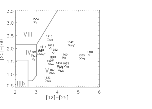
Figure 1: IRAS color-color diagram. The squares represent objects having Br$\gamma$ in absorption, the asterisks objects having Br$\gamma$ in emission and the crosses flat spectrum sources. Diamonds indicate sources for which the near-infrared counterpart is not certain. The objects are labeled by the first four numbers of their IRAS name. The SED class of each object is indicated next to its symbol. The boxes as defined by van der Veen & Habing (vdVeen88 (1988)) are drawn in.

In Fig. 1 we show the IRAS color-color diagram. The IRAS fluxes were converted to magnitudes according to the IRAS Explanatory Supplement (Beichman et al. Beichman84 (1984)). The boxes defined by van der Veen & Habing (vdVeen88 (1988)) are drawn in. According to this classification scheme, PNe are found in region V of the color-color diagram and AGB stars in region IV. In region VIII there may be some confusion from galaxies and young stellar objects, and in region IV an odd H ii region may be present. The only object in region VIII is IRAS 15544$-$5332, which is not redshifted and shows Br$\gamma$ in emission. The object is unresolved, and the Br$\gamma$ emission is very weak. Hence it is unlikely to be an ultra-compact H ii region, but we cannot completely rule out that it is an embedded young stellar object that is not hot enough to ionize its surroundings. IRAS 13416$-$6243 in region IV has Br$\gamma$ in absorption and hence can be considered to be a post-AGB star. ¿From the results in Fig. 1, it seems that in the IRAS color-color diagram no distinction can be made between post-AGB stars with Br$\gamma$ in emission, absorption, or a flat Br$\gamma$ spectrum. Post-AGB stars were expected to be located in a region in the IRAS color-color diagram between AGB stars and PNe (e.g. Volk & Kwok Volk89 (1989); van der Veen et al. vdVeen89 (1989); Hu et al. Hu93 (1993)). However van Hoof et al. (vHoof97 (1997)) found in their parameter study of the spectral evolution of post-AGB stars that they can follow a variety of paths in the IRAS color-color diagram. Consequently PNe and post-AGB stars can occupy the same region in the IRAS color-color diagram and the position in the IRAS color-color diagram alone cannot a priori give a unique determination of the evolutionary status of a post-AGB star. Our observations confirm this result.

The fact that our objects are mostly selected from the region where PNe were found and not in the region between AGB and PNe, may explain our high detection rate of Br$\gamma$ emission (for comparison, the search by Käufl et al. (Kaufl93 (1993)) for Br$\alpha$ emission in a sample of 21 post-AGB stars resulted in only one detection).

5.5.2 Near-infrared color-color diagrams

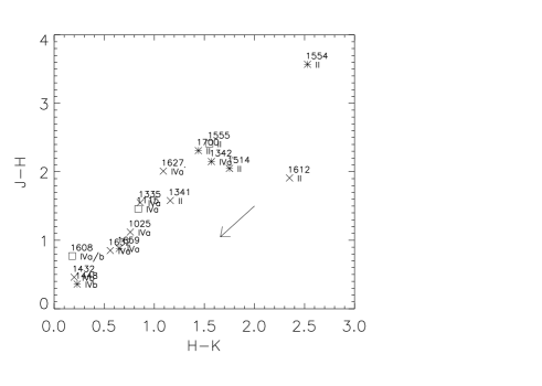
Figure 2: J$-$H versus H$-$K diagram. The symbols are defined in Fig. 1. The arrow shows the effect of correcting for $A_{V}$ = 5 mag.

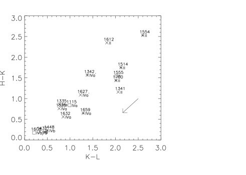
Figure 3: H$-$K versus K$-$L diagram. The symbols are defined in Figs. 1 and 2.

In Fig. 2 and Fig. 3 we show the J$-$H versus H$-$K and the H$-$K versus K$-$L color-color diagrams, respectively. In the diagrams we notice that objects of class II are redder than the objects of class IV. The former are found in the top right part of the diagrams while the latter are located more towards the bottom left. The separation is most obvious in Fig. 3. For our sample, objects having K$-$L $>$ 1.5 mag are all of class II and objects which have a maximum in the near-infrared beyond 2 $\mu$m have H$-$K $>$ 1.0 mag. Objects for which the stellar signature is more pronounced and which peak more towards shorter wavelengths in the near-infrared, are found more towards the bottom left in the diagrams.

To understand this effect, we would like to point out that for all but the coolest stars the intrinsic shape of the stellar continuum in the near-infrared can be approximated by a Rayleigh-Jeans tail. Since the shape of this tail does not depend on stellar temperature, the intrinsic infrared colors of these stars will not depend on stellar temperature either. Furthermore, since the colors of an A0V star are by definition zero, the infrared colors for most other stars are also close to zero, except when severe inter- or circum-stellar extinction is present. In this case the infrared colors will be positive and can be used as a crude measure for the extinction.

The mass loss rate during the superwind phase is very high. At the end of this phase the circumstellar dust will almost completely obscure the central star. During the post-AGB evolution, as the AGB shell expands, the shell will become more optically thin to stellar radiation. The stellar signature becomes more pronounced and will peak towards ever shorter wavelengths in the near-infrared. Consequently, it is expected that post-AGB stars will move from the upper right of the diagram to the lower left as the AGB shell expands and the circumstellar extinction becomes less. Generally speaking, we might expect that the objects in the top right of the diagram have left the AGB more recently than the objects in the lower left. However, we need to be cautious about such an interpretation because of the combined effects of many unknowns. The time it takes for the envelope to become optically thin will depend upon the mass loss rate at the tip of the AGB, the wind velocity, and the distribution of the mass in the circumstellar shell. If the AGB star had a non-spherical mass loss concentrated towards the equator, the central star could be visible along polar directions, while being completely obscured in equatorial directions. Hence, the observed amount of circumstellar extinction will depend on the viewing angle (Soker Soker99 (1999)). The interstellar extinction also affects the position of the objects in the color-color diagrams, as indicated by the arrow. The J$-$H versus H$-$K diagram is clearly the most affected by interstellar extinction. Eleven of the 16 objects are within one degree of the galactic plane, including the 6 objects in class II. The two objects in class IVb also have the highest latitude ($|b|>$ $4^{\circ}$). We calculated the extinction for our objects at a distance of 1 kpc and 4 kpc according to Hakkila et al. (Hakkila97 (1997)): $A_{V}$ would be between 0.5 mag and 2.0 mag if the objects were at a distance of 1 kpc and between 2.1 mag and 6.2 mag with a median of 4.6 mag if they were at 4 kpc.

Objects with Br$\gamma$ in emission, absorption, or a flat spectrum are well mixed in the diagrams. As discussed in the previous section it is unlikely that the stars with Br$\gamma$ in emission have reached a temperature high enough to start to ionize the AGB shell and the emission probably originates in the stellar wind. Because we observe Br$\gamma$ in emission from objects in class II (e.g. IRAS 15144$-$5812), it seems that a fast stellar wind can be present at an early stage when the circumstellar shell is still very optically thick. We are currently trying to determine spectral types of our objects in order to determine their true post-AGB evolutionary status (Van de Steene et al., in preparation).

5.5.3 Combined near- and far-infrared color-color diagrams

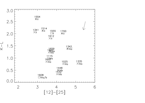
Figure 4: K$-$L versus [12]$-$[25] diagram. The symbols are defined in Figs. 1 and 2.

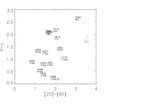
Figure 5: K$-$L versus [25]$-$[60] diagram. The symbols are defined in Figs. 1 and 2.

In Fig. 4 and Fig. 5 we show the K$-$L versus [12]$-$[25] and K$-$L versus [25]$-$[60] diagrams, respectively. The K$-$L color roughly describes the evolution of the circumstellar extinction and is therefore a measure for the expansion of the AGB shell, while the [12]$-$[25] and [25]$-$[60] colors reflect the evolution of the spectrum of the circumstellar dust shell.

In Fig. 4 we see a weak trend towards cooler [12]$-$[25] colors with decreasing K$-$L color at first. When K$-$L $<$ 1.5 mag this trend seems to reverse, probably due to an increase in 12 $\mu$m flux. However, this trend will need to be confirmed with a larger sample.

In Fig. 5 we see a broad and weak trend towards hotter [25]$-$[60] colors with decreasing K$-$L color. Obviously the 25-$\mu$m flux increases faster than the 60-$\mu$m flux.

Theoretical calculations by Blöcker (Bloecker95 (1995)) predict that directly after the star leaves the AGB, the stellar evolution is slow. This causes the AGB dust shell to cool when it expands. However, around $T_{\rm eff}\approx 8000$ K the evolution of the central star speeds up considerably and the grains in the AGB shell start to heat up again. This effect is most pronounced for silicate grains because, as the peak of the stellar spectrum moves into the UV, the efficiency with which these grains absorb light increases significantly. This causes the counter-clockwise loop which was first predicted by van Hoof et al. (vHoof97 (1997)) for oxygen-rich post-AGB stars in the IRAS color-color diagram. This effect could explain the reverse trend in Fig. 4, and also the trend in Fig. 5.

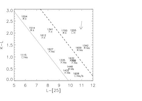
Figure 6: K$-$L versus L$-$[25] color-color diagram. The symbols are defined in Figs. 1 and 2. The dotted and dashed lines are explained in the text.

In Fig. 6 we plot the K$-$L versus L$-$[25] diagram. The K$-$L color describes the evolution of the circumstellar extinction. The L$-$[25] color relates the stellar component with the peak of the dust emission.

Because he K$-$L color is sensitive to the extinction and the L$-$[25] color is insensitive to extinction, all class II objects are found in the upper half of the diagram and class IV objects in the lower half.

For our limited sample, all but one of the objects are found to the right of the dotted line. This is partly due to sample selection. As the arrow indicates, objects less obscured (e.g., due to orientation along the polar axis, or because of an optically thin shell, or less interstellar extinction), and especially the ones with cool central stars, could be situated below the dotted line.

IRAS 11159$-$5954 has a lower extinction than its L$-$[25] color would indicate. This is an M-type star (Van de Steene et al., 2000, in preparation), which may still have ongoing mass loss. Its dust shell does not appear to be very thick and the star is very bright in the near infrared.

The objects to the right of the dashed line are extended in the near-infrared or the optical. IRAS 17009$-$4154 and IRAS 15553$-$5230 showed elliptical morphology. The former is very faint in the optical, the latter invisible. IRAS 13428$-$6232 shows a bipolar morphology in the near-infrared and and is also very faint in the optical. IRAS 16594$-$4656 is bright and was not observed to be extended in the near-infrared, though it showed a bipolar morphology in its HST image (Hrivnak et al. Hrivnak99 (1999)). Probably they have a thicker cool circumstellar dust shell than objects located below the dashed line (more 25 $\mu$m-band flux) and/or their central star temperatures are higher (less L-band flux).

As the dust shell expands, the [25] magnitude will decrease a bit (for oxygen-rich post-AGB stars) or remain roughly constant (for carbon-rich post-AGB stars) (van Hoof et al. vHoof97 (1997)). The L magnitude will increase, as the stellar temperature increases. The K magnitude will decrease as the star starts shining through the dust shell. Thus the L$-$[25] values are expected to increase with decreasing K$-$L values as the shell expands and the star becomes hotter.

This is what we observe in Fig. 6, both for the extended and non-extended objects. A small L$-$[25] color indicates that the system is young, hence the star is heavily obscured by the dust shell which is still close to the star. This is noticeable by the large K$-$L values. For objects with a larger L$-$[25] color the AGB shell is already more detached and cooler. The extinction is less and this translates into a smaller value for the K$-$L color.

The K$-$L versus L$-$[12] diagram (not shown) is very similar to the K$-$L versus L$-$[25] diagram, but the spread is larger for K$-$L $<$ 1.0 mag, possibly because of an increase in 12-$\mu$m flux, as discussed in the previous section. Because of its relatively large 12-$\mu$m flux, IRAS 13416$-$6342 is located close to IRAS 17009$-$4154. It needs to be checked at higher resolution whether this source is extended.

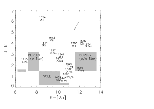
Figure 7: J$-$K versus K$-$[25] color-color diagram. The symbols are defined in Figs. 1 and 2. The grey regions show the location of objects in Ueta et al.(Ueta00 (2000)). These regions are labeled according to their definitions as SOLE and DUPLEX with and without star. The dashed line separates the two kind of objects.

In Fig. 7 we show the color-color diagram proposed by Ueta et al. (Ueta00 (2000)). Since the J$-$K color measures the circumstellar extinction, in a similar way as K$-$L color does, and because the evolution described above for the L$-$[25] color is equally valid for the K$-$[25] color, one would expect the same decreasing trend as in the previous diagram. However, extinction effects have a much stronger effect on the K$-$[25] and J$-$K colors than on the L$-$[25] and K$-$L colors, as can be seen from the arrows in both diagrams. Nearly all objects of class IVa have J$-$K $<$ 2.5 mag. When the star becomes prominent in the near-infrared, the stellar maximum shifts through the K-band towards the J-band, causing a reversal in the evolutionary trend.
The extended objects are also found towards the right of the diagram. In this plot it is more obvious that IRAS 16594$-$4656 is the brightest of the 4 extended objects.

Ueta et al. (Ueta00 (2000)) had one M star, IRAS 04386$+$5722, offset towards blue K$-$[25] color, similar to IRAS 11159$-$5954, but a bit bluer in J$-$K. Its position is indicated with the smallest grey box in Fig. 7.

The long-dashed line at J$-$K = 1.45 mag in Fig. 7 separates the regions what Ueta et al. call Star-Obvious Low level Elongated (SOLE) and DUst Prominent Longitudinally EXtended (DUPLEX) nebulae. One quarter of our objects would be classified as SOLE and three quarters as DUPLEX in this scheme. The grey regions show where the objects in their sample are located and are labeled with their acronyms. Our samples are obviously complementary: there is virtually no overlap ! The difference may be caused in part by the selection criteria. They have selected known post-AGB candidates from the literature and imaged their nebulosities with WFPC2 in the optical. Consequently they chose optically bright post-AGB stars. We selected objects from the PNe region in the IRAS color-color diagram of which very few had an optical counterpart identified. Moreover, all our objects are located within 5 degrees of the galactic plane, while only 11 out of their 27 objects are (3 SOLE, 6 DUPLEX, and 2 stellar). The arrow in the diagram indicates a correction for $A_{V}$ = 5 mag of extinction. Larger interstellar extinction alone cannot explain why our samples appear different. If the objects in both samples are at similar distances, it is plausible that we have more massive central stars in our sample, and that they are evolving faster across the HR diagram. Further investigation is needed to understand the differences between both samples.

In summary, no distinction can be made between the objects showing Br$\gamma$ in emission, absorption, or a flat spectrum, in any of the color-color diagrams. The trends we see in the near and far infrared are mainly due to the expansion, morphology, and dust properties in the circumstellar shell and the obscuration of the central star it causes. The trends show the expected evolution of the circumstellar shell. Whether the positions of the objects in the color-color diagrams can be directly related to the temperature and core mass of the central star needs further investigation.

6 Conclusions

In this article we reported further investigations of the IRAS selected sample of PN candidates that was presented in Van de Steene & Pottasch (VdSteene93 (1993)). About 20 % of the candidates in that sample have been detected in the radio and/or H$\alpha$ and were later confirmed as PNe. Here we investigated the nature of the non-radio-detected sources.

• Of sixteen positively identified objects, seven show Br$\gamma$ in absorption. The absorption lines are very narrow in six objects, indicating a low surface gravity. This is a strong indication for the post-AGB nature of these objects. Another six objects show Br$\gamma$ in emission. Two of these also show photospheric absorption lines. All emission line sources have a strong underlying continuum, unlike normal PNe. In another three objects, no clear Br$\gamma$ absorption or emission was visible.

• The objects showing Br$\gamma$ in emission were re-observed in the radio continuum with the Australia Telescope Compact Array. None of them were detected above a detection limit of 0.55 mJy/beam at 6 cm and 0.7 mJy/beam at 3 cm, while they should have been easily seen if the radio emission was optically thin and Case B recombination was applicable. It is argued that the Br$\gamma$ emission may be due to ionization in the post-AGB wind, present before the star is hot enough to ionize the AGB shell.

• The fact that our objects were mostly selected from the region in the IRAS color-color diagram where typically PNe are found, may explain our higher detection rate of emission line objects compared to previous studies, which selected their candidates from a region between AGB and PNe. These post-AGB stars also cover a larger range in color and are generally much redder than the ones known so far.

• In the near-infrared color-color diagrams our objects cover a very large range of extinction. Near-infrared versus far-infrared color-color diagrams show trends which reflect the expected evolution of the expanding circumstellar shell. No distinction can be made between the objects showing Br$\gamma$ in emission, absorption, or a flat spectrum in the near- and far-infrared color-color diagrams. Whether the positions of the objects in the color-color diagrams can be directly related to the temperature and core mass of the central star needs further investigation.

• We identified the K$-$L versus L$-$[25] diagram as a potentially useful tool to distinguish: 1) extended from unresolved post-AGB stars, and 2) obscured objects of class II having thick circumstellar shells from the brighter class IV objects which show a stellar signature in their near-infrared SEDs. However, this result should be confirmed with a larger sample.

Figure 8: Countour plots of resolved objects in the N-band. The positions not corrected for the pointing errors of the ESO 3.6-m telescope.

Figure 9: The caspir K-band images of the IRAS sources. The IRAS position is indicated with a cross and the object observed with irspec is in the box. The encircled object might be a more likely IRAS counterpart. The pixelsize is 0$\aas@@fstack{\prime\prime}$25 and the FOV 1′$\times$ 1′. North is up and East to the left.

These images are supplied as 20 separate jpeg images (im1025K.jpg through im1708K.jpg).

Figure 10: We present the spectral energy distribution of the sources: plotted are the near-infrared JHKL flux values at 1.29 $\mu$m, 1.65 $\mu$m, 2.20 $\mu$m, and 3.85 $\mu$m respectively, and the far-infrared IRAS 12-$\mu$m, 25-$\mu$m, and 60-$\mu$m flux values.

Figure 11: The normalized spectra of the objects with Br$\gamma$ in emission, absorption, and objects for which no Br$\gamma$ was detected in absorption or emission.

- (1) Beichman C.A., Neugebauer G., Habing H.J., Clegg P.E., Chester T.J., 1984, IRAS Catalogs and Atlases Explanatory Supplement
- (2) Blöcker T., 1995, A&A 299, 755
- (3) Epchtein N., de Batz B., Copet E., et al., 1994, Ap&SS 217, 3
- (4) Frank A., Balick B., Icke V., Mellema G., 1993, ApJ 404, L25
- (5) García-Lario P., Manchado A., Pych W., Pottasch S.R., 1997, A&A 126, 479
- (6) Hakkila J., Myers J.M., Stidham B.J., Hartmann D.H., 1997, AJ 114, 2043
- (7) Hirshfeld A., Sinnott R.W., Ochsenbein F., 1991, Sky Catalogue 2000.0 2nd ed., Sky Publishing Corporation, Cambridge Massachusetts
- (8) Hrivnak B.J., Kwok S., Su K.Y.L., 1999, ApJ 524, 849
- (9) Hu J.Y., Slijkhuis S., de Jong T., Jiang B.W., 1993, A&AS 100, 413
- (10) Käufl H.U., Renzini A., Stanghellini L., 1993, ApJ 410, 251
- (11) Knapp G.R., Bowers P.F., Young K., Philips T.G., 1995, ApJ 455, 293
- (12) Kwok S., 1982, ApJ 258, 280
- (13) McGregor P., 1994, caspir manual, http://www.mso.anu.edu.au/observing/teldocs/2.3m/CASPIR
- (14) Oliva E., Origlia L., 1992, A&A 254, 466
- (15) Sahai R., Trauger J.T., 1998, AJ 113, 1357
- (16) Soker N., 1999, MNRAS, submitted (astro-ph/9912015)
- (17) Solf J., 1994, A&A 282, 567
- (18) Ueta T., Meixner M., Bobrowsky M., 2000, ApJ 528, 861
- (19) van der Veen W.E.J.C., Habing H.J., 1988, A&A 194, 125
- (20) van der Veen W.E.J.C., Habing H.J., Geballe T.R., 1989, A&A 226, 108
- (21) Van de Steene G.C., Pottasch S.R., 1993, A&A 274, 895
- (22) Van de Steene G.C., Pottasch S.R., 1995, A&A 299, 238
- (23) Van de Steene G.C., Jacoby G.H., Pottasch S.R., 1996, A&AS 118, 243
- (24) Van de Steene G.C., Sahu K.S., Pottasch S.R., 1996, A&AS 120, 111
- (25) Van de Steene G.C., Wood P.R., van Hoof P.A.M., 2000, in Kastner J.H., Soker N., Rappaport S.A. (eds.) Asymmetrical Planetary Nebulae II: from Origins to Microstructures. ASP Conference Series, Vol. 199, p. 191
- (26) van Hoof P.A.M., Oudmaijer R.D., Waters L.B.F.M., 1997, MNRAS 289, 371
- (27) Volk K.M., Kwok S., 1989, ApJ 342, 345