Genetic-Algorithm-based Asteroseismological Analysis
of the DBV White Dwarf GD 358

Abstract

White dwarf asteroseismology offers the opportunity to probe the structure and composition of stellar objects governed by relatively simple physical principles. The observational requirements of asteroseismology have been addressed by the development of the Whole Earth Telescope (WET), but the analytical procedures still need to be refined before this technique can yield the complete physical insight that the data can provide. Toward this end, we have utilized a genetic-algorithm-based optimization method to fit our models to the observed pulsation frequencies of the DBV white dwarf GD 358 obtained with the WET in 1990. This new approach has finally exploited the sensitivity of our models to the core composition, and will soon yield some interesting constraints on nuclear reaction cross-sections.

Accepted for publication in the Astrophysical Journal

1 INTRODUCTION

We study white dwarf stars because they are the end-points of stellar evolution for the majority of all stars, and their composition and structure can tell us about their prior history. We can determine the internal structure of pulsating white dwarfs by observing their variations in brightness over time, using the techniques of high speed photometry to define their light curves, and then matching these observations with a numerical model which behaves the same way. The parameters of the model are chosen to correspond one-to-one with the physical processes that give rise to the variations, so a good fit to the data leads us to believe that our model reflects the actual physics of the stars themselves.

Although this procedure is simple in outline, its realization in practice requires specialized instrumentation to overcome the practical difficulties we encounter in the process. The Whole Earth Telescope (WET) observing network (Nather et al., 1990) was developed to provide the 200 or more hours of essentially gap-free data we require for the analysis. This instrument is now mature, and has provided a wealth of seismological data on the different varieties of pulsating white dwarf stars, so the observational part of the procedure is well in hand. Now we are working to improve our analytical procedures to take full advantage of the possibilities afforded by asteroseismology.

The adjustable parameters in our computer models of white dwarfs presently include the total mass, the temperature, hydrogen and helium layer masses, core composition, convective efficiency, and composition transition profiles. Finding a proper set of these to provide a close fit to the observed data is difficult. The traditional procedure is a cut-and-try process guided by intuition and experience, and is far more subjective than we would like. More objective procedures are essential if asteroseismology is to become a widely-accepted astronomical technique. We must be able to demonstrate that, within the range of different values the model parameters can assume, we have found the only solution or the best one if more than one is possible.

2 GENETIC ALGORITHMS

An optimization scheme based on a genetic algorithm (GA) can avoid the problems inherent in the traditional approach. Restrictions on the range of the parameter-space are imposed only by observational constraints and by the physics of the model. Although the parameter-space so defined is often quite large, the GA provides a relatively efficient means of searching globally for the best-fit model. While it is difficult for GAs to find precise values for the best-fit set of parameters, they are very good at finding the region of parameter-space that contains the global minimum. In this sense, the GA is an objective means of finding a good first guess for a more traditional method which can then narrow in on the precise values and uncertainties of the best-fit set of parameters.

The underlying ideas for genetic algorithms were inspired by Charles Darwin’s (1859) notion of biological evolution through natural selection. The basic idea is to solve an optimization problem by evolving the best solution from an initial set of completely random guesses. The theoretical model provides the framework within which the evolution takes place, and the individual parameters controlling it serve as the genetic building blocks. Observations provide the selection pressure. For a detailed description of genetic algorithms, see Metcalfe (1999) and Charbonneau (1995).

Initially, the parameter-space is filled uniformly with trials consisting of randomly chosen values for each parameter, within a range based on the physics that the parameter is supposed to describe. The model is evaluated for each trial, and the result is compared to the observed data and assigned a fitness inversely proportional to the variance. A new generation of trials is then created by selecting from this population at random, weighted by the fitness.

Each model is encoded into a long string of numbers analogous to a chromosome with each parameter serving as a gene. The encoded trials are paired up and modified in order to explore new regions of parameter-space. The two basic genetic operators are crossover which emulates reproduction, and mutation which emulates happenstance. After these operators have been applied, the strings are decoded back into sets of numerical values for the parameters. The new generation replaces the old one, and the process begins again. The evolution continues for a specified number of generations, chosen to maximize the efficiency of the method.

3 THE DBV WHITE DWARF GD 358

During a survey of eighty-six suspected white dwarf stars in the Lowell GD lists, Greenstein (1969) classified GD 358 as a helium atmosphere (DB) white dwarf based on its spectrum. Photometric $UBV$ and $ubvy$ colors were later determined by Bern & Wramdemark (1973) and Wegner (1979) respectively. Time-series photometry by Winget Robinson Nather & Fontaine (1982) revealed the star to be a pulsating variable—the first confirmation of a new class of variable (DBV) white dwarfs predicted by Winget (1981).

In May 1990, GD 358 was the target of a coordinated observing run with the WET. The results of these observations were reported by Winget et al. (1994), and the theoretical interpretation was given in a companion paper by Bradley & Winget (1994b). They found a series of nearly equally-spaced periods in the power spectrum which they interpreted as non-radial g-mode pulsations of consecutive radial overtone. They attempted to match the observed periods and the period spacing for these modes using earlier versions of the same theoretical models we have used in this analysis (see §LABEL:MODSECT). Their optimization method involved computing a grid of models near a first guess determined from general scaling arguments and analytical relations developed by Kawaler (1990), Kawaler & Weiss (1990), Brassard Fontaine Wesemael & Hansen (1992), and Bradley Winget & Wood (1993).

4 DBV WHITE DWARF MODELS

4.1 Defining the Parameter-Space

The most important parameters affecting the pulsation properties of DBV white dwarf models are the total stellar mass ($M_{*}$), the effective temperature ($T_{\rm eff}$), and the mass of the atmospheric helium layer ($M_{\rm He}$). We want to be careful to avoid introducing any subjective bias into the best-fit determination simply by defining the range of the search too narrowly. For this reason, we have specified the range for each parameter based only on the physics of the model, and on observational constraints.

The distribution of masses for isolated white dwarf stars, generally inferred from measurements of $\log\ g$, is strongly peaked near 0.6 $M_{\odot}$ with a FWHM of about 0.1 $M_{\odot}$ (Napiwotzki Green & Saffer, 1999). Isolated main sequence stars with masses near the limit for helium ignition produce C/O cores more massive than about 0.45 $M_{\odot}$, so white dwarfs with masses below this limit must have helium cores (Sweigart Greggio & Renzini, 1990; Napiwotzki Green & Saffer, 1999). However, the universe is not presently old enough to produce helium core white dwarfs through single star evolution. We confine our search to masses between 0.45 $M_{\odot}$ and 0.95 $M_{\odot}$. Although some white dwarfs

3.5in gd358.fig1.ps

The numerical thin limit of the fractional helium layer mass for various values of the total mass (connected points) and the linear cut implemented in the WD-40 code (dashed line).

are known to be more massive than the upper limit of our search, these represent a very small fraction of the total population, and for reasonable assumptions about the mass-radius relation all known DBVs appear to have masses within the range of our search (Beauchamp et al., 1999).

The span of effective temperatures within which DB white dwarfs are pulsationally unstable is known as the DB instability strip. The precise location of this strip is the subject of some debate, primarily because of difficulties in matching the temperature scales from ultraviolet and optical spectroscopy and the possibility of hiding trace amounts of hydrogen in the envelope (Beauchamp et al., 1999). The most recent temperature determinations for the 8 known DBV stars were done by Beauchamp et al. (1999). These measurements, depending on various assumptions, place the red edge as low as 21,800 K, and the blue edge as high as 27,800 K. Our search includes all temperatures between 20,000 K and 30,000 K.

The mass of the atmospheric helium layer must not be greater than about $10^{-2}\ M_{*}$ or the pressure of the overlying material would theoretically initiate helium burning at the base of the envelope. At the other extreme, none of our models pulsate for helium layer masses less than about $10^{-8}\ M_{*}$ over the entire temperature range we are considering (Bradley & Winget, 1994a). The practical limit is actually slightly larger than this theoretical limit, and is a function of mass. For the most massive white dwarfs we consider, our models run smoothly with a helium layer as thin as $5\times 10^{-8}\ M_{*}$, while for the least massive the limit is $4\times 10^{-7}\ M_{*}$ (see Figure 1).

4.2 Theoretical Models

To find the theoretical pulsation modes of a white dwarf, we start with a static model of a pre-white dwarf and allow it to evolve quasi-statically until it reaches the desired temperature. We then calculate the adiabatic non-radial oscillation frequencies for the output model. The initial ‘starter’ models can come from detailed calculations that evolve a main-sequence star all the way to its pre-white dwarf phase, but this is generally only important for accurate models of the hot DO white dwarfs. For the cooler DB and DA white dwarfs, it is sufficient to start with a hot polytrope of order 2/3 (i.e. $P\propto\rho^{5/3}$). The cooling tracks of these polytropes converge with those of the pre-white dwarf models well above the temperatures at which DB and DA white dwarfs are observed to be pulsationally unstable (Wood, 1990).

To allow fitting for the total mass, we generated a grid of 100 starter models with masses between 0.45 and 0.95 $M_{\odot}$. The entire grid originated from a 0.6 $M_{\odot}$ carbon-core polytrope starter model. We performed a homology transform on this model to generate three new masses: 0.65, 0.75, and 0.85 $M_{\odot}$. We relaxed each of these three, and then used all four to generate the grid. All models with masses below 0.6 $M_{\odot}$ were generated by a direct homology transform of the original 0.6 $M_{\odot}$ polytrope. For masses between $0.605\rightarrow 0.745$ $M_{\odot}$ and from $0.755\rightarrow 0.895$ $M_{\odot}$, we used homology transforms of the relaxed 0.65 $M_{\odot}$ and 0.75 $M_{\odot}$ models respectively. The models with masses greater than 0.9 $M_{\odot}$ were homology transforms of the relaxed 0.85 $M_{\odot}$ model.

To evolve a starter model to a specific temperature, we used the White Dwarf Evolution Code (WDEC) described in detail by Lamb & van Horn (1975) and by Wood (1990). This code was originally written by Martin Schwarzschild, and has subsequently been updated and modified by many others including: Kutter & Savedoff (1969), Lamb & van Horn (1975), Winget (1981), Kawaler (1986), Wood (1990), Bradley (1993), and Montgomery (1998). The equation of state (EOS) for the cores of our models come from Lamb (1974), and from Fontaine Graboske & Van Horn (1977) for the envelopes. We use the updated OPAL opacity tables from Iglesias & Rogers (1993), neutrino rates from Itoh et al. (1989), and the ML3 mixing-length prescription of Böhm & Cassinelli (1971). The evolution calculations for the core are fully self-consistent, but the envelope is treated separately. The core and envelope are stitched together and the envelope is adjusted to match the boundary conditions at the interface. Adjusting the helium layer mass involves stitching an envelope with the desired thickness onto the core before starting the evolution. Because this is done while the model is still very hot, there is plenty of time to reach equilibrium before the model approaches the final temperature.

We determined the pulsation frequencies of the output models using the adiabatic non-radial oscillation (ANRO) code described by Kawaler (1986), originally written by Carl Hansen, which solves the pulsation equations using the Runge-Kutta-Fehlberg method.

We have made extensive practical modifications to these programs, primarily to allow models to be calculated without any intervention by the user. The result is a combined evolution/pulsation code that runs smoothly over a wide range of input parameters. We call this new code WD-40. Given a mass, temperature, and helium layer mass within the ranges discussed above, WD-40 will evolve and pulsate the specified white dwarf model and return a list of the theoretical pulsation periods.

5 MODEL FITTING

The execution time for a single DB model on a reasonably fast computer is less than a minute. The genetic algorithm approach, however, requires the evaluation of many thousands of such models. To be practical, we ran the code in parallel on a specialized computational instrument—a collection of minimal PCs connected by a network—which we designed and built for this project (see Metcalfe & Nather, 1999a, b).

We used the most recent version of a public-domain GA (called PIKAIA) described in detail by Charbonneau (1995). To allow the evaluation of models in parallel, we incorporated the message passing routines of the Parallel Virtual Machine (PVM) software (Geist et al., 1994) into the “full generational replacement” evolution option of PIKAIA.

Our strategy was to use PIKAIA as a master program to exchange data with many copies of the WD-40 code serving as slave processes. The master program sends sets of parameters to slave processes running on every available processor, and then listens for responses. It sends new jobs after each response, and continues until all of the trials for a particular generation have been calculated. The master program then performs the genetic shuffling to come up with a new generation of trials to be calculated. This continues for a specified number of generations, and the best solution in the final population of trials is used as the first guess for a more traditional approach.

The slave processes, when they receive data from the master program, evolve a white dwarf model with the specified properties, calculate the pulsation periods, and compare them to the observed periods. The relative fitness of the trial—which we define as the inverse of the root-mean-square (r.m.s.) residuals between the observed and calculated pulsation periods—is then sent back to the master program.

We used a population size of 128 trials, and initially allowed the GA to run for 250 generations. We used 2-digit decimal encoding for each of the three parameters, which resulted in a temperature resolution of 100 K, a mass resolution of 0.005 $M_{\odot}$, and a resolution for the helium layer thickness of 0.05 dex. The uniform single-point crossover probability was fixed at 85%, and the mutation rate was allowed to vary between 0.1% and 16.6%, depending on the linear distance in parameter-space between the trials with the median and the best fitnesses.

5.1 Application to Noiseless Simulated Data

To quantify the efficiency of our method for this problem, we used the WD-40 code to calculate the pulsation periods of a model within the search space, and then attempted to find the set of input parameters [$T_{\rm eff}=25,000$ K, $M_{*}=0.600$ $M_{\odot}$, $\log(M_{\rm He}/M_{*})=-5.96$] using the GA. We performed 20 independent runs using different pseudo-random number sequences each time. The first order solutions found in each case by the GA are listed in Table 1. In 9 of the 20 runs, the GA found the exact set of input parameters, and in 4 other runs it finished in a region of parameter-space close enough for a small (1331 point) grid to reveal the exact answer. Since none

Table 1

Results for Noiseless Simulated Data

	First-Order Solution				Generation
Run	$T_{\rm eff}$	$M/M_{\odot}$	$\log(M_{\rm He}/M_{*})$	r.m.s.	Found
01	26,800	0.560	$-$5.70	0.67	245
02	25,000	0.600	$-$5.96	0.00	159
03	24,800	0.605	$-$5.96	0.52	145
04	25,000	0.600	$-$5.96	0.00	68
05	22,500	0.660	$-$6.33	1.11	97
06	25,000	0.600	$-$5.96	0.00	142
07	25,000	0.600	$-$5.96	0.00	97
08	25,000	0.600	$-$5.96	0.00	194
09	25,200	0.595	$-$5.91	0.42	116
10	26,100	0.575	$-$5.80	0.54	87
11	23,900	0.625	$-$6.12	0.79	79
12	25,000	0.600	$-$5.96	0.00	165
13	26,100	0.575	$-$5.80	0.54	92
14	25,000	0.600	$-$5.96	0.00	95
15	24,800	0.605	$-$5.96	0.52	42
16	26,600	0.565	$-$5.70	0.72	246
17	24,800	0.605	$-$5.96	0.52	180
18	25,000	0.600	$-$5.96	0.00	62
19	24,100	0.620	$-$6.07	0.76	228
20	25,000	0.600	$-$5.96	0.00	167

of the successful runs converged between generations 200 and 250, we stopped future runs after 200 generations.

From the 13 runs that converged in 200 generations, we deduce an efficiency for the method (GA + small grid) of $\sim$65%. This implies that the probability of missing the correct answer in a single run is $\sim$35%. By running the GA several times, we reduce the probability of not finding the correct answer: the probability that two runs will both be wrong is $\sim$12%, for three runs it is $\sim$4%, and so on. Thus, to reduce the probability of not finding the correct answer to below 1% we need to run the GA, on average, 5 times. For 200 generations of 128 trials, this requires $\sim$10⁵ model evaluations. By comparison, an exhaustive search of the parameter-space with the same resolution would require $10^{6}$ model evaluations, so our method is comparably global but $\sim$10$\times$ more efficient than an exhaustive search of parameter-space. Even with this efficiency and our ability to run the models in parallel, each run of the GA required about 6 hours to complete.

5.2 The Effect of Gaussian Noise

Having established that the GA could find the correct answer for noiseless data, we wanted to see how noise on the frequencies might affect it. Before adding noise to the input frequencies, we attempted to characterize the actual noise present on frequencies determined from a WET campaign. We approached this problem in two different ways.

First, we tried to characterize the noise empirically using the mode identifications from Vuille et al. (2000) to look at the distribution of differences between the observed and predicted linear combination frequencies in the 1994 WET run on GD 358. There were a total of 63 combinations identified: 20 sum and 11 difference frequencies of 2-mode combinations, 30 sum and difference 3-mode combinations, and 2 combinations involving 4 modes. We used the measured frequencies of the parent modes to predict the frequency of each linear combination, and then compared this to the observed frequency. The distribution of observed minus computed frequencies for these 63 modes, and the best-fit Gaussian is shown in the top panel of Figure 5.2. The distribution has $\sigma=0.17\ \mu$Hz.

Second, we tried to characterize the noise by performing the standard analysis for WET runs on many simulated light curves to look at the distribution of differences between the input and output frequencies. We generated 100 synthetic GD 358 light curves using the 57 observed frequencies and amplitudes from Winget et al. (1994). Each light curve had the same time span as the 1990 WET run (965,060 seconds) sampled with the same interval (every 10 seconds) but without any gaps in coverage. Although the noise in the observed light curves was clearly time-correlated, we found that the distribution around the mean light level for the comparison star after the standard reduction procedure was well represented by a Gaussian. So we added Gaussian noise to the simulated light curves to yield a signal-to-noise ratio $S/N\approx 2$, which is typical of the observed data. We took the discrete Fourier Transform of each light curve, and identified peaks in the same way as is done for real WET runs. We calculated the differences between the input frequencies and those determined from the simulation for the 11 modes used in the seismological analysis by Bradley & Winget (1994b). The distribution of these differences is shown in the bottom panel of Figure 5.2, along with the best-fit Gaussian which has $\sigma=0.053\ \mu$Hz. We adopted this value for our studies of the effects of noise on the GA method.

Using the same input model as in §5.1, we added random offsets drawn from a Gaussian distribution with $\sigma=0.053\ \mu$Hz to each of the frequencies. We produced 10 sets

3.5in gd358.fig2.ps

The distribution of differences between (a) the observed and predicted frequencies of linear combination modes identified by Vuille et al. (2000) in the 1994 WET run on GD 358 and the best-fit Gaussian with $\sigma=0.17\ \mu$Hz (dashed line) and (b) the input and output frequencies of the 11 modes used to model GD 358 from simulated WET runs (see §5.2 for details) and the best-fit Gaussian with $\sigma=0.053\ \mu$Hz (dashed line).

of target frequencies from 10 unique realizations of the noise, and then applied the GA method to each set. In all cases the best of 5 runs of the GA found the exact set of parameters from the original input model, or a region close enough to reveal the exact solution after calculating the small grid around the first guess. To reassure ourselves that the success of the GA did not depend strongly on the amount of noise added to the frequencies, we also applied the GA to several realizations of the larger noise estimate from the analysis of linear combination frequencies. The GA always succeeded in finding the original input model.

5.3 Application to GD 358

Having thoroughly characterized the GA method, we finally applied it to real data. We used the same 11 periods used by Bradley & Winget (1994b). As in their analysis, we assumed that the periods were consecutive radial overtones and that they were all $\ell=1$ modes. Anticipating that the GA might have more difficulty with non-synthetic data, we decided to perform a total of 10 GA runs for each core composition. This should reduce the chances of not finding the best answer to less than about 3 in 10,000.

To facilitate comparison with previous results, we obtained fits for six different combinations of core composition and transition profiles: pure C, pure O, and both “steep” and “shallow” transition profiles for 50:50 and 20:80 C/O cores (see Bradley Winget & Wood, 1993; Bradley & Winget, 1994b).

We also ran the GA with an alternate fitness criterion for the 50:50 C/O “steep” case, which contains the best-fit model of Bradley & Winget (1994b). Normally, the GA only attempts to match the pulsation periods. We reprogrammed it to match both the periods and deviations from the mean period spacing, which was the fitness criterion used by Bradley & Winget. Within the range of parameters they considered, using this alternate fitness criterion, the GA found best-fit model parameters consistent with Bradley & Winget’s solution.

6 RESULTS

The general features of the 3-dimensional parameter-space [$M_{*},T_{\rm eff},-\log_{10}(M_{\rm He}/M_{*})$] for GD 358 are illustrated in Figure 1. All combinations of parameters found by the GA for a 50:50 C/O steep core having r.m.s. period differences smaller than 3 seconds are shown as square points in this plot. The two panels are orthogonal projections of the search space, so each point in the left panel corresponds one-to-one with a point in the right panel. Essentially, Figure 1 shows which combinations of model parameters yield reasonably good matches to the periods observed in GD 358 for this core composition. The most obvious feature of the parameter-space is the presence of more than one region that yields a good match to the observations. Generally, the good fits seem to cluster in two groups corresponding to thick and thin helium layers. Also obvious are the parameter-degeneracies in both projections, causing the good fits to fall along a line in parameter-space rather than on a single point.

The parameter-degeneracy between total mass and fractional helium layer mass is relatively easy to understand. Brassard Fontaine Wesemael & Hansen (1992) showed that the pulsation periods of trapped modes in white dwarf models are strongly influenced by the scaled location of the composition transition zone. They developed an expression showing that these periods are directly proportional to the fractional radius of the composition interface. As the total mass of a white dwarf increases, the surface area decreases, so the mass of helium required to keep the interface at the same fractional radius also decreases. Thus, a thinner helium layer can compensate for an overestimate of the mass.

The parameter-degeneracy between mass and temperature is slightly more complicated. The natural frequency that dominates the determination of white dwarf model pulsation frequencies is the Brunt-Väisälä frequency (which reflects the difference between the actual and the adiabatic density gradients). As the temperature decreases, the matter becomes more degenerate, so the Brunt-Väisälä frequency in much of the star tends to zero. The pulsation periods of a white dwarf model in some sense reflect the average of the Brunt-Väisälä frequency throughout the star, so a decrease in temperature leads to lower pulsation frequencies. Higher mass models have higher densities, which generally lead to higher pulsation frequencies. So an overestimate of the mass can compensate for the effect of an underestimate of the temperature.

The results for all six core compositions and transition profiles are shown in Figure 2, where we have used color to indicate the absolute quality of each fit. We find that reasonable fits are possible with every core composition, but excellent fits (indicated by red points in the figure) are only possible for a specific core composition and transition profile. Pure C and pure O models appear to have more families of possible solutions, but the high-mass families have luminosities which are inconsistent with the observed parallax of GD 358 (Harrington et al., 1985). Mixed

7.0in gd358.fig3.ps

Figure 1: Front and side views of the GA search space for a C/O 50:50 core with a “steep” transition profile. Square points mark the locations of every model found by the GA with an r.m.s. deviation smaller than 3 seconds for the periods observed in GD 358. The dashed line shows the range of parameters considered by Bradley & Winget (1994b).

C/O cores generally seem to produce better fits, but transition profiles that are steep are much worse than those that are shallow. Among the mixed C/O cores with shallow transition profiles, the 20:80 mix produces the best fits of all.

The parameters for the best-fit models and measures of their absolute quality are listed in Table 7. For each core composition, the best-fit for both the thick and thin helium layer families are shown. As indicated, several fits can be ruled out based on their luminosities. Our new best-fit model for GD 358 has a mass and temperature marginally consistent with those inferred from spectroscopy.

7 DISCUSSION & FUTURE WORK

The genetic algorithm approach to asteroseismology has turned out to be very fruitful. We are now confident that we can rely on this new approach to perform global searches and to provide not only objective best-fit models for the pulsation frequencies of DBV white dwarfs, but also fairly detailed maps of the parameter-space as a natural byproduct. This approach can easily be extended to treat the DAV stars and, with a grid of more detailed starter models, eventually the DOVs. Ongoing all-sky surveys promise to yield many new pulsating white dwarfs of all classes which will require follow-up with the Whole Earth Telescope to obtain seismological data. With the observational and analytical procedures in place, we will quickly be able to understand the statistical properties of these ubiquitous and relatively simple objects.

This first application has confirmed that the pulsation frequencies of white dwarfs really are global oscillations. We have refined our knowledge of the sensitivity of our models to the structure of the envelope, and we have confirmed that they are sensitive to the conditions deep in the interior of the star, as was first demonstrated by the work on crystallization by Montgomery & Winget (1999).

The fact that our new best-fit solution has a thick helium layer may help to resolve a long-standing controversy surrounding the evolutionary connection between the PG 1159 stars and the DBVs. The helium layer mass for PG 1159-035 from the asteroseismological investigation of Winget et al. (1991) was $\sim 3\times 10^{-3}$ $M_{\odot}$ while the previous best-fit for GD 358 was $\sim 1.2\times 10^{-6}$ $M_{\odot}$. Dehner & Kawaler (1995) treated this problem by including time-dependent diffusive processes in their calculations, but admitted that the presence of the DB gap still remained a problem. The thick envelope solution could also allow GD 358 to fit comfortably within an evolutionary scenario leading to a carbon (DQ) white dwarf without developing an anomalously high photospheric carbon abundance.

Now that we have seen the significant improvement possible in the fits to GD 358 by searching globally for various core compositions, we can extend this method to treat the central C/O ratio as a free parameter. This has the exciting potential to place meaningful constraints on nuclear reaction cross-sections. During carbon burning, the triple-$\alpha$ process competes with the ${}^{12}{\rm C}(\alpha,\gamma)^{16}{\rm O}$ reaction for the available $\alpha$-particles. As a consequence, the final ratio of carbon to oxygen in the core is a measure of the relative cross-sections of these two reactions (Buchman, 1996). With more realistic transition profiles (e.g. Salaris et al., 1997) we hope to use GD 358 to measure this ratio, which is especially important for understanding type Ia supernovae.

We also plan to test the isotopic separation hypothesis

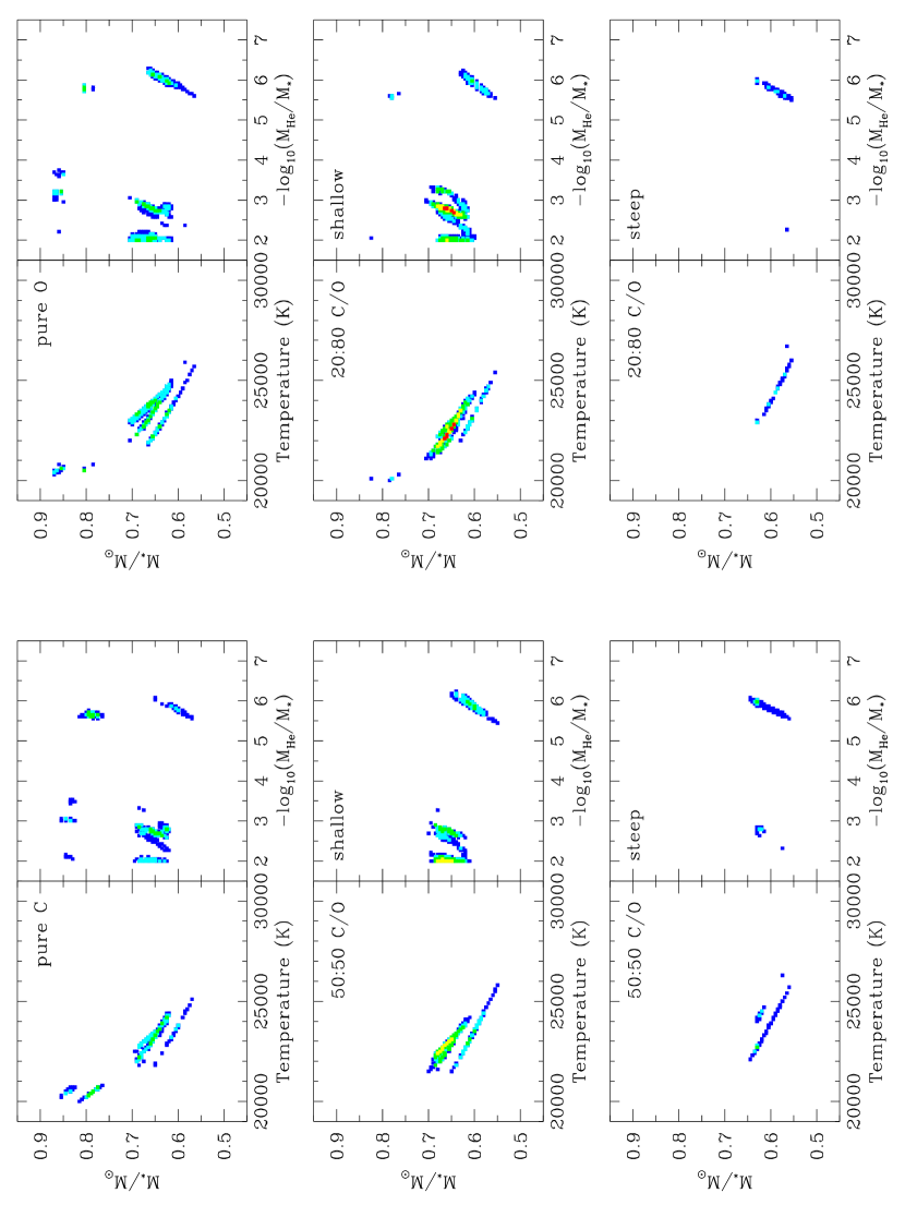
Figure 2: The families of models found by the GA which yield good matches to the periods observed in GD 358 for various core compositions and transition profiles. The quality of the fit is indicated by the color of the square: ${\rm r.m.s.}<3.0$ seconds (blue), $<2.75$ seconds (cyan), $<2.5$ seconds (green), $<2.0$ seconds (yellow), and $<1.65$ seconds (red).

Table 2

Results for GD 358 Data

	Best-fit Models
Core Composition	$T_{\rm eff}$	$M/M_{\odot}$	$\log(M_{\rm He}/M_{*})$	r.m.s.
pure C	20,300	0.795	$-$5.66	2.17a
	23,100	0.655	$-$2.74	2.30
50:50 C/O “shallow”$\ldots$	22,800	0.665	$-$2.00	1.76
	23,100	0.610	$-$5.92	2.46
50:50 C/O “steep”	22,700	0.630	$-$5.97	2.42
	24,300	0.625	$-$2.79	2.71
20:80 C/O “shallow”$\ldots$	22,600	0.650	$-$2.74	1.50b
	23,100	0.605	$-$5.97	2.48
20:80 C/O “steep”	22,900	0.630	$-$5.97	2.69
	27,300	0.545	$-$2.16	2.87a
pure O	20,500	0.805	$-$5.76	2.14a
	23,400	0.655	$-$2.79	2.31

^a Luminosity is inconsistent with observations

^b Best-fit solution

in GD 358 (Montgomery & Winget, 2000) by investigating whether ³He/⁴He/C/O models provide significantly better fits than these ⁴He-only models.

We have seen the first indications that our models of white dwarf stars are incomplete. We hope to identify and correct these weaknesses in the models by tackling the problem in reverse. Now that we have an objective global best-fit model, we can investigate what changes to the internal structure of the model (parameterized by the Brunt-Väisälä frequency) lead to even better fits than are possible with the current generation of models. This may lead us to identify regions of the interior where an improved knowledge of the constitutive physics would be most useful.

References

- Beauchamp et al. (1999) Beauchamp, A., Wesemael, F., Bergeron, P., Fontaine, G., Saffer, R. A., Liebert, J. & Brassard, P. 1999, ApJ, 516, 887
- Bern & Wramdemark (1973) Bern, K. & Wramdemark, S. 1973, Lowell Obs. Bull., No. 161
- Böhm & Cassinelli (1971) Böhm, K. H. & Cassinelli, J. 1971, A&A, 12, 21
- Bradley (1993) Bradley, P. 1993, Ph.D. thesis, University of Texas-Austin
- Bradley & Winget (1994a) Bradley, P. A. & Winget, D. E. 1994, ApJ, 421, 236
- Bradley & Winget (1994b) Bradley, P. A. & Winget, D. E. 1994, ApJ, 430, 850
- Bradley Winget & Wood (1993) Bradley, P. A., Winget, D. E. & Wood, M. A. 1993, ApJ, 406, 661
- Brassard Fontaine Wesemael & Hansen (1992) Brassard, P., Fontaine, G., Wesemael, F. & Hansen, C. J. 1992, ApJS, 80, 369
- Buchman (1996) Buchman, L. 1996, ApJ, 468, L127
- Charbonneau (1995) Charbonneau, P. 1995, ApJS, 101, 309
- Darwin (1859) Darwin, C. 1859, The Origin of Species (New York: Penguin Books)
- Dehner & Kawaler (1995) Dehner, B. T. & Kawaler, S. D. 1995, ApJ, 445, L141
- Fontaine Graboske & Van Horn (1977) Fontaine, G., Graboske, H. C., Jr., & Van Horn, H. M. 1977, ApJS, 35, 293
- Geist et al. (1994) Geist, A., Beguelin, A., Dongarra, J., Jiang, W., Manchek, R., & Sunderam, V. 1994, PVM: Parallel Virtual Machine, A Users’ Guide and Tutorial for Networked Parallel Computing, (Cambridge: MIT Press)
- Greenstein (1969) Greenstein, J. L. 1969, ApJ, 158, 281
- Harrington et al. (1985) Harrington, R. S. et al. 1985, AJ, 90, 123
- Iglesias & Rogers (1993) Iglesias, C. A., & Rogers, F. J. 1993, ApJ, 412, 752
- Itoh et al. (1989) Itoh, N., Adachi, T., Nakagawa, M., Kohyama, Y. & Munakata, H. 1989, ApJ, 339, 354
- Kawaler (1986) Kawaler, S. 1986, Ph.D. thesis, University of Texas-Austin
- Kawaler (1990) Kawaler, S. D. 1990, ASP Conf. Ser. 11: Confrontation Between Stellar Pulsation and Evolution, 494
- Kawaler & Weiss (1990) Kawaler, S. & Weiss, P. 1990, in Proc. Oji International Seminar, Progress of Seismology of the Sun and Stars, ed. Y. Osaki & H. Shibahashi (Berlin: Springer), 431
- Kutter & Savedoff (1969) Kutter, G. S. & Savedoff, M. P. 1969, ApJ, 156, 1021
- Lamb (1974) Lamb, D. Q. 1974, Ph.D. thesis, University of Rochester
- Lamb & van Horn (1975) Lamb, D. Q. & Van Horn, H. M. 1975, ApJ, 200, 306
- Metcalfe (1999) Metcalfe, T. S. 1999, AJ, 117, 2503
- Metcalfe & Nather (1999a) Metcalfe, T. S., & Nather, R. E. 1999a, Linux Journal, 65, 58
- Metcalfe & Nather (1999b) Metcalfe, T. S., & Nather, R. E. 1999b, Baltic Astronomy, 8, in press
- Montgomery (1998) Montgomery, M. H. 1998, Ph.D. thesis, University of Texas-Austin
- Montgomery & Winget (1999) Montgomery, M. H. & Winget, D. E. 1999, ApJ, 526, 976
- Montgomery & Winget (2000) Montgomery, M. H. & Winget, D. E. 2000, Baltic Astronomy, 8, in press
- Nather et al. (1990) Nather, R. E., Winget, D. E., Clemens, J. C., Hansen, C. J. & Hine, B. P. 1990, ApJ, 361, 309
- Napiwotzki Green & Saffer (1999) Napiwotzki, R., Green, P. J. & Saffer, R. A. 1999, ApJ, 517, 399
- Salaris et al. (1997) Salaris, M., Dominguez, I., Garcia-Berro, E., Hernanz, M., Isern, J. & Mochkovitch, R. 1997, ApJ, 486, 413
- Sweigart Greggio & Renzini (1990) Sweigart, A., Greggio, L. & Renzini, A. 1990, ApJ, 364, 527
- Vuille et al. (2000) Vuille, F. et al. 2000, MNRAS, 314, 689
- Wegner (1979) Wegner, G. 1979, in IAU Colloquium 53, White Dwarfs and Variable Degenerate Stars (Rochester, New York: University of Rochester), 250
- Winget (1981) Winget, D. E. 1981, Ph.D. thesis, University of Rochester
- Winget Robinson Nather & Fontaine (1982) Winget, D. E., Robinson, E. L., Nather, R. D. & Fontaine, G. 1982, ApJ, 262, L11
- Winget et al. (1991) Winget, D. E., et al. 1991, ApJ, 378, 326
- Winget et al. (1994) Winget, D. E., et al. 1994, ApJ, 430, 839
- Wood (1990) Wood, M. 1990, Ph.D. thesis, University of Texas-Austin