Launching of jets and the vertical structure of accretion disks

Abstract

The launching of magnetohydrodynamic outflows from accretion disks is considered. We formulate a model for the local vertical structure of a thin disk threaded by a poloidal magnetic field of dipolar symmetry. The model consists of an optically thick disk matched to an isothermal atmosphere. The disk is supposed to be turbulent and possesses an effective viscosity and an effective magnetic diffusivity. In the atmosphere, if the magnetic field lines are inclined sufficiently to the vertical, a magnetocentrifugal outflow is driven and passes through a slow magnetosonic point close to the surface. We determine how the rate of mass loss varies with the strength and inclination of the magnetic field. In particular, we find that for disks in which the mean poloidal field is sufficiently strong to stabilize the disk against the magnetorotational instability, the mass loss rate decreases extremely rapidly with increasing field strength, and is maximal at an inclination angle of 40–50^∘. For turbulent disks with weaker mean fields, the mass loss rate increases monotonically with increasing strength and inclination of the field, but the solution branch terminates before achieving excessive mass loss rates. Our results suggest that efficient jet launching occurs for a limited range of field strengths, and a limited range of inclination angles in excess of 30^∘. In addition, we determine the direction and rate of radial migration of the poloidal magnetic flux, and discuss whether configurations suitable for jet launching can be maintained against dissipation.

1. Introduction

Jets and other outflows are commonly observed from young stellar objects, interacting binary stars and active galactic nuclei. It is generally believed that the outflows are produced by the accretion disks in these systems. The widely differing properties of the central objects in these systems suggest that a mechanism may be at work that is largely independent of the nature of the central object (e.g. Livio 1997).

A particularly promising mechanism for the acceleration and collimation of outflows involves a large-scale poloidal magnetic field that threads the disk. The influential model of Blandford & Payne (1982) established the significance of the angle of inclination, $i$, of the poloidal magnetic field lines to the vertical at the surface of the disk. When $i>30^{\circ}$, matter that is just above the surface, being forced to corotate with the foot-point of the field line, is accelerated outwards along it by the centrifugal force. At greater distances, the flow may collimate into a jet by magnetic hoop stresses or poloidal collimation. A clear review of the physics of magnetocentrifugally driven outflows has been given by Spruit (1996).

Several groups have performed axisymmetric numerical simulations of outflows using this mechanism (e.g. Ustyugova et al. 1995; Romanova et al. 1997; Ustyugova et al. 1999; Ouyed & Pudritz 1997a, 1997b, 1999; Krasnopolsky, Li, & Blandford 1999). Like the model of Blandford & Payne (1982), these calculations do not resolve the vertical structure of the disk but treat it as a boundary surface that loads mass at a specified rate on to the magnetic field lines. While these simulations have convincingly demonstrated some aspects of the magnetocentrifugal model of jet production, several fundamental issues remain to be resolved. In this paper, we will attempt to address two of these questions. First, what determines the rate of mass loss in the outflow? How does this depend on the strength and inclination of the magnetic field, or on other properties of the disk? Second, what is the long-term evolution of a large-scale magnetic field in a disk? Is it possible to assemble a magnetic configuration suitable for jet launching, or to maintain it against dissipation? A proper understanding of these issues is essential if we are to explain the conditions that regulate the production of astrophysical jets.

The magnetocentrifugal mechanism can explain the acceleration of outflows even when the matter is ‘cold’ in the sense that the temperature is much less than the virial temperature or escape temperature. However, as mentioned by Blandford & Payne (1982) and calculated in detail by Ogilvie (1997) and by Ogilvie & Livio (1998; hereafter Paper I), some amount of thermal assistance is still required to overcome the potential barrier between the surface and the slow magnetosonic point (‘sonic point’). The barrier occurs because the field lines are not straight inside the disk and the angular velocity deviates slightly from the Keplerian value because of the radial Lorentz force associated with the bending of the field lines (Shu 1991; Wardle & Königl 1993). A proper calculation of the vertical structure of the disk, including these effects, is therefore required in order to determine the height of the potential barrier and the rate of mass loss in the outflow. Indeed, it is obvious from the well-known properties of transonic outflows that the mass loss rate depends on the physical conditions below the sonic point, and that the vertical structure must therefore be resolved.

In Paper I we carried out such a calculation for disks that are rather strongly magnetized in the sense that the magnetorotational instability, which leads to turbulence in accretion disks (Balbus & Hawley 1998), is suppressed or nearly so. We assumed that the magnetic field enforces strict isorotation and showed that the potential barrier increases very steeply as the field is made stronger and the disk becomes more sub-Keplerian. This effect would suppress outflows from strongly magnetized disks unless an additional source of energy, such as coronal heating, were present (in accord with the suggestion made by Livio 1997).

A disadvantage of the calculation in Paper I is that no explanation was given for the source of the effective viscosity of a disk in which the magnetorotational instability is suppressed. The solutions did not extend to field strengths much below the stability boundary. When the field is weaker than this, it cannot be expected to enforce isorotation, and the model requires some modification. In addition, the effect of the turbulence on the mean magnetic field should be modeled, most simply through the introduction of an effective magnetic diffusivity.

However, the presence of a turbulent diffusivity may cause problems for the magnetocentrifugal mechanism. The analysis by Lubow, Papaloizou, & Pringle (1994a) suggests that, if the effective magnetic Prandtl number of the disk is of order unity, as might be expected, it is impossible to sustain a steady configuration with a significantly inclined field in a thin disk (see also Heyvaerts, Priest, & Bardou 1996; Reyes-Ruiz & Stepinski 1996). Although the accretion flow tends to drag magnetic flux inwards, the turbulent diffusivity expels flux faster if the inclination is large. The inclination angle in a steady state is then expected to be comparable to the angular semi-thickness $H/r$ of the disk. This constraint can be avoided if the accretion flow is due primarily to the loss of angular momentum in an outflow, and might also be relieved by a dynamo operating in the disk if special conditions are met (Campbell, Papaloizou, & Agapitou 1998).

The purpose of the present paper is to explore a model for the vertical structure of magnetized disks. We will extend the analysis of Paper I to allow for the possibility of more weakly magnetized disks in which there is turbulence, and strict isorotation does not hold. We will also give a better treatment of the matching between the disk and the atmosphere by applying photospheric boundary conditions, allowing us to calculate the mass loss rate in the outflow explicitly. At the same time, we will solve for the rate of dragging of magnetic flux and thereby refine the previous estimates which may have been based on oversimple arguments.

Related calculations of the vertical structure of magnetized disks, and of the disk-jet connection, have been made by Königl (1989), Wardle & Königl (1993), Li (1995, 1996), Ferreira (1997), Campbell (1999), Casse & Ferreira (2000), and Shalybkov & Rüdiger (2000). Our method and results are significantly different from all previous calculations and comparisons of the relevant issues will be made towards the end of this paper.

2. Context of the present calculation

To set this calculation in its proper context, we consider here some of the wider issues relating to magnetized accretion disks and outflows.

For a thin disk without a large-scale magnetic field, there is a clear division of the physical problem into two aspects. First, a model is required for the local vertical structure at any given radius $r$ and time $t$. Such a model takes the surface mass density $\Sigma$ as a parameter and predicts quantities such as the vertically integrated viscous stress ${\cal G}$. The vertical structure may be assumed to be stationary on the dynamical time-scale. Second, the one-dimensional conservation equations for mass and angular momentum determine how $\Sigma(r,t)$ evolves on the viscous time-scale, given the local relation between ${\cal G}$ and $\Sigma$ (e.g. Lynden-Bell & Pringle 1974).

For a disk with a large-scale poloidal magnetic field but no outflows (e.g. a polytrope with a force-free or vacuum exterior), the situation is similar but more complicated. Now the local vertical structure at a given radius depends not only on $\Sigma$ but also on the vertical magnetic field $B_{z}$ and the inclination angle $i$. In addition to an evolutionary equation for $\Sigma$, there is a one-dimensional conservation equation for magnetic flux, which determines how the flux function $\psi(r,t)$ evolves on the viscous time-scale. $B_{z}$ is simply related to the radial derivative of $\psi$. Finally, the force-free magnetic equilibrium in the exterior of the disk leads to a global relation between $\psi$ and the inclination angle $i$. The full problem therefore involves an integro-differential equation. This has been considered by Lubow et al. (1994a), although they did not examine the effect of the magnetic field on the vertical disk structure.

When outflows occur along the magnetic field lines, further couplings exist. The exterior magnetic field is modified from the force-free solution by the inertial forces associated with the outflow. This effect depends on the amount of mass loading, and is therefore coupled to the launching problem. The exterior field is no longer purely poloidal but becomes significantly twisted beyond the Alfvén surface, although non-axisymmetric (e.g. kink) instabilities may set in here (e.g. Spruit, Foglizzo, & Stehle 1997). This part of the solution is established on the Alfvén travel time to the Alfvén surface, which is comparable to the dynamical time-scale of the disk. Finally, the mass loss and especially the angular momentum loss in the outflow feed back into the evolutionary equations for the disk.

The full problem therefore involves three aspects: the local vertical structure of the disk and the launching problem; the global structure of the exterior magnetic field and the dynamics of the outflow along those field lines; and the evolution of mass, angular momentum, and magnetic flux on a longer time-scale. The first aspect is the subject of this paper, while the second aspect is well described by some of the numerical simulations referred to above. The third aspect has been considered implicitly in steady models such as that of Casse & Ferreira (2000), but the development of a complete evolutionary scheme for mass, angular momentum and magnetic flux in the general, non-steady case remains a challenge (see Lovelace, Newman, & Romanova 1997 for a simplified version of such a scheme).

There has been some confusion in the literature regarding the interplay between these aspects of the problem. For example, studies of the launching problem have often imposed the condition that the poloidal magnetic flux should not migrate radially (e.g. Königl 1989; Li 1995). That is, there should be an instantaneous balance between inward advection of flux by the accretion flow, and outward transport due to turbulent, Ohmic, or ambipolar diffusion. This may not always be appropriate because the migration occurs on the viscous time-scale, whereas the solution of the launching problem need only be stationary on the dynamical time-scale. In Wardle & Königl (1993) the rate of flux migration was treated as a free parameter.

Moreover, some of these studies appear to predict the value of the toroidal magnetic field at the surface of the disk, $B_{\phi{\rm s}}$, even when the dynamics of the outflow beyond the sonic point has not been considered (e.g. Campbell 1999) or when there is no outflow (e.g. Shalybkov & Rüdiger 2000). This is unsatisfactory because $B_{\phi{\rm s}}$ determines the external magnetic torque acting on the disk, which certainly depends on the dynamics of the outflow in the trans-Alfvénic region. These incorrectly specified studies may be motivated by the fact that the model of Blandford & Payne (1982) appears to require $B_{\phi{\rm s}}$ to be determined by the disk (through their parameter $\lambda$). However, this is misleading and may be attributed to the fact that the Blandford & Payne model is underconstrained because it is missing a boundary condition at large distances from the disk (cf. Ostriker 1997). Indeed, solutions of their model generically behave unphysically at large distances without having passed through the modified fast magnetosonic point. In contrast, Krasnopolsky et al. (1999) have given a clear discussion of which quantities may or may not be specified as boundary conditions when treating the disk as a boundary surface. In their model $B_{\phi{\rm s}}$ is determined by the outflow, not by the disk.

In our local study, therefore, we will not impose the constraint of zero flux migration; rather, we will impose the value of $B_{\phi{\rm s}}$ and determine the rate of flux migration. Usually we will specify $B_{\phi{\rm s}}=0$, meaning that the outflow is absent or exerts only a weak torque. Efficient magnetocentrifugal outflows are expected to have $|B_{\phi{\rm s}}|\ll|B_{z}|$, with the toroidal field becoming comparable to the poloidal component only at greater distances from the source, where the Alfvén surface is located (Spruit 1996).

3. The evolution of magnetic flux

As noted above, an important investigation of the evolution of the poloidal magnetic flux was made by Lubow et al. (1994a), who concluded that, if the disk is turbulent, with an effective magnetic Prandtl number of order unity, the accretion flow will be almost entirely ineffective in dragging in magnetic flux. This can be explained by noting that the effective magnetic Reynolds number of the accretion flow, based on the disk thickness $H$, is small, of order $H/r$ (Heyvaerts et al. 1996). Similar arguments suggest that a configuration in which the field lines are bent significantly from the vertical (e.g. to achieve $i>30^{\circ}$) cannot be sustained on the viscous time-scale.

These arguments are based on a kinematic analysis of the magnetic induction equation in which the radial velocity and magnetic diffusivity are prescribed quantities. They also depend on a simple order-of-magnitude treatment of the vertical structure of the magnetic field. In this paper we will present a numerical treatment of a set of equations, including the induction equation, in which the radial velocity is self-consistently determined. This is important because, in a jet-launching configuration, the magnetic field must become dynamically dominant above some height and will then control the radial velocity. We will find results that differ significantly from the estimates of Lubow et al. (1994) under some circumstances. Before presenting the numerical model, we therefore reconsider the problem of the induction equation from an analytical viewpoint.

We assume that the mean poloidal magnetic field is axisymmetric and may be described by a flux function $\psi(r,z,t)$ such that

$$B_{r}=-{{1}\over{r}}{{\partial\psi}\over{\partial z}},\qquad B_{z}={{1}\over{r}}{{\partial\psi}\over{\partial r}}.$$ (1)

For a thin disk containing a bending poloidal field of dipolar symmetry, the flux function has the form (Ogilvie 1997)

$$\psi=\psi_{0}(r,t)+\psi_{1}(r,z,t),$$ (2)

where $|\psi_{1}|\ll|\psi_{0}|$. Then $B_{r}$ and $B_{z}$ are comparable in magnitude if $|\psi_{1}/\psi_{0}|=O(H/r)$. The flux content of the disk is determined essentially by $\psi_{0}$, while $\psi_{1}$ allows for bending of the field lines within the disk.

We assume that the mean magnetic field in a turbulent disk may be treated within the framework of mean-field electrodynamics (e.g. Moffatt 1978). In the absence of a mean-field dynamo effect (or in the absence of a toroidal field), the flux function then satisfies the mean induction equation,

$${{\partial\psi}\over{\partial t}}+\mbox{\boldmath$u$}\!\cdot\!\nabla\psi=\eta r^{2}\nabla\!\cdot\left({{1}\over{r^{2}}}\nabla\psi\right),$$ (3)

where $u$ is the mean velocity and $\eta$ the turbulent magnetic diffusivity. In a thin disk the dominant terms are

$${{\partial\psi_{0}}\over{\partial t}}+u_{r}{{\partial\psi_{0}}\over{\partial r}}=\eta r{{\partial}\over{\partial r}}\left({{1}\over{r}}{{\partial\psi_{0}}\over{\partial r}}\right)+\eta{{\partial^{2}\psi_{1}}\over{\partial z^{2}}}.$$ (4)

The neglected terms are all smaller than those retained because $|\psi_{1}|\ll|\psi_{0}|$ and $|u_{r}|\gg|u_{z}|$. The first term on the right-hand side is also sometimes neglected (e.g. Lubow et al. 1994a).

Although this equation appears to be an evolutionary equation for $\psi_{0}$ it should be observed that the equation is defined for all values of $z$ whereas $\psi_{0}$ is a function of $r$ and $t$ only. Moreover, the equation is not closed because of the term involving $\psi_{1}$. Following Lubow et al. (1994a), we might attempt to close the equation by vertical averaging. Conventionally in accretion-disk theory one uses density-weighted averages $\bar{u}_{r}$ and $\bar{\eta}$ defined by

$$\Sigma\bar{u}_{r}=\int\rho u_{r}\,{\rm d}z,\qquad\Sigma\bar{\eta}=\int\rho\eta\,{\rm d}z,$$ (5)

where $\rho$ is the density and

$$\Sigma=\int\rho\,{\rm d}z$$ (6)

is the surface density, the integrals being over the full vertical extent of the disk. The density-weighted average $\bar{u}_{r}$ is particularly appropriate because it is directly related to the mass accretion rate. The vertical average of the induction equation is then

$${{\partial\psi_{0}}\over{\partial t}}+\bar{u}_{r}{{\partial\psi_{0}}\over{\partial r}}=\bar{\eta}r{{\partial}\over{\partial r}}\left({{1}\over{r}}{{\partial\psi_{0}}\over{\partial r}}\right)-{{r}\over{\Sigma}}\int\rho\eta{{\partial B_{r}}\over{\partial z}}\,{\rm d}z.$$ (7)

Lubow et al. proceeded by approximating the last term as $-(r/H)\bar{\eta}B_{r{\rm s}}$. This closes the equation because $B_{r{\rm s}}$, which is proportional to the vertically integrated toroidal electric current, can be globally related to the flux function by considering the force balance exterior to the disk. If the exterior region is treated either as an insulating vacuum, or as a force-free medium with vanishing $B_{\phi}$, the exterior poloidal field is potential. This leads to a global relation of the form

$$B_{r{\rm s}}={\cal L}^{-1}\psi_{0},$$ (8)

where ${\cal L}$ is a certain linear integral operator (see also Ogilvie 1997).

This order-of-magnitude estimate of the final term appears reasonable if the field lines bend mainly in the densest layers of the disc near the midplane. However, the term might be significantly overestimated if the bending occurs mainly in the upper layers of the disk where $\rho\eta$ is likely to be considerably smaller. Another way of averaging the induction equation reinforces this concern. If the equation is divided by $\eta$ and integrated with respect to $z$, we obtain

$${{\partial\psi_{0}}\over{\partial t}}+u_{*}{{\partial\psi_{0}}\over{\partial r}}=\eta_{*}r{{\partial}\over{\partial r}}\left({{1}\over{r}}{{\partial\psi_{0}}\over{\partial r}}\right)-QB_{r{\rm s}},$$ (9)

where

$$u_{*}(r,t)=\int{{u_{r}}\over{\eta}}\,{\rm d}z\bigg{/}\int{{1}\over{\eta}}\,{\rm d}z,$$ (10)

$$\eta_{*}(r,t)=\int{\rm d}z\bigg{/}\int{{1}\over{\eta}}\,{\rm d}z,$$ (11)

and

$$Q(r,t)=2r\bigg{/}\int{{1}\over{\eta}}\,{\rm d}z.$$ (12)

Now the precise shape of the field line has truly been eliminated in favor of $B_{r{\rm s}}$. This therefore appears to be the ‘correct’ way of averaging the equation. However, we are now faced with vertical averages of $u_{r}$ and $\eta$ weighted by $1/\eta$, not by $\rho$. Even if $\eta$ is independent of $z$, these could be significantly different from the density-weighted averages, leading to different conclusions about flux dragging.

Furthermore, as mentioned above, the presence of the magnetic field will in general change the vertical profiles of $u_{r}$ and $\eta$. If the field is extremely weak so that the induction equation may be treated ‘kinematically’, then the $1/\eta$ averaging method is surely the correct one. However, the vertical profile of $u_{r}$, in particular, is determined by subtle effects (e.g. Kley & Lin 1992) and is easily distorted by even weak Lorentz forces. In this case we cannot obtain a closed equation because $u_{*}$ cannot be determined from a knowledge of the mass accretion rate. The essential difficulty is that, while $\bar{u}_{r}$ is the relevant mean velocity for mass accretion, $u_{*}$ is the appropriate mean for flux accretion. These could be significantly disparate and could even differ in sign. The above discussion shows that the only solution to this problem is to solve explicitly for the vertical structure of the disk including the physics that determines the vertical profile of the radial velocity.

4. Mathematical model

We now consider the set of equations governing the local vertical structure of a disk containing a mean poloidal magnetic field. The equations of Paper I will be augmented by the inclusion of additional physical effects.

4.1. Basic equations for a thin disk

The angular velocity is written as

$$\Omega=\Omega_{0}(r)+\Omega_{1}(r,z,t),$$ (13)

where

$$\Omega_{0}=\left({{GM}\over{r^{3}}}\right)^{1/2}$$ (14)

is the Keplerian value, and $|\Omega_{1}|\ll\Omega_{0}$.

The flux function is written as

$$\psi=\psi_{0}(r,t)+\psi_{1}(r,z,t),$$ (15)

where $|\psi_{1}|\ll|\psi_{0}|$, and we approximate

$$B_{r}=-{{1}\over{r}}{{\partial\psi_{1}}\over{\partial z}},\qquad B_{z}\approx{{1}\over{r}}{{\partial\psi_{0}}\over{\partial r}},$$ (16)

so that $B_{z}$ is independent of $z$.

The required equations may be approximated as follows. The radial component of the equation of motion is

$$-2\rho r\Omega_{0}\Omega_{1}={{B_{z}}\over{\mu_{0}}}{{\partial B_{r}}\over{\partial z}},$$ (17)

where $\mu_{0}$ is the permeability of free space. The azimuthal component is

$${{\rho u_{r}}\over{r}}{{d}\over{dr}}(r^{2}\Omega_{0})={{B_{z}}\over{\mu_{0}}}{{\partial B_{\phi}}\over{\partial z}}+{{1}\over{r^{2}}}{{\partial}\over{\partial r}}\left(\rho\nu r^{3}{{d\Omega_{0}}\over{dr}}\right),$$ (18)

where $\nu$ is the kinematic viscosity. The vertical component is

$$0=-\rho\Omega_{0}^{2}z-{{\partial}\over{\partial z}}\left(p+{{B_{r}^{2}}\over{2\mu_{0}}}+{{B_{\phi}^{2}}\over{2\mu_{0}}}\right),$$ (19)

where $p$ is the pressure. The poloidal part of the induction equation is

$${{\partial\psi_{0}}\over{\partial t}}+ru_{r}B_{z}=r\eta\left({{\partial B_{z}}\over{\partial r}}-{{\partial B_{r}}\over{\partial z}}\right).$$ (20)

The toroidal part is

$$0=r\left(B_{r}{{d\Omega_{0}}\over{dr}}+B_{z}{{\partial\Omega_{1}}\over{\partial z}}\right)+{{\partial}\over{\partial z}}\left(\eta{{\partial B_{\phi}}\over{\partial z}}\right).$$ (21)

The energy equation is

$${{\partial F}\over{\partial z}}=\rho\nu\left(r{{d\Omega_{0}}\over{dr}}\right)^{2}+{{\eta}\over{\mu_{0}}}\left[\left({{\partial B_{r}}\over{\partial z}}\right)^{2}+\left({{\partial B_{\phi}}\over{\partial z}}\right)^{2}\right],$$ (22)

where

$$F=-{{16\sigma T^{3}}\over{3\kappa\rho}}{{\partial T}\over{\partial z}}$$ (23)

is the radiative energy flux, with $\sigma$ the Stefan-Boltzmann constant, $T$ the temperature, and $\kappa$ the Rosseland mean opacity.

These equations must be supplemented by constitutive relations specifying the equation of state, the opacity, the viscosity, and the magnetic diffusivity. We will adopt the ideal-gas equation of state,

$$p={{k\rho T}\over{\mu m_{\rm H}}},$$ (24)

(where $k$ is the Boltzmann constant, $\mu$ the mean molecular mass, and $m_{\rm H}$ the mass of the hydrogen atom), and a generic power-law opacity,

$$\kappa=C_{\kappa}\rho^{x}T^{y},$$ (25)

where $C_{\kappa}$, $x$, and $y$ are constants. This includes the cases of Thomson scattering opacity ($x=y=0$) and Kramers opacity ($x=1$, $y=-7/2$).

4.2. Turbulent viscosity and magnetic diffusivity

The viscosity is less certain, and we will adopt the standard prescription

$$\rho\nu={{\alpha p}\over{\Omega_{0}}},$$ (26)

where $\alpha$ is a dimensionless constant. For the magnetic diffusivity, we assume that the magnetic Prandtl number,

$${\rm Pm}={{\nu}\over{\eta}},$$ (27)

is constant.

We will further assume either that $\alpha$ is a fixed parameter (‘fixed alpha hypothesis’), or that $\alpha$ can adjust so as to keep the equilibrium at marginal magnetorotational stability, as explained in Section 4.8 below (‘marginal stability hypothesis’).

4.3. Neglected terms

Several terms in the equations have been omitted on the grounds that the disk is thin and the solution should be stationary on the dynamical time-scale (although not necessarily on the viscous time-scale). The radial pressure gradient, the vertical variation of radial gravity, and the inertial terms associated with the meridional flow, have been neglected as usual. However, enough terms have been retained to determine the profile of radial velocity in the absence of a magnetic field.

Generally, $\Omega_{1}$ has been neglected relative to $\Omega_{0}$, and $\psi_{1}$ relative to $\psi_{0}$, except where physically essential. It has also been assumed that the viscosity does not act on the shear components $\partial u_{r}/\partial z$ and $r\partial\Omega_{1}/\partial z$. Such terms are expected to be relatively unimportant in most cases of interest, and it was found that the inclusion of these terms increases the order of the differential system and makes it difficult to obtain a solution. It is especially unclear how to connect a viscous disk to an inviscid atmosphere, when these terms are included, without introducing an artificial boundary layer.

We did not include a dynamo alpha-effect in the equations for the mean magnetic field. Although there is no difficulty in principle in doing so, this effect is even less well understood than the turbulent viscosity and magnetic diffusivity, and we chose to avoid this additional complication in the present study.

Finally, in the energy equation (22) it has been assumed that the heat generated in each annulus is radiated away locally and not advected through the disk.

4.4. Local and non-local effects

The equations of Section 4.1 describe the local vertical structure of an accretion disk with a mean poloidal magnetic field. When supplemented with appropriate boundary conditions, as described below, they constitute a problem similar in type to a stellar structure calculation, although the details are of course very different. Obviously it is possible in principle to include a more detailed equation of state, accurate opacity tables, a more sophisticated approach to radiative transfer, and further possibilities such as convective energy transport. However, the principal uncertainties concern the viscosity and magnetic diffusivity.

In fact, these equations are not strictly local in radius and time because some radial derivatives and one time-derivative remain. The case of $d\Omega_{0}/dr=-3\Omega_{0}/2r$ is trivial. The terms $\partial\psi_{0}/\partial t$ and $\partial B_{z}/\partial r$ in the poloidal part of the induction equation are retained in order to determine whether the magnetic flux migrates inwards ($\partial\psi_{0}/\partial t>0$) or outwards as a result of the local disk solution. The gradient $\partial B_{z}/\partial r$ can affect this result because it contributes to the diffusion of flux. Therefore $\partial B_{z}/\partial r$ appears as a parameter of the local model and $\partial\psi_{0}/\partial t$ as an eigenvalue; note that both are independent of $z$.

The case of $\partial(\rho\nu)/\partial r$ is more problematic. This viscous term is retained in the angular momentum equation because it partially determines the radial velocity, which in turn causes radial advection of magnetic flux and also affects the shape of the field lines, at least when the field is weak. This term may be approximated by arguing that

$$\rho\nu\approx{{\bar{\nu}\Sigma}\over{H}}f\left({{z}\over{H}}\right)$$ (28)

in the neighborhood of the radius under consideration, where

$$\bar{\nu}\Sigma=\int_{-H}^{H}\rho\nu\,dz$$ (29)

is the vertically integrated dynamic viscosity, $H$ the semi-thickness, and $f$ an undetermined dimensionless function. Under this assumption,

$${{\partial\ln(\rho\nu)}\over{\partial\ln r}}={{\partial\ln(\bar{\nu}\Sigma)}\over{\partial\ln r}}-\left[1+{{\partial\ln(\rho\nu)}\over{\partial\ln z}}\right]{{\partial\ln H}\over{\partial\ln r}}.$$ (30)

The vertical derivative is available as part of the local solution, while $\partial\ln(\bar{\nu}\Sigma)/\partial\ln r$ and $\partial\ln H/\partial\ln r$ appear as additional dimensionless parameters, which can be estimated from the well-known behavior of the steady, non-magnetized solution (Shakura & Sunyaev 1973).

In the limit of a non-magnetized disk, this prescription predicts the radial velocity in the disk as

$$u_{r}=-{{3\nu}\over{2r}}\left\{1+2{{\partial\ln(\bar{\nu}\Sigma)}\over{\partial\ln r}}-2\left[1+{{\partial\ln(\rho\nu)}\over{\partial\ln z}}\right]{{\partial\ln H}\over{\partial\ln r}}\right\}.$$ (31)

4.5. Boundary conditions

We have derived a sixth-order system of nonlinear ordinary differential equations (ODEs) in $z$. The dependent variables may be taken as $p$, $T$, $F$, $\Omega_{1}$, $B_{r}$, and $B_{\phi}$. The variables $\rho$ and $u_{r}$ are determined algebraically from these.

The solution should be symmetric about the mid-plane, with

$$F=B_{r}=B_{\phi}=0$$ (32)

at $z=0$.

The solution extends up to a photospheric surface $z=H$ at which it is matched to a simple atmospheric model, discussed below. The photospheric boundary conditions are

$$F_{\rm s}=\sigma T_{\rm s}^{4}$$ (33)

and

$$\tau_{\rm s}=\int_{H}^{\infty}\kappa\rho\,dz={{2}\over{3}},$$ (34)

where the subscript ‘s’ denotes a surface value. We also have

$$B_{r}=B_{r{\rm s}},\qquad B_{\phi}=B_{\phi{\rm s}}$$ (35)

there, where $B_{r{\rm s}}$ and $B_{\phi{\rm s}}$ are assigned values which, physically, are determined by the solution of the global exterior outflow problem (not considered here).

With these boundary conditions the equation of angular momentum conservation, obtained from a vertical integration of equation (18), has the form

$$-{{\dot{M}}\over{2\pi r^{2}}}{{d}\over{dr}}(r^{2}\Omega_{0})={{2B_{z}B_{\phi{\rm s}}}\over{\mu_{0}}}+{{1}\over{r^{2}}}{{\partial}\over{\partial r}}\left(\bar{\nu}\Sigma r^{3}{{d\Omega_{0}}\over{dr}}\right),$$ (36)

where

$$\dot{M}=-2\pi r\int_{-H}^{H}\rho u_{r}\,dz$$ (37)

is the mass accretion rate, not necessarily constant. This shows the contributions to angular momentum transport from magnetic and viscous torques.

The solution is determined as follows. One guesses the values of the quantities $H$, $F_{\rm s}$, and $\Omega_{1{\rm s}}$. This fixes the atmospheric model and determines $p_{\rm s}$ and $T_{\rm s}$. The quantities $B_{r{\rm s}}$ and $B_{\phi{\rm s}}$ are given. One must further guess $\partial\psi_{0}/\partial t$ to start the downward integration. The three guessed quantities should be adjusted to match the three symmetry conditions on $z=0$. The main parameters of the model are then $\Omega_{0}$, $\Sigma$, $B_{z}$, $B_{r{\rm s}}$, $B_{\phi{\rm s}}$, $\alpha$, and ${\rm Pm}$. The quantity $\partial\psi_{0}/\partial t$ is to be determined as an eigenvalue.

4.6. Atmospheric model

In the simplest atmospheric model, $T$, $F$, $B_{r}$, and $B_{\phi}$ are independent of $z$ between the photosphere and the sonic point, with

$$T = T_{\rm s}=T_{\rm eff},$$ (38)

$$F = F_{\rm s}=\sigma T_{\rm s}^{4},$$ (39)

$$B_{r} = B_{r{\rm s}}=B_{z}\tan i,$$ (40)

$$B_{\phi} = B_{\phi{\rm s}},$$ (41)

where $i$ is the inclination of the field lines to the vertical. The constancy of $F$ relies on there being little or no dissipation in the atmosphere, while the constancy of $B$ relies on the atmosphere being magnetically dominated so that field line bending cannot be supported. That is, the plasma beta based on the poloidal magnetic field strength,

$$\beta={{2\mu_{0}p}\over{B_{r}^{2}+B_{z}^{2}}},$$ (42)

should be less than unity.

In the atmosphere, all diffusive terms in the equations are neglected. If $\partial\psi_{0}/\partial t\neq 0$, there must be a slow drift orthogonal to the poloidal field lines, but otherwise the flow is constrained to follow the field. We know from Paper I that there will be a transonic outflow if $i>30^{\circ}$, otherwise a modified hydrostatic atmosphere.

As in Paper I, the angular velocity in the atmosphere is determined by isorotation,

$$\Omega_{1}=\Omega_{1{\rm s}}+{{3\Omega_{0}}\over{2r}}(z-H)\tan i.$$ (43)

Again, this assumes that the atmosphere is magnetically dominated. The centrifugal-gravitational potential for matter constrained to follow the field is

$$\Phi^{\rm cg}=-{{1}\over{2}}(3\tan^{2}i-1)\Omega_{0}^{2}(z-z_{\rm sonic})^{2},$$ (44)

where

$$z_{\rm sonic}=H\left[1+(3\tan^{2}i-1)^{-1}\left(1-2{{\Omega_{1{\rm s}}r}\over{\Omega_{0}H}}\tan i\right)\right]$$ (45)

is the height of the sonic point in the case $i>30^{\circ}$.

The density scale-height $h_{\rm s}$ at the photosphere is given by

$${{c_{\rm s}^{2}}\over{h_{\rm s}}}=\left({{\partial\Phi^{\rm cg}}\over{\partial z}}\right)_{\rm s}=\Omega_{0}^{2}H\left(1-2{{\Omega_{1{\rm s}}r}\over{\Omega_{0}H}}\tan i\right),$$ (46)

where $c_{\rm s}$ is the isothermal sound speed, given by

$$c_{\rm s}^{2}={{kT_{\rm s}}\over{\mu m_{\rm H}}}.$$ (47)

To a good approximation, the photospheric boundary condition (34) equates to

$${{2}\over{3}}=C_{\kappa}\rho_{\rm s}^{1+x}T_{\rm s}^{y}\int_{0}^{\infty}\exp\left[-(1+x)\left({{z-H}\over{h_{\rm s}}}\right)\right]\,d(z-H).$$ (48)

This may be rearranged into the form

$$\rho_{\rm s}^{1+x}T_{\rm s}^{1+y} = \left({{1+x}\over{8\sigma}}\right)\left({{\mu m_{\rm H}}\over{k}}\right)\left({{16\sigma}\over{3C_{\kappa}}}\right)\Omega_{0}^{2}H$$ (49)

$$\qquad\times\left(1-2{{\Omega_{1{\rm s}}r}\over{\Omega_{0}H}}\tan i\right).$$

Finally, in the case of a transonic outflow, the Mach number at the surface is determined from the equation (see Paper I)

$${{1}\over{2}}({\cal M}_{\rm s}^{2}-1)-\ln{\cal M}_{\rm s}={{\Delta\Phi}\over{c_{\rm s}^{2}}},$$ (50)

where

$$\Delta\Phi={{(\Omega_{0}H-2\Omega_{1{\rm s}}r\tan i)^{2}}\over{2(3\tan^{2}i-1)}}$$ (51)

is the potential barrier to the outflow. The vertical mass flux density in the outflow is then

$$\dot{m}_{\rm w}=\rho u_{z}={\cal M}_{\rm s}\rho_{\rm s}c_{\rm s}\cos i.$$ (52)

4.7. Non-dimensionalization

We now rewrite the equations in a non-dimensional form suitable for numerical analysis. Given the local surface density $\Sigma$, the angular velocity $\Omega_{0}$, and the constants appearing in the constitutive relations, we identify

$$U_{H} = \Sigma^{(2+x)/(6+x-2y)}\Omega_{0}^{-(5-2y)/(6+x-2y)}$$ (53)

$$\times\left({{\mu m_{\rm H}}\over{k}}\right)^{-(4-y)/(6+x-2y)}\left({{16\sigma}\over{3C_{\kappa}}}\right)^{-1/(6+x-2y)}$$

as a natural unit for the semi-thickness of the disk. Natural units for other physical quantities follow according to

$$U_{\rho}=\Sigma U_{H}^{-1},\qquad U_{p}=\Sigma\Omega_{0}^{2}U_{H},$$ (54)

$$U_{T}=\Omega_{0}^{2}\left({{\mu m_{\rm H}}\over{k}}\right)U_{H}^{2},\qquad U_{F}=\Omega_{0}U_{H}U_{p},$$ (55)

$$U_{B}=(\mu_{0}U_{p})^{1/2}.$$ (56)

Note that the above expression for $U_{H}$ can be obtained from the condition

$$U_{F}={{16\sigma U_{T}^{3}}\over{3C_{\kappa}U_{\rho}^{x}U_{T}^{y}U_{\rho}}}{{U_{T}}\over{U_{H}}},$$ (57)

which is a dimensional analysis of the definition (23) of the radiative flux.

There are two small dimensionless parameters in the problem,

$$\epsilon={{U_{H}}\over{r}},\qquad\delta={{U_{F}}\over{\sigma U_{T}^{4}}}.$$ (58)

Evidently $\epsilon$ is a characteristic measure of the angular semi-thickness of the disk, while $\delta$ is an inverse measure of the total optical thickness.

Non-dimensional variables are then introduced using the transformations

$$z=z_{*}\,U_{H},\qquad H=H_{*}\,U_{H},$$ (59)

$$\rho=\rho_{*}\,U_{\rho},\qquad p=p_{*}\,U_{p}$$ (60)

$$T=T_{*}\,U_{T},\qquad F=F_{*}\,U_{F},$$ (61)

$$\nu=\nu_{*}\,\Omega_{0}U_{H}^{2},\qquad\eta=\eta_{*}\,\Omega_{0}U_{H}^{2},$$ (62)

$$u_{r}=u_{r*}\,\Omega_{0}U_{H},\qquad\Omega_{1}=\Omega_{1*}\,\epsilon\Omega_{0},$$ (63)

$$B_{r}=B_{r*}\,U_{B},\qquad B_{\phi}=B_{\phi*}\,U_{B},$$ (64)

$$B_{z}=B_{z*}\,U_{B},\qquad{{\partial\psi_{0}}\over{\partial t}}=\dot{\psi}_{*}\,r\Omega_{0}U_{H}U_{B}.$$ (65)

The transformed equations are

$$-2\rho_{*}\Omega_{1*}=B_{z*}B_{r*}^{\prime},$$ (66)

$${{1}\over{2}}\rho_{*}u_{r*}=B_{z*}B_{\phi*}^{\prime}-{{3}\over{4}}\epsilon(1+2D_{\nu\Sigma})\rho_{*}\nu_{*}+{{3}\over{2}}\epsilon D_{H}(\rho_{*}\nu_{*}z_{*})^{\prime},$$ (67)

$$0=-\rho_{*}z_{*}-p_{*}^{\prime}-B_{r*}B_{r*}^{\prime}-B_{\phi*}B_{\phi*}^{\prime},$$ (68)

$$\dot{\psi}_{*}+u_{r*}B_{z*}=\eta_{*}\left(\epsilon D_{B}B_{z*}-B_{r*}^{\prime}\right),$$ (69)

$$0=-{{3}\over{2}}B_{r*}+B_{z*}\Omega_{1*}^{\prime}+(\eta_{*}B_{\phi*}^{\prime})^{\prime},$$ (70)

$$F_{*}^{\prime}={{9}\over{4}}\rho_{*}\nu_{*}+\eta_{*}\left[(B_{r*}^{\prime})^{2}+(B_{\phi*}^{\prime})^{2}\right],$$ (71)

$$F_{*}=-{{T_{*}^{3-y}}\over{\rho_{*}^{1+x}}}T_{*}^{\prime},$$ (72)

$$p_{*}=\rho_{*}T_{*},$$ (73)

where

$$D_{\nu\Sigma}={{\partial\ln(\bar{\nu}\Sigma)}\over{\partial\ln r}},\qquad D_{H}={{\partial\ln H}\over{\partial\ln r}},\qquad D_{B}={{\partial\ln B_{z}}\over{\partial\ln r}}$$ (74)

are three dimensionless parameters, and the prime denotes differentiation with respect to $z_{*}$.

The dimensionless viscosity and magnetic diffusivity are given by

$$\nu_{*}={\rm Pm}\,\eta_{*}=\alpha T_{*}.$$ (75)

The mid-plane symmetry conditions are

$$F_{*}(0)=B_{r*}(0)=B_{\phi*}(0)=0.$$ (76)

The photospheric boundary conditions are

$$\delta F_{*}(H_{*})=[T_{*}(H_{*})]^{4}$$ (77)

and

$$[\rho_{*}(H_{*})]^{1+x}[T_{*}(H_{*})]^{1+y}={{1}\over{8}}\delta(1+x)[H_{*}-2\Omega_{1*}(H_{*})\tan i],$$ (78)

together with

$$B_{r*}(H_{*})=B_{r{\rm s}*},\qquad B_{\phi*}(H_{*})=B_{\phi{\rm s}*}.\qquad$$ (79)

Finally, the definition of $\Sigma$ implies the normalization condition

$$2\int_{0}^{H_{*}}\rho_{*}\,dz_{*}=1.$$ (80)

When the solution is found, the optical depth at the mid-plane can be determined from

$$\tau_{\rm c}={{2}\over{3}}+\int_{0}^{H}\kappa\rho\,dz={{2}\over{3}}+{{16}\over{3\delta}}\int_{0}^{H_{*}}\rho_{*}^{1+x}T_{*}^{y}\,dz_{*}.$$ (81)

The fact that the small parameter $\epsilon$ cannot be fully scaled out of the equations indicates that a strictly self-consistent thin-disk asymptotic solution cannot be obtained when all the physical effects we have considered are included. The $\epsilon$ terms in equation (67) are expected to be important only in the case of a weak magnetic field. The $\epsilon$ term in equation (69) may be important when the field is nearly vertical.

4.8. Stability considerations

Under the fixed alpha hypothesis the magnitudes of the turbulent viscosity and magnetic diffusivity are determined by the prescribed value of $\alpha$. A problem with this approach, as will be seen in the next section, is that equilibrium solutions can then be obtained that are magnetorotationally unstable even when the effect of the turbulent diffusivity on stability is taken into account. This suggests that the model may be physically inconsistent for these examples, because the ‘channel solution’ (Hawley & Balbus 1991) would continue to grow exponentially. Furthermore, there is a close connection between the stability of the equilibria and properties such as the shape of the field lines (Ogilvie 1998). We will find solutions that we believe to be unstable, in which the field lines bend more than once, and which have other undesirable properties.

A resolution of these difficulties is suggested by the numerical simulations of magnetorotational turbulence, which indicate that the turbulence is much more vigorous in the presence of a mean poloidal magnetic field (Hawley, Gammie, & Balbus 1995), provided that the field is not so strong as to suppress the instability. Indeed, Stone et al. (1996) found it impossible to run a simulation in a stratified disk with a net vertical field, while Miller & Stone (2000) found a dramatic difference between simulations with no net field and those with a fairly weak uniform vertical field.

In an effort to understand and model this behavior, we propose the following physical hypothesis for turbulent disks with a mean field: the value of $\alpha$ adjusts so that the equilibrium is marginally stable to the magnetorotational instability when the turbulent magnetic diffusivity is taken into account. We remark that a similar situation occurs in stellar convection, where an equivalent hypothesis can be used as a basis for the mixing-length theory. In a further example of this approach, Kippenhahn & Thomas (1978) modeled the outcome of a shear instability by imposing marginal stability according to the Richardson criterion.

When the mean poloidal magnetic field is very weak, the instability favors small length scales and only a small value of $\alpha$ is required to suppress it. For stronger fields, the required value of $\alpha$ will be larger. For even stronger fields with $\beta\approx 1$ on the mid-plane, the instability is suppressed or nearly so even without any diffusivity, and $\alpha$ will be small or zero. This variation of $\alpha$ with the strength of the mean poloidal field is qualitatively in agreement with that found in numerical simulations (Hawley, Gammie, & Balbus 1995; Brandenburg 1998), suggesting that our physical hypothesis is reasonable. However, our model will require this hypothesis to extend into a parameter range that cannot be (or at least has not been) reproduced in numerical simulations of stratified disks.

Although a magnetorotationally unstable disk may contain numerous unstable modes, it has been argued by Ogilvie (1998) that, in ideal MHD, the last mode to be stabilized is an axisymmetric mode with vanishing radial wavenumber (i.e. $\partial/\partial r\sim r^{-1}$ rather than $\partial/\partial r\sim H^{-1}$), and is the first mode of odd symmetry about the mid-plane. Marginal stability of the annulus is then imposed by locating the marginal stability condition for this critical mode. We conjecture that this remains true when dissipation is included.

From a consideration of the linearized equations in the limit of vanishing eigenfrequency, we find that such a mode should involve only horizontal motions and satisfy the horizontal components of the perturbed equation of motion,

$$-2\rho\Omega_{0}\,\Delta u_{\phi}={{B_{z}}\over{\mu_{0}}}{{\partial\,\Delta B_{r}}\over{\partial z}},$$ (82)

$${{1}\over{2}}\rho\Omega_{0}\,\Delta u_{r}={{B_{z}}\over{\mu_{0}}}{{\partial\,\Delta B_{\phi}}\over{\partial z}},$$ (83)

and the perturbed induction equation,

$$0=B_{z}{{\partial\,\Delta u_{r}}\over{\partial z}}+{{\partial}\over{\partial z}}\left(\eta{{\partial\,\Delta B_{r}}\over{\partial z}}\right),$$ (84)

$$0=-{{3}\over{2}}\Omega_{0}\,\Delta B_{r}+B_{z}{{\partial\,\Delta u_{\phi}}\over{\partial z}}+{{\partial}\over{\partial z}}\left(\eta{{\partial\,\Delta B_{\phi}}\over{\partial z}}\right),$$ (85)

where $\Delta$ denotes a linearized Eulerian perturbation. These equations should be compared with the unperturbed equations (17)–(18) and (20)–(21). Note that this problem is different from the marginal stability problem considered in Paper I, where the magnetic diffusivity was zero.

The critical mode is expected to be the first mode of odd symmetry about the mid-plane (Ogilvie 1998). This should satisfy the symmetry conditions $\Delta u_{r}=\Delta u_{\phi}=0$ on the mid-plane, and the photospheric boundary conditions $\Delta B_{r}=\Delta B_{\phi}=0$ (since $B_{r{\rm s}}$ and $B_{\phi{\rm s}}$ are fixed in the local model). For such a mode, the linearized equations may be combined into the second-order ODE

$${{\partial}\over{\partial z}}\left[\left({{B_{z}^{2}}\over{\mu_{0}\rho}}+{{\mu_{0}\rho\eta^{2}\Omega_{0}^{2}}\over{B_{z}^{2}}}\right){{\partial\,\Delta B_{r}}\over{\partial z}}\right]+3\Omega_{0}^{2}\,\Delta B_{r}=0,$$ (86)

or, in dimensionless form,

$$\left[\left({{B_{z*}^{2}}\over{\rho_{*}}}+{{\rho_{*}\eta_{*}^{2}}\over{B_{z*}^{2}}}\right)\Delta B_{r*}^{\prime}\right]^{\prime}+3\,\Delta B_{r*}=0,$$ (87)

with boundary conditions

$$\Delta B_{r*}^{\prime}(0)=\Delta B_{r*}(H_{*})=0.$$ (88)

We are now in a position to determine the value of $\alpha$ as follows. For any given value of $\alpha$ and suitable values of the other parameters, we might expect to find an equilibrium solution. However, the equilibrium will not in general possess a marginal mode satisfying the correct boundary conditions. By integrating the equations for a marginal mode simultaneously with those defining the equilibrium, we aim to tune $\alpha$ until a marginal mode is obtained. If this mode is the first mode of odd symmetry, we then believe we have determined the value of $\alpha$ corresponding to a marginally stable equilibrium.

A crude estimate of this may be obtained by approximating the second derivative with respect to $z_{*}$ as $-H_{*}^{-2}$. This leads to the estimate

$$\eta_{*}^{2}\approx{{B_{z*}^{2}}\over{\rho_{*}}}\left(3H_{*}^{2}-{{B_{z*}^{2}}\over{\rho_{*}}}\right),$$ (89)

which has the properties described above.

It might be argued that our marginal stability condition is too strong because the presence of one or two unstable modes of relatively long radial wavelength might not contribute significantly to turbulent transport. However, if the critical mode is not stabilized, it will lead to the growth of the fundamental ‘channel solution’, which is very efficient in transporting angular momentum and probably hydrodynamically unstable in three dimensions, leading to enhanced turbulence. Admittedly, the description of the disk under these circumstances is a matter of some uncertainty.

5. Numerical investigation

5.1. Numerical method

The dimensionless ODEs are integrated from the photosphere $z_{*}=H_{*}$ to the mid-plane $z_{*}=0$. The dependent variables are $p_{*}$, $T_{*}$, $F_{*}$, $\Omega_{1*}$, $B_{r*}$, and $B_{\phi*}$. The values of $H_{*}$, $F_{*}(H_{*})$, $\Omega_{1*}(H_{*})$, and $\dot{\psi}_{*}$ are guessed and then adjusted by Newton-Raphson iteration to match the symmetry conditions on the mid-plane. In the marginal stability model, the equations for the marginal mode are integrated simultaneously. An arbitrary normalization $\Delta B_{r*}^{\prime}(H_{*})=1$ of the linear problem is applied, and the value of $\alpha$ is also guessed and adjusted by Newton-Raphson iteration to match the symmetry condition for the mode on the mid-plane.

To obtain the derivatives $B_{\phi*}^{\prime}$ and $\Omega_{1*}^{\prime}$ some algebra is required. Eliminating $u_{r*}$, $p_{*}^{\prime}$, and $B_{r*}^{\prime}$ we obtain

$$B_{\phi*}^{\prime}={{\rho_{*}}\over{2{\rm Pm}\,B_{z*}^{2}(2B_{z*}-3\epsilon D_{H}\alpha B_{\phi*}z_{*})}}$$

$$\times\Bigg{\{}-2{\rm Pm}\,B_{z*}\dot{\psi}_{*}+4\alpha p_{*}\Omega_{1*}$$

$$\qquad+\epsilon\left[2D_{B}+3{\rm Pm}\,(1+2D_{\nu\Sigma}-2D_{H})\right]\alpha B_{z*}^{2}T_{*}$$

$$\qquad+6{\rm Pm}\,\epsilon D_{H}\alpha B_{z*}\left(B_{z*}z_{*}^{2}-2B_{r*}\Omega_{1*}z_{*}\right)\Bigg{\}}.$$ (90)

By multiplying this expression by $\eta_{*}$ and differentiating, we find $\Omega_{1*}^{\prime}$ from equation (70).

5.2. Unmagnetized solution

In the absence of a mean magnetic field, a solution is obtained by omitting the induction equation and setting $\mbox{\boldmath$B$}={\bf 0}$ elsewhere. This also implies $\Omega_{1}=0$. The form of the solution for $p_{*}$, $T_{*}$, and $F_{*}$ depends only on the dimensionless parameter $\delta$ (for a given opacity law), although the variables also have power-law scalings with $\alpha$. If $u_{r*}$ is required, there are further dependences on $D_{\nu\Sigma}$ and $D_{H}$, and the value of $u_{r*}$ is proportional to $\epsilon$ as a consequence of the scalings we have adopted for the general problem.

We focus on the case of Thomson scattering opacity ($x=y=0$, $C_{\kappa}\approx 0.33\,{\rm cm}^{2}\,{\rm g}^{-1}$). In a steady disk, far from the inner edge, we may then set $D_{\nu\Sigma}=0$ and $D_{H}=21/20$ (Shakura & Sunyaev 1973). We also take $\alpha=0.1$. For the purposes of illustration, we consider a location at 1000 Schwarzschild radii from a black hole of mass $10M_{\odot}$, i.e. $r=2.95\times 10^{9}\,{\rm cm}$. For a surface density $\Sigma=10^{4}\,{\rm g}\,{\rm cm}^{-2}$, and assuming $\mu=0.6$, we find illustrative values $U_{H}=6.34\times 10^{7}\,{\rm cm}$, $U_{\rho}=1.58\times 10^{-4}\,{\rm g}\,{\rm cm}^{-3}$, $U_{p}=3.27\times 10^{10}\,{\rm dyn}$, $U_{T}=1.50\times 10^{6}\,{\rm K}$, $U_{F}=4.70\times 10^{17}\,{\rm erg}\,{\rm cm}^{-2}\,{\rm s}^{-1}$, and $U_{B}=6.41\times 10^{5}\,{\rm G}$. Then $\epsilon=2.15\times 10^{-2}$ and $\delta=1.62\times 10^{-3}$.

The numerically determined unmagnetized solution is shown in Fig. 1. It has a dimensionless photospheric height of $H_{*}=1.70$ and an optical depth at the mid-plane of $\tau_{\rm c}={\textstyle{{2}\over{3}}}+{\textstyle{{8}\over{3}}}\delta^{-1}$. Thus our illustrative values correspond to $H/r=0.0364$ and $\tau_{\rm c}=1650$, representing a geometrically thin and optically thick disk. The illustrative accretion rate is $\dot{M}=3.55\times 10^{18}\,{\rm g}\,{\rm s}^{-1}$, which is less than the Eddington accretion rate $1.69\times 10^{19}\,{\rm g}\,{\rm s}^{-1}$ for an accretion efficiency of $0.1$.

The profile of radial velocity is of particular interest, since this will affect the advection of the magnetic field. The radial velocity is positive on the mid-plane and becomes negative at larger $z$, the density-weighted average being of course negative. This result has been found previously by several authors (e.g. Urpin 1984; Kley & Lin 1992, where further analysis of this phenomenon may be found). In the present model it results from the vertical profile of the viscosity, specifically from the $\partial\ln H/\partial\ln r$ term in equation (31).

5.3. Magnetized solutions under the fixed alpha hypothesis

We first adopt the fixed alpha hypothesis and search for magnetized solutions, taking parameter values $\alpha=0.1$, $B_{\phi{\rm s}*}=0$, ${\rm Pm}=1$, $D_{B}=0$ in addition to $x=y=0$, $D_{\nu\Sigma}=0$, $D_{H}=21/20$, and the illustrative values for $\epsilon$ and $\delta$. There are two limits in which physically acceptable solutions are easily obtained over a wide range of inclination angles: very weak fields, and strong fields. We illustrate two such cases, with $i=45^{\circ}$, in Figs 2 and 3.

In the very weakly magnetized solutions, the magnetic field behaves kinematically and the equilibrium structure of the unmagnetized solution is not significantly distorted (e.g. the radial velocity profile is almost indistinguishable from that in the unmagnetized solution). The poloidal field lines bend smoothly according to a balance between advection and diffusion. Isorotation is not enforced (there is only a minuscule deviation from Keplerian rotation) and the field is strongly wound up ($|B_{\phi}|>|B_{z}|$) in the example shown, with $i=45^{\circ}$. The poloidal field lines continue to bend as the photosphere is approached. This is permitted because $\beta$ is very large throughout. Our atmospheric model, which assumed $\beta<1$, is not relevant here and certainly the outflow solution should be disregarded. It is not clear how to treat the atmosphere in a case such a this, because it is not understood whether the radial flow and magnetic diffusivity continue above the photosphere.

By setting $B_{\phi{\rm s}}=0$, we have ensured that the radial mass flux is caused by viscosity alone (cf. eq. [36]). As expected, the radial velocity causes the flux to migrate inwards for almost vertical fields, but outwards for larger inclination angles. With ${\rm Pm}=1$ and $D_{B}=0$, one finds the intermediate case $\dot{\psi}_{*}=0$ at $i=0.485=27.8^{\circ}$. This is much larger than $H/r=0.0364$, indicating that our concerns expressed in Section 3 were well founded. Alternatively, one can prevent the flux from being expelled (i.e. achieve $\dot{\psi}_{*}=0$) when $i=45^{\circ}$ by increasing ${\rm Pm}$ from $1$ to $1.90$. Increasing $D_{B}$ does not change $\dot{\psi}_{*}$ significantly.

For strong fields, we recover solutions very similar to those we obtained in Paper I. In the example shown in Fig. 3, the disk is significantly compressed by the Lorentz force (compare the plot of $p_{*}$ with the unmagnetized case), and is hotter (cf. $T_{*}$) and more luminous (cf. $F_{*}$) than its unmagnetized counterpart. Most of the bending of the poloidal field lines occurs near the mid-plane where $\beta$ is close to unity. The field enforces isorotation, resulting in sub-Keplerian rotation, and very little toroidal field is produced.

A feature of the solution is that the radial velocity, although everywhere subsonic, is rather large and non-uniform in direction. The reason for the profile of $u_{r*}$ is that the flux is being expelled rapidly ($\dot{\psi}_{*}=-0.551$) by turbulent diffusion. In the upper layers, where $\beta$ is small, the fluid must follow the field and therefore flows rapidly outwards. To achieve the net accretion rate imposed by the vertically integrated viscous stress, a strong inflow is then required close to the mid-plane. Such a profile might even be considered advantageous for jet launching, since the outflow itself must involve a positive radial velocity.

With $B_{z*}=2$, as in this example, and assuming ${\rm Pm}=1$, zero flux migration is found at $i=0.0346=1.98^{\circ}$. This is now close to $H/r=0.0364$ as expected from simple arguments, probably because the field-line bending occurs close to the mid-plane.

On the other hand, these considerations may be inconsistent because the example in Fig. 3 is magnetorotationally stable and therefore unlikely to be turbulent. Of course, if there is no turbulent magnetic diffusivity, the origin of the viscosity should also be questioned.

For a range of intermediate field strengths, the situation is more complicated. Solutions are not found in which the field lines bend in the simple way seen in Figs 2 and 3. Instead, branches of solutions appear in which the field lines bend several times as they pass through the disk. An example is shown in Fig. 4.

According to Ogilvie (1998, Theorem 1) such a solution would be magnetorotationally unstable in ideal MHD. The multiple bending is closely related to the appearance of the ‘channel solution’ which is the first stage of the magnetorotational instability for a vertical field. We conjecture that such multiple-bending solutions are also unstable when the turbulent magnetic diffusivity is taken into account (in both the equilibrium and perturbation equations), although this has not been proven. If correct, this would imply that solutions of this type are physically inconsistent and ought to be disregarded, which in turn would suggest that no steady solution is possible for these intermediate field strengths.

However, our alternative proposal, the marginal stability hypothesis, allows for a possible solution of this difficulty.

5.4. Magnetized solutions under the marginal stability hypothesis

Under the marginal stability hypothesis, the strength of the turbulence (quantified through the parameter $\alpha$) is just sufficient to bring the equilibrium to marginal magnetorotational stability. This enables us to find single-bending solutions in a continuous range of field strengths from very small values up to the strength at which the instability is suppressed even without a turbulent diffusivity. We adopt the same parameters as in the previous section, except that $\alpha$ is now to be determined as part of the solution. Fig. 5 shows how the required value of $\alpha$ varies with $B_{z*}$ for solutions with vertical fields ($i=0$).

This has the general form expected from the crude estimate, equation (89). However, it is somewhat worrying that values of $\alpha$ in excess of unity may be required. It is often argued that $\alpha$ should not exceed unity because the turbulence would then have to be supersonic, or to have a correlation length greater than the disk thickness (e.g. Pringle 1981). It is not clear whether these constraints necessarily apply to magnetorotational turbulence, which is dominated by anisotropic Maxwell stresses whose correlation length in the azimuthal direction could exceed $H$ (e.g. Armitage 1998), but which could be limited instead by magnetic buoyancy. Moreover, the effective transport coefficients may themselves be anisotropic in the presence of a strong mean field (e.g. Matthaeus et al. 1998) and the magnetic Prandtl number may also differ from unity. Indeed, it is not certain whether the effects of the turbulence can be described adequately in terms of an effective diffusivity; it may be that coherent magnetic structures are formed. Nevertheless, the question remains as to whether the turbulence can truly reach a level sufficient to achieve marginal stability in the presence of a significant mean field. The numerical simulations by Hawley et al. (1995) are in qualitative agreement with Fig. 5 but suggest that, when the field strength is just below the stability boundary for a given computational domain, the channel solution may continue to grow without degenerating into turbulence. However, simulations of stratified models with fairly strong mean vertical fields do not appear to have been successful.

An example solution calculated under the marginal stability hypothesis is shown in Fig. 6. This has $\alpha=3.81$ and should be contrasted with the solution in Fig. 4 which has the same vertical field strength but a fixed $\alpha=0.1$. The marginally stable solution has field lines with a single bend which become straight not far below the photosphere. The pressure and temperature decline smoothly and monotonically with increasing height. The field is not significantly wound up ($|B_{\phi}|<|B_{z}|$).

5.5. Mass loss rates for jet-launching disks

The principal aim of this paper was to determine how the mass loss rate in the outflow, $\dot{m}_{\rm w}$, varies with the strength and inclination of the magnetic field. In Fig. 7 we show the result of this calculation under the fixed alpha hypothesis with $\alpha=0.1$ and other parameters as given in Section 5.3. Note that the reciprocal of $\dot{m}_{\rm w}/(\Sigma\Omega)$ is approximately the number of orbits in which the disk would be evaporated if not replenished by the accretion flow. In Fig. 8 we plot the quantity $4\pi r^{2}\dot{m}_{\rm w}/\dot{M}$ as a function of $B_{z*}$ for solutions with $i=45^{\circ}$. This alternative dimensionless measure of the outflow rate is the local mass loss rate per unit logarithmic interval in radius, divided by the accretion rate.

The outcome is as we found in Paper I. The solutions shown are magnetorotationally stable. Close to the edge of the solution manifold, the outflow is very vigorous, but if the field strength is increased by only a factor of two above the stability boundary, the outflow is suppressed by twenty orders of magnitude or so. As explained in Paper I, this happens because the disk becomes significantly sub-Keplerian (cf. Fig. 3) and the outflow experiences a large potential barrier (whose strength is roughly proportional to $B_{z}^{4}$). This means that, in the absence of additional heating, external irradiation, or other driving mechanisms, outflows are suppressed from strongly magnetized disks. For a fixed field strength, the outflow is maximized at an intermediate inclination angle of 40–$50^{\circ}$.

The corresponding results for the marginal stability hypothesis are shown in Figs 9 and 10. Note that this is a complementary region of parameter space corresponding to turbulent disks. The behavior of the mass loss rate is now completely different and perhaps more intuitive: it increases monotonically with increasing $B_{z*}$ and with increasing $i$. However, the solution branch terminates before excessive mass loss rates are achieved. This suggests that a large potential barrier is not incurred for turbulent disks and that they are more promising for jet launching. The potential barrier is smaller because the magnetic field is weaker, resulting in a smaller Lorentz force and a smaller deviation from Keplerian rotation.

These two sets of results were obtained under different physical assumptions. Nevertheless, they both suggest that efficient jet-launching solutions are found in a limited range of field strengths, and in a limited range of inclination angles in excess of $30^{\circ}$. In both cases there are difficulties in interpreting the solutions. The more strongly magnetized solutions obtained under the fixed alpha hypothesis are magnetorotationally stable, and the origin of the dissipation in the disk remains unclear. The more weakly magnetized solutions obtained under the marginal stability hypothesis typically require values of $\alpha$ in excess of unity to bring the equilibrium to marginal magnetorotational stability.

6. Discussion

We have developed a model of the local vertical structure of magnetized accretion disks that launch magnetocentrifugal outflows. Given certain assumptions concerning the dissipative processes (turbulent viscosity and magnetic diffusivity) in the disk, we have shown that it is possible to compute the mass loss rate in the outflow as a function of the surface density and the strength and inclination of the poloidal magnetic field. The net accretion rates of mass and magnetic flux are also determined. This information is precisely complementary to that obtained from numerical simulations of the subsequent acceleration and collimation of a ‘cold’ outflow (e.g. Krasnopolsky et al. 1999).

The following result appears to be quite robust. For disks in which the mean poloidal magnetic field is sufficiently strong to stabilize the equilibrium against the magnetorotational instability, we find that the mass loss rate decreases extremely rapidly with increasing field strength, and is maximized at an inclination angle of 40–$50^{\circ}$. For turbulent disks with weaker mean fields, we find that the mass loss rate increases monotonically with increasing strength and inclination of the field, but the solution branch terminates before excessive mass loss rates are achieved. This suggests that turbulent disks with moderate mean fields are more promising for jet launching, but there may be situations in which a steady solution is impossible.

For each solution we have determined the net rate of flux migration, which depends on a competition between inward dragging by the accretion flow, and outward transport due to turbulent diffusion. The results depend on the effective magnetic Prandtl number of the turbulence, which has never been measured. However, we find that inward migration is more likely to occur in the case of a weak mean field, which bends at greater heights in the disk. In this case, inward dragging may be many times more effective than estimated in previous studies (Lubow et al. 1994a), with the result that a net inward migration of flux may occur even when the inclination angle is sufficient for jet launching, provided that the disk is not very thin. This issue requires further analysis and a better understanding of the kinematic behavior of the magnetic field. For stronger fields, we find fairly good agreement with previous studies, and the jet-launching configurations are much more difficult to maintain against dissipation. We speculate that this may lead naturally to a situation in which the flux is regulated to a value suitable for jet launching. However, we have not modeled the possible effect of an internal dynamo in the disk. In addition, it is quite probable that instabilities will arise when the global coupling between the outflow and the flux evolution is considered (Lubow, Papaloizou, & Pringle 1994b; Cao & Spruit, in preparation).

Several other authors have considered the vertical structure of magnetized disks and the problem of the disk-jet connection. Our formulation is distinctive in that we have shown how to calculate the mass loss rate and the accretion rates of mass and magnetic flux at any radius from a knowledge of the local surface density and the strength and inclination of the magnetic field. When coupled with a numerical simulation of the outflow beyond the sonic point, this would provide a closed evolutionary scheme for a time-dependent magnetized accretion disk with an outflow. It is crucial that we allowed the external magnetic torque on the disk to be determined by the exterior outflow solution rather than the interior solution of the vertical disk structure.

There are further differences in the detail of our approach. Wardle & Königl (1993) discussed many of the issues that we have addressed, but we differ from them in considering an optically thick disk with turbulent transport and energy dissipation, as opposed to an isothermal, inviscid disk with ambipolar diffusion. We are also able to calculate the net rate of flux accretion rather than specifying it as a parameter. Similar comparisons may be made with the analysis of Li (1995). The model of Campbell (1999) shares some features with the present paper, but his outflow solution treats the magnetic field lines as parabolae throughout the disc and the transonic region, while our solutions (e.g. Fig. 6) indicate that the field lines become straight in the atmosphere, provided that the plasma beta is less than unity. If $\beta>1$ in the atmosphere, the magnetocentrifugal mechanism does not work.

Interesting comparisons may be made with the steady, self-similar model of Casse & Ferreira (2000). In common with those authors, we find that values of $\alpha$ exceeding unity, and/or anisotropic effective turbulent diffusion coefficients, may be helpful or necessary in obtaining plausible solutions for efficient jet-launching disks.

Admittedly, our model has some limitations. Our simple modeling of the effects of the turbulence is consistent with the very limited information available from numerical simulations, although we have not included a dynamo $\alpha$-effect. We have assumed that the atmosphere is magnetically dominated so that the poloidal field lines act as rigid channels for the outflow. This constraint could be relaxed in future work at the expense of introducing considerable complications in solving for the atmospheric flow, and in matching to the exterior solution.

Future work should aim at obtaining a better understanding of the interaction of the mean magnetic field with the turbulence. Numerical simulations might be used to measure the effective magnetic diffusivity tensor and how it depends on the strength of the field. A crucial issue is whether, when the mean field is a significant fraction of the value required for magnetorotational stability, the ‘channel solution’ of the instability persists or degenerates into turbulence.

Ideally the whole problem that we have defined, including the correct boundary conditions, would be solved using a numerical simulation. We have included some non-local effects (Section 4.4) but most of the relevant terms are included in the shearing-box local accretion disk model (e.g. Stone et al. 1996). It may be difficult, however, to resolve the disk adequately from the mid-plane to the sonic point, although the techniques used by Miller & Stone (2000) should be helpful in achieving this.

Figure 1.— Profiles of pressure, temperature, radiative energy flux, and radial velocity for an unmagnetized model with Thomson opacity. Note that in this case the radial velocity is directed outwards on the mid-plane and becomes inward at greater height.

Figure 2.— Profiles of pressure, temperature, radiative energy flux, radial velocity, deviation from Keplerian angular velocity, radial magnetic field, toroidal magnetic field, and poloidal plasma beta, and shape of the poloidal field lines, for a very weakly magnetized model with $B_{z*}=10^{-4}$ (i.e. $B_{z}=64.1\,{\rm G}$ for our illustrative parameters) and $i=45^{\circ}$.

Figure 3.— A strongly magnetized model with $B_{z*}=2$ (i.e. $B_{z}=1.28\times 10^{6}\,{\rm G}$ for our illustrative parameters) and $i=45^{\circ}$.

Figure 4.— A peculiar model with $B_{z*}=0.1$ (i.e. $B_{z}=6.41\times 10^{4}\,{\rm G}$ for our illustrative parameters) and $i=30^{\circ}$. Note the multiple bending of the poloidal field lines, which probably indicates a magnetorotationally unstable configuration, and other undesirable characteristics.

Figure 5.— Variation of the viscosity parameter $\alpha$ with the mean vertical field strength $B_{z*}$ under the marginal stability hypothesis, for solutions with vertical fields ($i=0$).

Figure 6.— A marginally stable model with $B_{z*}=0.01$ and $i=45^{\circ}$.

Figure 7.— Mass loss rate as a function of the strength and inclination of the magnetic field, under the fixed alpha hypothesis. Contours of $\log_{10}(\dot{m}_{\rm w}/\Sigma\Omega)$ are plotted, from $-14$ (darkest) to $-4$ (lightest) with unit spacing. The solutions continue to larger values of $B_{z*}$, but do not extend below the solid line.

Figure 8.— Ratio of the mass loss rate to the accretion rate as a function of the strength of the magnetic field for equilibria with $i=45^{\circ}$, under the fixed alpha hypothesis. The same solutions appear in Fig. 7.

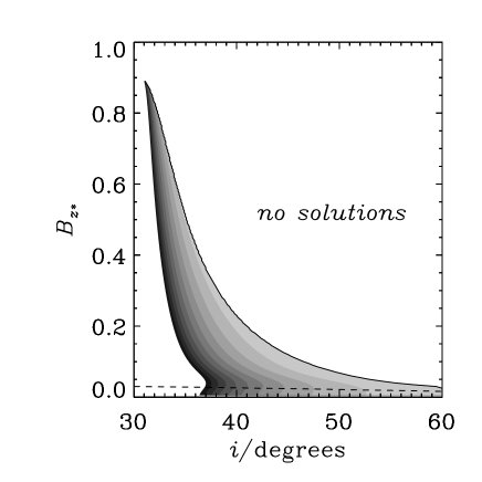
Figure 9.— Mass loss rate under the marginal stability hypothesis. Contours of $\log_{10}(\dot{m}_{\rm w}/\Sigma\Omega)$ are plotted, from $-14$ (darkest) to $-4$ (lightest). The solutions continue to smaller values of $i$, but do not extend to the right of the solid line. Below the dashed line, the atmosphere is not magnetically dominated ($\beta>1$ at the photosphere) and the outflow solution should not be trusted.

Figure 10.— Ratio of the mass loss rate to the accretion rate as a function of the strength of the magnetic field for equilibria with $i=35^{\circ}$, under the marginal stability hypothesis. The same solutions appear in Fig. 9.