Deprojecting Sunyaev-Zel’dovich statistics

Abstract

We apply the hierarchical clustering model and non-linear perturbation theory to the cosmological density and temperature fields. This allows us to calculate the intergalactic gas pressure power spectrum, SZ anisotropy power spectrum, skewness and related statistics. Then we show the effect of the non-gravitational heating. Our model confirms recent simulations yielding mass weighted gas temperature $\bar{T}_{g}\sim 0.35$ keV and reproduces the power spectra found in these simulations.

While the SZ effect contains only angular information, we show that it is possible to extract the full time resolved gas pressure power spectrum when combined with galaxy photometric redshift surveys by using a variation on the cross-correlation. This method further allows the disentanglement of the gravitational and the non-gravitational heating.

1 Introduction

One of the open questions in cosmology today is the state of the intergalactic medium (IGM). In the present popular cosmological models, a putative cosmological constant accounts for perhaps 2/3 of the energy density of the universe, and a similarly mysterious cold dark matter component accounts for 2/3 of the remainder. Of order 10% of the energy density is supposed to be accounted for by baryons (Lange et al., 2000; Tytler et al., 2000) as obtained from primordial nucleosynthesis calculation. Surprisingly, the vast majority of the baryons in the local universe is as of yet undetected. The directly observed known components consisting of stars, as well as hot and cold gas in galaxies, groups and clusters, only account for a few percent of this baryon budget (Fukugita et al., 1997). Cluster of galaxies are known to possess a large gas fraction, of order $20\%h_{50}^{-3/2}$ (Pen, 1997). This gas fraction, if representative of the universe at large, is sufficient to account for the majority of baryons in the universe (White et al., 1993). Since gravity acts on all particles equally, one expects this ratio within the virial radius of clusters to be representative of the universal fraction. In the standard bottom-up picture of structure formation, clusters are the most massive objects in the universe, and therefore the latest to form. This suggests that the majority of baryons is in a diffuse intergalactic form, which forms the intracluster medium when clusters collapse. If the baryons were in other forms, for example compact objects which formed early in the universe, it would be extremely difficult to understand how those baryons would be released back into diffuse form when clusters form.

Pen (1999) showed that the IGM must have been heated by sources other than the gravitational energy of collapse and its resulting shock waves. Its direct detection would be of significant interest to quantitatively understand the distribution and state of the IGM, and thereby infer its thermal history. Unfortunately, hot diffuse gas is difficult to detect in emission. Luckily, the Cosmic Microwave Background (CMB) scatters off all free electrons through inverse compton scattering, allowing us to “see” the IGM through scattering, in analogy to absorption. This is known as the Sunyaev-Zel’dovich effect (Zel’dovich and Sunyaev, 1969), which is becoming routinely observable. It becomes the dominant source of CMB fluctuations on arc-minute scales. Several experiments to conduct deep blank field or all sky search are under development. The upcoming CMB experiments such as AMIBA (Array for Microwave Background Anisotropy (2003)), South Pole Submillimeter Telescope (2003), Planck (2007), etc. and the current CBI (Cosmic Background Imager (2000)) are capable of detecting this angular scale. Using multi-frequency information, the SZ fluctuation can be disentangled from the primary anisotropies at all angular scales (Cooray et al., 2000a).

On the theory part, various approaches have been explored to compute the SZ angular power spectrum. Amongst these, the Press-Schechter formalism is perhaps the most widely used due to its versatility and ease of implementation (Cole and Kaiser, 1988; Makino and Suto, 1993; Artio-Barandela and Mucket, 1999; Komatsu and Kitayama, 1999; Cooray, 2000b). The authors above adopted the cluster gas model, while Da Silva et al. (1999); Refregier et al. (1999); Seljak et al. (2000) used simulations and Cooray et al. (2000a) used a simplified gas pressure bias model motivated from simulations to probe the statistics of the SZ effect.

One of the shortcomings of the SZ effect is its lack of redshift information. Since scattering is independent of redshift, the SZ effect on one hand allows a direct probe of the IGM to high redshift, on the other hand makes it challenging to disentangle the contributions arising from different redshifts. In this paper, we apply the hierarchical clustering model and non-linear perturbation theory to directly compute the SZ effect. This analytical method enables us to to extract distance information of intergalactic gas from the cross correlation of the SZ effect with galaxy surveys and at the same time, check the results of both simulations and the Press-Schechter formalism. In section 2, we develop our gas pressure model and in section 3 the SZ statistics including power spectrum and bispectrum. Section 4 contains our results on the SZ-galaxy cross correlation and the method to extract the redshift distribution of the SZ effect. The effect of non-gravitational heating and the method to extract it from overall gas pressure power spectrum are discussed in section 5. We discuss the potential inaccuracies arising from the approximations in section 6. The paper concludes with section 7.

2 Gas pressure power spectrum

The temperature distortion caused by the SZ effect (Zel’dovich and Sunyaev, 1969) is:

$$\Theta(\hat{n})\equiv\frac{\Delta T_{CMB}(\hat{n})}{T_{CMB}}=-y(\hat{n})\frac{xe^{x}}{e^{x}-1}\left[4-x/\tanh(x/2)\right]\equiv-2yS(x)$$ (1)

where $\hat{n}$ is the direction on the sky, $x=h\nu/(kT_{CMB})$, and the scattering function $S(x)\rightarrow 1$ when $x\ll 1$ (Rayleigh-Jeans tail). In this limit the SZ effect results in an apparent cooling of the CMB background. The “$y$” parameter is defined as

$$y(\hat{n})=\frac{\sigma_{T}}{m_{e}c^{2}}\int_{0}^{l(z_{cmb})}n_{e}kT_{g}dl=\frac{\sigma_{T}}{m_{e}c^{2}}\int P_{e}(\hat{n})dl=\frac{\sigma_{T}}{m_{e}c^{2}}\int\bar{P_{e}}y_{p}(\hat{n})dl$$ (2)

Here, $T_{g}$ and $n_{e}$ are the temperature and number density of free electrons, respectively. $P_{e}$ is the gas pressure. $y_{p}=P_{e}/\bar{P_{e}}=(1+\delta_{g})T_{g}/\bar{T_{g}}$ and $\bar{T_{g}}\equiv\langle(1+\delta_{g})T_{g}\rangle$ is the gas density weighted mean temperature. $dl=a(z)C(x)dx$ is the proper distance, $a(z)$ is the scale factor, $x(z)$ is the comoving distance,

$$C(x)=\frac{1}{\left[1-K(x/R_{0})^{2}\right]^{1/2}}$$ (3)

describes the geometric effect of the curved universe, $K=-1,0,1$ for open, flat and closed universes respectively, and $R_{0}=\frac{c}{H_{0}}(1-\Omega_{0})^{-1/2}$ is the curvature radius. $\rho_{0}=\rho_{c}\Omega_{0}$ is the present cosmological matter density.

Pen (1999) showed that the intergalactic medium has most likely been preheated by non-gravitational sources to $\sim 1$ keV per nucleon in order to be consistent with the observed upper bounds from the X-ray background. We adopt the model of (Pen, 1999) to express the gas distribution as a convolution of the matter distribution:

$$\delta_{g}(x)=\int\delta(x^{\prime})W_{g}(|x-x^{\prime}|)d^{3}x^{\prime}$$ (4)

This equation expresses gas as being less clumped than dark matter, partly due to the required preheating. The effective radius in the top-hat window function, which is the gas heating radius, has the typical value $\sim 1h^{-1}$ Mpc from the X-ray background constraint (Pen, 1999). For simplicity, we adopt the Gaussian window $W_{g}(r)=\exp(-r^{2}/2r_{g}^{2})/(\sqrt{2\pi}r_{g})^{3}$ ($r_{g}\sim 1/3h^{-1}$Mpc corresponds to $1h^{-1}$ Mpc top hat window). The window function for specific heating models can be obtained from hydrodynamic simulation by comparing the gas power spectrum to the dark matter power spectrum (Ma and Pen, 2000). We also need to relate the gas temperature with the density. First, we consider the gravitational heating. We adopt the cosmic energy theorem (Peebles, 1980) for the gas temperature model, which specifies the ratio between gravitational binding energy and total kinetic energy $K$. The pressure depends on the thermalized fraction of $K$. The translational kinetic energy is thermalized from the energy released when particles shell cross. A model of the thermalized energy is thus given by the difference in energy between two particles separated by a non-linear scale in Lagrangian space, which is the distance at which they can be expected to have shell crossed. The exact procedure amounts to solving the non-linear evolution equations directly. But we can treat the effect statistically in a linear fashion. In the initial linear evolution, the gravitational potential remains constant. After virialization, the gravitational energy at a fixed location remains almost constant. In an Eulerian description, we can describe the energy of particles at a final virialized location as the energy released as a particle travels from its initial position to the final virialized location. While the initial position is not exactly known, we take a spherical average over the non-linear scale to average over all possible initial locations. We thus have

$$kT_{g}=\frac{1}{6}\frac{4m_{H}}{3+5X}(\Psi-\bar{\Psi})$$ (5)

$\Psi$ is the gravitational potential, $\bigtriangledown^{2}\Psi=-4\pi G\bar{\rho}a^{2}\delta$. $\bar{\Psi}(x)=\int\Psi(r)W_{e}(|x-r|)d^{3}r$ (hereafter call the “electron window function”) is the potential averaged over the non-linear scale $r_{e}$. We choose a Gaussian window function $W_{e}(r)$ with the the non-linear scale $r_{e}$, which for $z=0$ is $r_{e}\sim 5h^{-1}$Mpc. Hereafter we will adopt this value of $r_{e}$. $X=0.76$ is the mass fraction of the hydrogen in baryonic matter. Then, $(kT_{g})_{k}\propto\delta(k)\left[1-W_{e}(k)\right]/k^{2}\equiv\delta(k)f_{e}(k)$. Here, $W_{e}(k,z)=\exp(-k^{2}r_{e}^{2}(z)/2)$ is the Fourier transform of the electron window function. Equation (5) has some unphysical statistical properties. The spatial average of the temperature, for example, is exactly zero, and for our model using Gaussian random fields, it will be negative in half the volume. But for purposes of modeling the SZ effect, temperature is only observable when multiplied by density, and regions of positive temperature will have high density, while the negative temperature regions only contribute negligibly to the SZ effect. This model is not meant to be an exact description, but hopefully captures the statistical properties, while being simple and thus exactly solvable.

In order to estimate the accuracy of these assumptions, we first compute the gas density weighted temperature and the mean $y$ parameter. We define $\delta(x)\equiv(2\pi)^{-3}\int\delta_{k}\exp(-ik\cdot x)d^{3}k$, the power spectrum $P(k)\equiv\langle|\delta_{k}|^{2}\rangle$ and the variance $\Delta^{2}(k)\equiv k^{3}P(k)/2\pi^{2}$. We adopt the initial power spectrum (Peebles, 1983; Davis et al., 1985) $P_{linear}(k)\propto k^{1+\alpha}/(1+1.7k+9k^{1.5}+k^{2})$ (here, $k$ is in unit of $\Omega_{0}h^{2}$/Mpc and we choose the Harrison-Zel’dovich-Peebles scale invariant spectrum $n=-1$ corresponding to $\alpha=0$), cluster-normalized density fluctuation at $8h^{-1}$Mpc by $\sigma_{8}=0.53\Omega^{-\beta}$ [$\beta=0.53$ for $\Lambda$CDM and $\beta=0.45$ for OCDM ] (Pen, 1998) and the Peacock and Dodds (1996) fitting formula to convert the linear $P_{linear}$ to the nonlinear $P(k)$. Then

$$\bar{T_{g}}=\langle(1+\delta_{g})T_{g}\rangle=4\pi G\rho_{0}\frac{1}{6}\frac{4m_{H}}{3+5X}(1+z)\int_{0}^{\infty}\Delta^{2}(k)W_{g}(k)f_{e}(k)\frac{dk}{k}$$ (6)

$$\bar{y}=\frac{\sigma_{T}}{m_{e}c^{2}}\int\bar{P_{e}}dl=\frac{\sigma_{T}}{m_{e}c^{2}}f_{g}\frac{\rho_{B}(0)}{2m_{H}/(1+X)}\int_{0}^{x(z_{cmb})}\bar{T_{g}}(z)(1+z)^{2}C(x)dx$$ (7)

$W_{g}(k)$ is the Fourier transform of the gas window function in equation (4), $\rho_{B}=\rho_{c}\Omega_{B}$ is the present baryonic matter density and $f_{g}$ is the mass fraction of baryonic matter in gaseous form. Since cluster gas fractions (Danos and Pen, 1998) are comparable to the baryon fraction obtained from big bang nucleosynthesis, we expect that $f_{g}\sim 1$. We use $f_{g}=0.9$, $\Omega_{B}h^{2}=0.02$ and the dimensionless Hubble constant $h=0.67$. The results for SCDM, OCDM and $\Lambda$CDM are shown in table 1 and figure 1.

In the absence of non-gravitational heating effects, we find the present $\bar{T_{g}}$ is around $0.35$ keV and the mean SZ temperature distortion $\bar{\Theta}\sim 5\times 10^{-6}$K . They are all consistent with the simulations and Press-Schechter formalism results (Refregier et al., 1999; Seljak et al., 2000).

Cosmologies	SCDM		OCDM		$\Lambda$CDM
$\Omega_{0}$	1		0.37		0.37
$\sigma_{8}$	0.53		0.83		0.90
$r_{g}/(h^{-1}$Mpc)	$1/3$	$1/6$	$1/3$	$1/6$	$1/3$	$1/6$
$\bar{T_{g}}(z=0)$/keV	0.3	0.35	0.30	0.35	0.33	0.38
$\bar{y}\times 10^{6}$	1.4	1.7	2.9	3.5	2.3	2.6

Table 1: Present day mass weighted average gas temperature $\bar{T_{g}}(z=0)$, $\bar{y}$, and temperature distortion skewness parameter $\Theta_{3}\equiv\frac{\langle(\Theta-\bar{\Theta})^{3}\rangle}{\langle(\Theta-\bar{\Theta})^{2}\rangle^{2}}$ for various cosmologies. Two different gas-mass relations are used ($r_{g}=1/3,1/6$), which only has a small effect on the results.

We define the pressure correlation function $\xi_{p}(r)\equiv\langle y_{p}(x)y_{p}(x+r)\rangle\equiv\langle[1+\delta_{g}(x)]T(x)[1+\delta_{g}(x+r)]T(x+r)\rangle/\bar{T_{g}}^{2}$. Then the pressure power spectrum

$$P_{p}(k,z) = \left[\int\Delta^{2}(k,z)W_{g}(k)f_{e}(k,z)\frac{dk}{k}\right]^{-2}\times$$

$$\left(\frac{1}{(2\pi)^{6}}\int B_{4}({\bf k_{1}},{\bf k_{2}},{\bf k_{3}},{\bf k_{4}};z)W_{g}(k_{1})f_{e}(k_{2},z)W_{g}(k_{3})f_{e}(k_{4},z)d^{3}k_{2}d^{3}k_{4}\right.$$

$$+\frac{1}{(2\pi)^{3}}\int W_{g}(k_{1})P(k_{1},z)f_{e}(k_{2},z)P(k_{2},z)\left[W_{g}(k_{1})f_{e}(k_{2},z)+W_{g}(k_{2})f_{e}(k_{1},z)\right]d^{3}k_{2}$$

$$+2\frac{1}{(2\pi)^{3}}\int B_{3}(k_{1},k_{2},k;z)W_{g}(k_{1})f_{e}(k_{2},z)f_{e}(k,z)d^{3}k_{2}$$

$$+P(k,z)f_{e}^{2}(k,z)\ )$$

Statistical isotropy implies, $\bf{k_{1}}+\bf{k_{2}}=-k_{3}-k_{4}=k$. The first term in the parentheses is from the non-Gaussian (connected) part of the four-point correlation $\langle\delta_{g}(x)T(x)\delta_{g}(x+r)T(x+r)\rangle$. $B_{4}$ is the density polyspectrum. The second term is from the Gaussian part of $\langle\delta_{g}(x)T(x)\delta_{g}(x+r)T(x+r)\rangle$. This part also produces a term $(2\pi)^{3}\delta_{D}(\bf k)$ in $P_{p}(k)$, which only affects the spatially averaged quantities such as $\langle P_{e}^{2}\rangle$ and will be included explicitly only when it is observable. The third term is from the three-point correlation $\langle\delta_{g}(x)T(x)T(x+r)\rangle+\rm permutation$. $B_{3}$ is the density bispectrum. The last term is from the raw temperature correlation $\langle T(x)T(x+r)\rangle$.

We adopt the hierarchical model (Fry, 1984) which allows all higher order correlations to be expressed as the sum of products of two point correlations over all configurations, so

$$B_{N}({\bf k_{1},...,k_{N}})=\sum_{a=1}^{t_{N}}Q_{N,a}\sum_{{\rm labelings}}\prod_{{\rm edges}}^{N-1}P_{AB}$$ (9)

$P_{AB}$ is the two point power spectrum. $a$ denotes different configurations. Coefficients $Q_{N,a}$ generally depend on configurations. In the highly non-linear regime, they degenerate (Scoccimarro and Frieman, 1999). Because the SZ effect is mostly contributed by the highly nonlinear regime, we adopt the saturated $Q_{AB}$ in the highly non-linear regime: $Q_{4}^{sat}=\frac{27(1-2^{n-1})+3^{n}+\frac{1}{2}\times 6^{n}}{1+6\times 2^{n}+3^{n+1}+6^{n+1}}$ and $Q_{3}^{sat}=\frac{4-2^{n}}{1+2^{n+1}}$ from HEPT (the Hyper-Extended Perturbation Theory) (Scoccimarro and Frieman, 1999). Here, $n$ is the linear power spectrum index and we choose the value of $n$ at $k=\sum_{i=1}^{N}(k_{i}/N)$. In this framework,

$$B_{3}(k_{1},k_{2},k_{3}) = Q_{3}(P_{1}P_{2}+P_{2}P_{3}+P_{3}P_{1})$$

$$B_{4}(k_{1},k_{2},k_{3},k_{4}) = Q_{4}\left[P_{1}P_{2}P_{3}+(3{\rm\ Permutations})+P_{1}P_{12}P_{4}+(11{\rm\ permutations})\right]$$ (10)

where $P_{i}=P(k_{i})$ and $P_{ij}=P({\bf|k_{i}+k_{j}|})$.

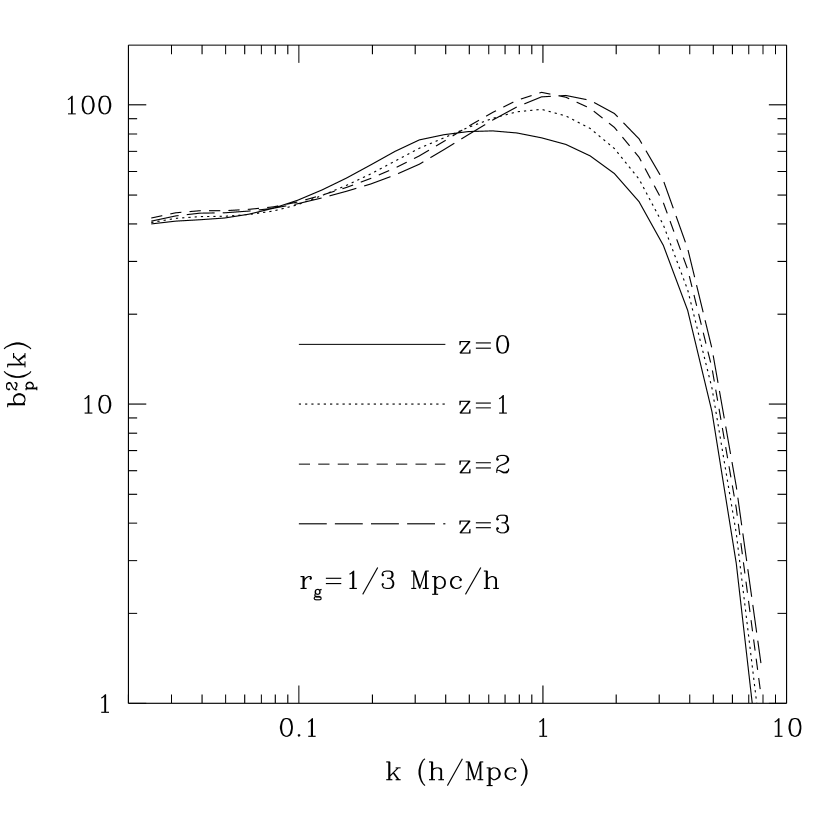
Figure 2: Gas pressure bias in $\Lambda$CDM model. Results for OCDM and SCDM are similiar.

Results are shown in figures 2 and 3. Calculations show that the non-Gaussian term is dominant in the spectrum even when $k$ is small and this non-Gaussian term itself is mostly contributed by the nonlinear regime. Besides the reason that the electron window function sweeps off most contribution from the linear regime, these behaviors reflect the strong correlation between $\delta$ and $T$ and the domination of the highly nonlinear (non-Gaussian) regime. This argues that the isotropic simplification for $Q_{N}$ is at least self-consistent. We define the gas pressure bias $b_{p}$ as $b_{p}^{2}(k,z)\equiv P_{p}(k,z)/P(k,z)$. The amplitude of $b_{p}$ varies only weakly with time. This is an expected consequence of the hierarchical model, argued as followed. The time dependence through the density power spectrum is basically canceled because Eq. (2) shows that the dependence of $P_{p}(k,z)$ over time is roughly $P_{p}(z)\propto B_{4}(z)/P^{2}(z)$. The hierarchical model implies that roughly $B_{4}(z)\propto P^{3}(z)$. Then $b^{2}_{p}(z)\equiv P_{p}(z)/P(z)\propto P^{0}(z)$. The only remaining time dependence arises from the evolution of the electron window function. Its effect is to eliminate the contribution from scales larger than several $r_{e}$. Since $r_{e}$ decreases with redshift, its evolution moves the peak of the bias to smaller scales, which should have higher bias. The bias approaches a constant ($\sim 6$ for all three cosmological models) at large scale, but it drops quickly at very small scale (due to the gas window function). This result is consistent with Refregier et al. (1999). One point worthy of mention is that, the behavior that $b_{p}$ approach a constant at large scale does not validate the constant bias model, which always produces a unit pressure-density cross correlation coefficient. But as we will see in Sec. 4, this is not the case. The pressure fluctuation variance peaks roughly at the scale of cluster core radii ($\sim 0.13h^{-1}$ Mpc), which is the direct result of the gas window function ($r_{g}\sim 1/3h^{-1}$ Mpc).

3 Statistics of Sunyaev-Zel’dovich effect on CMB anisotropies

The SZ effect on CMB anisotropies is fully described by the $n$-point correlation functions between temperature distortion $\Theta$ in different sky directions. The CMB anisotropy is decomposed into the harmonic components by:

$$\Theta(\hat{q})\equiv\frac{\delta T}{T}(\hat{q})=\sum^{l,m}a_{lm}Y_{lm}(\hat{q})$$ (11)

The CMB power spectrum is defined as $C_{l}\equiv\langle\sum_{m=-l}^{l}a_{lm}a_{lm}^{*}\rangle/(2l+1)$. The bispectrum is defined as $B_{l_{1}l_{2}l_{2}}^{m_{1}m_{2}m_{3}}\equiv\langle a_{l_{1}}^{m_{1}}a_{l_{2}}^{m_{2}}a_{l_{3}}^{m_{3}}\rangle$. They have been discussed by many authors as mentioned in the introduction section. Our model successfully reproduces these results. In contrast to the Press-Schechter models, our model relies only on direct statistical correlators that have been proposed semi-analytically with only a few free dimensionless parameter, the $Q$ saturation values, that have been verified in simulations. In the Press-Schechter model, the shape of the correlation function depends directly on the assumed structure of halos, which is a free function of the model and empirically measured in simulations. The radially averaged structure of halos, however, is not necessarily a direct predictor of correlations, unless one assumes halos to have no substructure. It is reassuring to see that our approach, which originates from the diametrically opposite theoretical bases from Press-Schechter formalism, produces consistent results and agrees with simulations.

3.1 SZ power spectrum

Since we are interested in small angular scale where the line-of-sight CMB survey depth is much larger than any correlation length, we adopt Limber’s equation (Peacock, 1999). In the Rayleigh-Jeans region we get the SZ power spectrum:

$$C_{l}=\frac{64\pi^{2}}{(2l+1)^{3}}\int_{0}^{x(z_{cmb})}\Delta^{2}_{SZ}(k,z)|_{k=l/x}C(x)x(z)dx(z)$$ (12)

where

$$\Delta_{SZ}^{2}(k,z)\equiv\left(\frac{\bar{P}_{e}(z)\sigma_{T}}{m_{e}c^{2}(1+z)}\right)^{2}\frac{1}{2\pi^{2}}k^{3}P_{p}(k,z)$$ (13)

The results are shown in figure 4 and 5. We find that (1) The SZ effect exceeds the primary CMB anisotropy at $l\sim 2000$. (2) The $C_{l}$ of SCDM is much smaller than that of OCDM and $\Lambda$CDM. This is due to the smaller $\sigma_{8}$ and faster drop of the gas temperature in SCDM with increasing redshift. (3) Because $P(k)\propto\sigma_{8}^{2--3}$ ($2$ in linear regime and $3$ in stable clustering regime) and $P_{p}(k)\propto B_{4}\propto P^{3}(k)$, we at once find that $C_{l}\propto\sigma_{8}^{6--9}$. (4) The peak contribution to $C_{l}$ depends on the angular scale, varying from $z\sim 0.4$ at $l\sim 1000$ to $z\sim 1.5$ for $l\sim 10000$. Smaller angles probe the more distant universe. These results are consistent with existing simulations and Press-Schechter formalism results.

3.2 SZ bispectrum

The SZ bispectrum is the projection of the pressure bispectrum $B^{p}_{3}(k_{1},k_{2},k_{3})$ defined by

$$\langle y_{p}({\bf k_{1}})y_{p}({\bf k_{2}})y_{p}({\bf k_{3}})\rangle\equiv B^{p}_{3}({\bf k_{1},k_{2},k_{3}})\delta_{D}({\bf k_{1}+k_{2}+k_{3}})$$ (14)

Since $y_{p}\propto\delta^{2}$, $B^{p}_{3}$ is related to 6-point density correlation function and in principle can be computed using our model. But due to the complexity of the 6-point hierarchy and the absence of extensive numerical tests, we adopt the approach of Cooray et al. (2000a) and assume a simple pressure bias model where $\delta_{p}(k,z)=b_{p}(k,z)\delta_{k}(z)$ with $b_{p}^{2}(k,z)\equiv P_{p}(k,z)/P(k,z)$. The pressure bias model states that the pressure is a linear convolution over the density. We note that this model builds in certain assumptions, which are invalid for treating cross-correlation issues address in section 4. It presumably provides a quick order of magnitude estimator, but fails on qualitative issues like galaxy-SZ cross-correlation coefficients.

In the bias model the pressure bispectrum is given as

$$B_{3}^{p}({\bf k_{1},k_{2},k_{3}};z)=\prod^{3}b_{p}(k_{i},z)B_{3}({\bf k_{1},k_{2},k_{3}};z).$$ (15)

The SZ skewness parameter,

$$\Theta_{3}\equiv\frac{\langle(\Theta-\bar{\Theta})^{3}\rangle}{\langle(\Theta-\bar{\Theta})^{2}\rangle^{2}}$$ (16)

is the easiest observable projection of the SZ bispectrum, so we show its computation as an example.

Instead of working in multipole space, we derive following equations adopting the same approximation as Limber’s equation:

$$\langle\Theta(\hat{n})^{2}\rangle=\bar{\Theta}^{2}+\frac{4}{2\pi}\int\left(\frac{\sigma_{T}\bar{P_{e}}(z)}{m_{e}c^{2}(1+z)}\right)^{2}C(x)dx(z)\times\left[\int b_{p}^{2}(k,z)P(k,z)kdk\right]$$ (17)

$$\langle\Theta(\hat{n})^{3}\rangle = \bar{\Theta}^{3}-\frac{8}{(2\pi)^{2}}\int(\frac{\sigma_{T}\bar{P_{e}}(z)}{m_{e}c^{2}(1+z)})^{3}C(x)dx(z)$$ (18)

$$\times \left[\int\prod_{i=1}^{3}b_{p}(k_{i},z)B_{3}({\bf k_{1},k_{2},k_{3}};z)k_{1}dk_{1}k_{2}dk_{2}\right]$$

where $\bf k_{3}=k_{1}+k_{2}$ and $\bf k_{1}\parallel k_{2}$. $\bar{\Theta}=-2\bar{y}\sim 5\times 10^{-6}$ is the mean temperature SZ distortion. $\bar{\Theta}^{2}$ and $\bar{\Theta}^{3}$ are from the corresponding Gaussian term in the correlation function, as explained in Eq. (2). As a reminder, $C(x)$ is the geometric function defined in Eq. (3). Though the unsmoothed $\Theta_{3}$ is not directly observable due to the absence of the window function, from the theory viewpoint, it represents the raw non-gaussianity properties. Our calculations find that $\Theta_{3}\sim 10^{6}$ (Table 1). We defined the skewness parameter (16) as the ratio of differential measurements, which might result from interferometers in the Raleigh-Jeans regime. For comparison, Cooray et al. (2000a) and Cooray (2000b) considered the absolute temperature distortion and defined the skewness parameter as $\langle\Theta^{3}\rangle/\langle\Theta^{2}\rangle^{2}$. With multi-frequency information the absolute $y$ could be measured at each point in space, and that definition of skewness could in principle be observed. The results are not too different: In our model, $\langle\Theta^{3}\rangle/\langle\Theta^{2}\rangle^{2}\sim 10^{5}$, which is similar to the result of (Cooray, 2000b) with the maximum virialized mass $\sim 10^{15}M_{\odot}$. Further work considering window function filtering and the general calculation of the SZ bispectrum can be done following the method of Cooray et al. (2000a).

4 Extracting redshift information from SZ-galaxy cross correlation

In the SZ effect, the redshift distribution of intergalactic gas is lost. Taking advantage of the cross correlations with other surveys having redshift information, we may be able to statistically extract IGM 3-D correlations and evolution. Because the SZ effect is mostly contributed by nonlinear structures at $z\sim 0.5-2$, it should have a strong cross correlation with galaxies at that redshift range. The general idea is to use a galaxy survey with coarse redshift information, where the distance information only needs enough accuracy to resolve the time evolution of the correlation function, for example $\Delta z\sim 0.2$, which can be reached by photometric redshift surveys. One then correlates each redshift bin with the SZ map, and obtains the relative contribution of that SZ slice to the total projected map.

Several questions that pose themselves in this procedure are: How big a survey area and depth does one need? What fraction of the total SZ fluctuations can be accounted using cross-correlations? Are there optimal procedures of cross-correlating? Since SZ fluctuations are a non-linear function of the galaxy field, what fraction of the signal will ever be accounted for by this approach? Do we expect the SZ-galaxy cross-correlation coefficient to depend on redshift? How big an uncertainty might arise from a time and scale dependent galaxy bias? In this section we will address each of these questions using our model, and obtain quantitative estimates.

We assume a linear bias model for the galaxy number overdensity $\delta_{G}=b\delta$. The bias $b$ is taken to be a constant for simplicity. Then, the projected galaxies number overdensity can be expressed as

$$\frac{\Delta n}{n}(\hat{q})=\int_{0}^{x(z_{G})}\delta_{G}(x\hat{q})\phi(z)C(x)dx(z).$$ (19)

$\phi(z)$ is the selection function (which we will want to vary a posteriori using the photometric redshift information), $z_{G}$ is the redshift survey depth and $C(x)$ is the geometric function defined before. The corresponding multipole moments are:

$$C_{l}^{G}=\frac{16\pi^{2}}{(2l+1)^{3}}\int_{0}^{x(z_{G})}\Delta^{2}_{G}(k,z)|_{k=l/x}\phi^{2}(z)C(z)x(z)dx(z)$$ (20)

where $\Delta^{2}_{G}=b^{2}\Delta^{2}$. The multipole moments of SZ-galaxy cross correlation are:

$$C_{l}^{SZ,G}=\frac{2\times 16\pi^{2}}{(2l+1)^{3}}\int_{0}^{x(z_{G})}\Delta^{2}_{SZ,G}(k,z)|_{k=l/x}\phi(z)C(z)x(z)dx(z)$$ (21)

with $\Delta^{2}_{SZ,G}(k,z)=\frac{\bar{P_{e}}\sigma_{T}}{m_{e}c^{2}(1+z)}\frac{1}{2\pi^{2}}k^{3}P_{p,G}(k)$. $P_{p,G}$ is the Fourier transform of $\langle y_{p}({\bf x})\delta_{G}({\bf x+r})\rangle$.

$$P_{p,G}(k,z)=b\times\frac{P(k)f_{e}(k)+\frac{1}{(2\pi)^{3}}\int B_{3}(k_{1},k_{2},k)W_{g}(k_{1})f_{e}(k_{2})d^{3}k_{2}}{\int\Delta^{2}(k)W_{g}(k)f_{e}(k)\frac{dk}{k}}$$ (22)

We have used $\bf k=k_{1}+k_{2}$. It is useful to define the cross correlation coefficient

$$r(k,z)\equiv\frac{\Delta^{2}_{SZ,G}(k,z)}{\Delta_{SZ}(k,z)\Delta_{G}(k,z)}\equiv\frac{P_{p,G}(k,z)}{\sqrt{P_{p}(k,z)P(k,z)}}$$ (23)

In $P_{p,G}$, the $B_{3}$ term is dominant. In $B_{4}$ there are 16 hierarchical terms and in $B_{3}$ there are three hierarchical terms. Different term dominates in different regions. Calculation shows that, roughly there are three regions: (a) $k\lesssim 0.1{\rm h/Mpc}$. 4 terms ( $P_{12}(2P_{1}P_{4}+P_{1}P_{3}+P_{2}P_{4})$ ) dominate $B_{4}$ and 2 terms ( $P_{3}P_{1}+P_{3}P_{2}$ ) dominate $B_{3}$. $r\simeq Q_{3}/Q_{4}^{1/2}\simeq 0.9$ ($n\sim-1.5$). (b) $k\lesssim 0.1{\rm h/Mpc}\lesssim 10{\rm h/Mpc}$. Each hierarchical term in $B_{3}$ and $B_{4}$ has about the same contribution to $P_{p,G}$ and $P_{p}$, respectively. $r(k,z)\sim 3/4\times Q_{3}/Q_{4}^{1/2}\sim 0.7$ ($n\sim-1.5$). This region contributes most of the SZ effect, as seen from figure 3. Unless explicitly notified, hereafter we will adopt the value of $r$ in this region. We only show the result of this region in Figure 6. (c) $k\gtrsim 10{\rm h/Mpc}$. This is the opposite case to the case (a). $r\simeq Q_{3}/\sqrt{12Q_{4}}\simeq 0.3$ ($n\sim-1.5$). No significant time dependence is found. The corresponding cross correlation coefficients in multipole space are:

$$Corr(l,\phi)=\frac{C_{SZ,G}(l,\phi)}{\left[C_{SZ}(l)C_{G}(l,\phi)\right]^{1/2}}$$ (24)

We now use the photometric redshift information from the galaxy survey to vary the selection function $\phi$. We pick the weighting which maximizes (24). This allows the measurement of one number in the SZ to yield a full function of redshift $z$. Since (24) depends on one variable $l$, we can in principle measure an optimal redshift weighting $\phi(z)$ at each $l$. The cross correlation variation has allowed us to measure a two dimensional cross-correlation function from a one dimensional observable in the SZ and a two dimensional observable in the galaxies.

The selection function to maximize $Corr(l)$ is obtained from the variation $\frac{\delta Corr(l,\phi)}{\delta\phi}=0$. We denote this selection function as $\phi_{M}(l,z)$ and find that

$$\phi_{M}(l,z)=\alpha(l)\frac{\Delta^{2}_{SZ,G}(k,z)}{\Delta^{2}_{G}(k,z)}|_{k=l/x(z)}$$ (25)

Here, $\alpha(l)$ is a constant to be determined later by the observational data. The optimized $C^{M}orr$ is:

$$C^{M}orr(l)=\left[\frac{\int_{0}^{z_{G}}\Delta^{2}_{SZ,G}\phi_{M}C(x)x(dx/dz)dz}{\int_{0}^{z_{cmb}}\Delta^{2}_{SZ}C(x)x(dx/dz)dz}\right]^{1/2}=\left[\frac{\int_{0}^{z_{G}}\frac{\Delta^{4}_{SZ,G}}{\Delta_{G}^{2}}C(x)x(dx/dz)dz}{\int_{0}^{z_{CMB}}\Delta_{SZ}^{2}C(x)x(dx/dz)dz}\right]^{1/2}$$ (26)

Results are shown in figure 7. Following the same estimation as in $r(k,z)$, $C^{M}orr(l)\simeq 3/4\times Q_{3}/Q_{4}^{1/2}\simeq 0.7$. The observed $C^{M}orr(l)$ may be smaller because of the limited galaxy survey depth.

The observationalrocedure to extract the redshift information is as follows. 1. Start with a random guess for $\phi(z)$, e.g. $\phi=1$ . 2. Given a photometric galaxy survey and SZ survey, measure $C_{SZ}(l)$, $C_{G}(l,\phi)$ and $C_{SZ,G}(l,\phi)$ from angular correlation functions $\langle\Theta(\hat{n})\Theta(\hat{n}+\hat{\theta})\rangle$, $\langle\frac{\Delta n}{n}(\hat{n})\frac{\Delta n}{n}(\hat{n}+\hat{\theta})\rangle$ and $\langle\Theta(\hat{n})\frac{\Delta n}{n}(\hat{n}+\hat{\theta})\rangle$, respectively. 3. Vary $\phi$ to maximize $Corr(l)$ for a specific $l$, therefore obtain $\phi_{M}(l,z)$. 4. Apply Eq.(25) to infer $\Delta^{2}_{SZ,G}(l/x(z),z)$, up to a constant $1/\alpha(l)$, from the directly measured $\Delta^{2}_{G}$ from the galaxy survey. Furthermore, Eq. (21) enables us to infer $\alpha(l)$ from the observed $C_{l,obs}^{SZ,G}$.

$$\alpha(l)=\left[\frac{2\times 16\pi^{2}}{(2l+1)^{3}}\int_{0}^{z_{G}}\phi_{M}^{2}(l,z)\Delta_{G}^{2}[l/x(z),z]C(z)x(z)dx/dzdz\right]/C_{l,obs}^{SZ,G}$$ (27)

5. Combine Eq.(23) and Eq.(25) to obtain the time resolved SZ power spectrum, up to a factor $r(l/x(z),z)^{-2}$.

$$\Delta^{2}_{SZ}(k,z)=\phi_{M}^{2}(l,z)\Delta^{2}_{G}(l/x(z),z)/[r^{2}(l/x,z)\alpha^{2}(l)]$$ (28)

In our model $r(l/x(z),z)$ is almost a constant $\simeq 1/0.7^{2}\simeq 2$ independent of cosmological models or redshifts (see Figure 6). This gives a theoretical estimate of $\Delta^{2}_{SZ}(l/x,z)$. 6. $1/r^{2}$ nomalizes the observed SZ anisotropy multipole $C_{l}^{obs}$ and the SZ temperature variance. Apply Eq. (12) to integrate $\Delta^{2}_{SZ}$ obtained above with $1/r^{2}=1$ and compare with $C_{l}^{obs}$, we will obtain the averaged $1/r^{2}$.

$$\langle\frac{1}{r^{2}(l/x(z),z)}\rangle=C_{l}^{obs}/\left[\frac{64\pi^{2}}{(2l+1)^{3}}\int\phi_{M}^{2}(l,z)\Delta^{2}_{G}[l/x(z),z]/\alpha^{2}(l)C(x)x(z)dx/dzdz\right]$$ (29)

7. Follow the same steps to obtain $\Delta^{2}_{SZ,G}(l/x(z),z)$ and $\Delta^{2}_{SZ}(l/x(z),z)$ at different $l$.

Since for $C_{SZ}(l)$ at different angular scale $l$, $\langle 1/r^{2}(l/x,z)\rangle$ is determined roughly by $r(l/x(z_{p}),z_{p})$ ($z_{p}\sim 1$ is the redshift with peak contribution to $C_{l}$. See Fig. 5), we can even get some idea about the scale dependence of $r(k,z)$. Thus, the total projected SZ autocorrelation give a consistency check on the reconstructed time resolved power spectrum from the galaxy-SZ cross correlation. Furthermore, the galaxy bias and its time dependence have completely dropped out of the calculation, and are thus not expected to affect the results at all. Then, in principle, SZ-galaxy correlation plus SZ CMB anisotropy provide a consistent and powerful method to extract all time evolution information of the IGM pressure power spectrum.

Noise and cosmic variance put constraints on the feasibility of our procedure. (1) Limitation of CMB resolution degrades our method. The measured range of $k$ is $[l_{1}/x(z),l_{2}/x(z)]\sim[1_{1}/3000z,l_{2}/3000z]h$/Mpc. Here, $[l_{1},l_{2}]$ is the range of the CMB experiment. In order to detect the peak of $\Delta_{p}^{2}$ ( around $k=3h$/Mpc as shown in Fig. 3), $z\leq l_{2}/9000$. For CBI ($630\leq l\leq 3500$), we are only able to detect $z\leq 0.4$. AMIBA will measure $l\leq 28500$ and South Pole Submillimeter Telescope (2003) will measure $l\leq 40000$. They will allow us to measure the gas power spectrum up to $z\sim 3$ and $z\sim 4$, respectively. (2) Observational errors impose further constraints. Suppose that the galaxy survey covers a fraction $f_{G}$ of the sky and the $i$-th survey region (For example, if the redshift accuracy is $\Delta z$, then we can divide the galaxies into redshift bins with $0\leq z\leq\Delta z$, $\Delta z\leq z\leq 2\Delta z$, etc. ) have $N_{i}$ observed galaxies. The CMB observation covers a fraction $f_{cmb}$ of sky and the $C_{l}$ is averaged over the band $[l-\Delta l/2,l+\Delta l/2]$. Then the galaxy number count causes the Poisson error:

$$\frac{\Delta C_{G}}{C_{G}}\sim\frac{\Delta C_{SZ,G}}{C_{SZ,G}}\sim\left[f_{G}\times min(N_{i})\right]^{-1/2}$$ (30)

(3) The cosmic variance of the $C_{l}$ also cause errors. Recalling that $C_{l}=\sum a_{lm}a_{lm}^{*}/(2l+1)$ and $a_{lm}\propto\delta T\propto b_{p}\delta$, we get:

$$\frac{\Delta C_{l}}{C_{l}}=\sqrt{\frac{\langle C_{l}^{2}\rangle-\langle C_{l}\rangle^{2}}{\langle C_{l}\rangle^{2}}}\sim\sqrt{\frac{S_{4}\sigma_{R}^{2}}{(2l+1)\Delta lf_{cmb}}}\sim\sqrt{\frac{1}{10(l/2000)\Delta lf_{cmb}}}$$ (31)

Here, $\sigma^{2}_{R}$ is the density dispersion over smoothing scale $R\sim h/$Mpc. We already use the typical value of $S_{4}\sim 40$ and $\sigma^{2}_{R}(z=1)\sim 10$. The corresponding error caused in $\phi_{M}$ is:

$$\frac{\Delta\phi}{\phi_{M}}\sim\sqrt{\frac{\Delta Corr}{\phi^{2}_{M}\frac{\delta^{2}Corr}{\delta\phi^{2}}|_{\phi_{M}}}}\sim\left[(10(l/2000)\Delta lf_{cmb})^{-1}+f_{G}^{-1}\times min(N_{i})^{-1}\right]^{1/4}$$ (32)

Recalling that $\Delta^{2}_{SZ}\propto\phi_{M}^{2}$, requiring a $40\%$ accuracy on $\Delta^{2}_{SZ}$ would impose that (a) $f_{G}\times min(N_{i})\geq 10^{3}$. Each survey regions must be large enough in order to contain sufficient number of galaxies and must be small enough to ignore the evolution. We may choose redshift bands of each survey region $\Delta z_{i}\sim 0.1$. Then the number of galaxies observed $N_{O}$ has to satisfy $N_{O}\geq 10^{3}z_{G}/\Delta z_{i}/f_{G}$. For SDSS (Sloan Digital Sky Survey (2000)), which covers one quarter of the sky and probes more than one million galaxies with photometric redshift up to $z\sim 1$, the requirement $N_{O}\geq 10^{5}$ is easily satisfied. The measurement of the intergalactic gas at redshift z requires the galaxy survey at least up to that redshift (equation 25), so we need deeper galaxy survey in order to probe the gas beyond $z\sim 1$. (b) $f_{cmb}\Delta l\geq 10^{2}(2000/l)$. For CMB experiments with relatively lower resolution, larger sky coverage is required. For example, though Planck only measures $l\leq 2000$, it covers the whole sky and therefore satisfies this condition. For those with much higher resolution such as AMIBA and Submillimeter Telescope, the required sky coverage can be relaxed to the order of $1\%$.

This variation method only depends on the assumption that the cross correlation coefficient $r(k,z)$ is approximately a constant, which is the direct result of the hierarchical model and has only weak dependence on the gas model and cosmologies. Furthermore, the hierarchical model is strongly supported by the consistency of the CMB SZ power spectrum dependence on $\sigma_{8}$ and the behavior of the gas bias between our model and simulations. Since the averaged $r(k,z)$ is measurable, our method does not rely much on the theoretical value of $r(k,z)$ and thus observationally consistent.

5 Non-gravitational heating effect

Pen (1999) has shown that the IGM has most likely been preheated by non-gravitational energy sources with energy injection $E_{NG}\sim 1$ keV per nucleon. This section is devoted to consider this effect. Because the relation between the gravitational heating and the non-gravitational heating is very uncertain, we only consider two extreme cases. The first one is that the non-gravitational heating is perfectly correlated with the gravitational heating, then we can change Eq. (5) to:

$$kT_{g}=\frac{1}{6}(1+\beta)\frac{4m_{H}}{3+5X}(\Psi-\bar{\Psi})$$ (33)

We will append all former results from gravitational heating with a superscript ’A’ (Adiabatic). Here, $\beta\equiv T_{NG}/\bar{T_{g}}^{A}$ represents the ratio of the non-gravitational heating and the gravitational heating. $kT_{NG}=8/3/(3+5X)E_{NG}$. $E_{NG}\sim 1$ keV corresponds to $\beta\sim 1$. All former results are not affected by this change except $\bar{T_{g}}$, $\bar{y}\propto\bar{T_{g}}$, $C_{l}\propto\bar{T_{g}}^{2}$ and $\Theta_{3}\propto 1/\bar{T_{g}}$ due to the dependence $\bar{T_{g}}\propto(1+\beta)$. Figure 1 and 4 need to be changed correspondingly. Figure 5 and 7 will change only when $\beta$ is time-dependent. All other figures remain the same.

The second case is that non-gravitational heating is uncorrelated with local density, then, Eq. (5) changes to:

$$kT_{g}=\frac{1}{6}\frac{4m_{H}}{3+5X}(\Psi-\bar{\Psi})+kT_{NG}(z)$$ (34)

$\bar{T_{g}}=\bar{T_{g}}^{A}+T_{NG}=[1+\beta(z)]\bar{T_{g}}^{A}$. Then, the corresponding new results following the same definitions are:

$$P_{p}(k,z) = \left[P^{A}_{p}(k,z)+(2\pi)^{3}\delta_{D}({\bf k})(2\beta+\beta^{2})+2\beta P^{A}_{SZ,\delta}(k,z)+\beta^{2}P(k,z)\right]/(1+\beta)^{2}$$ (35)

$$= \frac{(b_{p}^{A})^{2}+2\beta r^{A}b_{p}^{A}+\beta^{2}}{(1+\beta)^{2}}\times P(k,z)\ ({\rm when}\ k\neq 0)$$

$$P_{p,G}(k,z)=\frac{b}{1+\beta}\times\left[P^{A}_{p,\delta}(k,z)+\beta P(k,z)\right]=b\times\frac{r^{A}b^{A}_{p}+\beta}{1+\beta}P(k,z)$$ (36)

$$b_{p}(k,z)=\frac{\sqrt{(b_{p}^{A})^{2}+2r^{A}b^{A}_{p}\beta+\beta^{2}}}{1+\beta}$$ (37)

$$r(k,z)=\frac{r^{A}b_{p}^{A}+\beta}{\sqrt{(b^{A}_{p})^{2}+2r^{A}b^{A}_{p}\beta+\beta^{2}}}$$ (38)

Here, $P_{p,\delta}^{A}=P^{A}_{p,G}/b$ is the Fourier transform of $\langle y_{p}^{A}({\bf x})\delta({\bf x+r})\rangle$. The expression of the optimal selection function $\phi_{M}$ (Eq. 25) is not affected at all. Equation (38) tells us that $r^{A}\leq r\leq 1$. As expected, when $\beta\ll b_{p}^{A}$, we reduce to our former results and when $\beta\gg b_{p}^{A}$, we obtain the bias model. There are three regions: (a) $k\gg 1/r_{g}\sim 3h$/Mpc. We always have $\beta\gg b_{p}^{A}$, $b_{p}\rightarrow\beta/(1+\beta)$ and $r\rightarrow 1$. Our redshift extraction method works well with $r\simeq 1$ in this region. Because this region is dominated by non-gravitational heating, high resolution CMB experiments are able to measure $\Delta^{2}_{SZ}$ in this region and enable us to directly obtain the information of the non-gravitational heating. Since $b_{p}$ does not approach zero as before, $\Delta^{2}_{SZ}\propto\Delta^{2}$ increases with increasing $k$. This behavior will move the peak of SZ power spectrum to larger $l$ while increasing the amplitude of SZ power spectrum. (b) $k\lesssim 6h$/Mpc. Then, $b_{p}^{A}\sim 8\gg\beta(0)\sim 1$, so $b_{p}(z)$ will decrease roughly by a factor $(1+\beta(z))$. The resulting $r$ is bigger than our former results, but it still remains roughly a constant with respective to space and time, so our redshift extraction method works well. (c) The intermediate region ( the range $b_{p}^{A}\sim\beta$, roughly $6{\rm h/Mpc}\lesssim k\lesssim 10{\rm h/Mpc}$.), $r$ varies from $\sim 0.7$ to 1. Our redshift deprojection method still works, but with a larger error. The discussion of the observational requirement is not affected at all. The new $Corr$ should differ only a little bit from the former result due to its dimentionless definition. Roughly, $C_{l}\propto(1+\beta)^{2}$, bispectrum $\propto(1+\beta)^{3}$ and skewness $\Theta_{3}\propto(1+\beta)^{-1}$.

Our knowledge on the non-gravitational heating is very limited, and presumably depends on the poorly understood physics of star formation and supernovae dynamics. It is not even known if the heating was pre or post structure formation. We have surveyed two simple but different models of non-gravitational heating to demonstrate the range of effects it may have on the correlations. The above equations show the basic procedure to include the non-gravitational heating and the possible effects. So we do not plan to constrain to a highly hypothetical model and do the calculation. For the purpose of estimation, we may either assume a step function for $T_{NG}$ ($T_{NG}(z)=T_{NG}(0)$ for $z<z_{NG}$. Otherwise, $T_{NG}=0$.) or $T_{NG}(z)=T_{NG}(0)(1+z)^{-\gamma}$. The upper limit of ’$y$’ parameter $y\leq 1.5\times 10^{-5}$ from COBE/FIRAS (Fixsen, et al., 1996) put constraints on the value of $z_{NG}$ and $\gamma$. For example, when $T_{NG}=1$ keV, $\gamma>1.5$ or $z_{NG}<3$. Further simplification can be made by taking the fitting formula of $(b^{A}_{p})^{2}$ and $r^{A}\simeq\bar{r}^{A}\simeq 0.7$. We show some examples (Figure 8,9 and 10).

When combining CMB experiments with galaxy surveys, we have four observables: $C_{l}$, $\Delta^{2}_{G}(k,z)$, $\Delta^{2}_{SZ,G}(k,z)=\phi_{M}(k,z)\Delta^{2}_{G}(k,z)$ and $\bar{r}(k)$. If $r(k,z)$ is not a strong function of time and scale, we can solve for $\Delta^{2}_{SZ}(k,z)$. If the behavior of $b_{p}(k,z)$ as discussed above is correct, we obtain the fifth observable $\beta(z)$ from the small scale behavior of $\Delta^{2}_{SZ}$.

6 Discussion

Let us now address some potential systematic shortcomings in our simplified model. (1) Our model relies on the adopted gas-dark matter density relation (Eq. 4), the (non-local) temperature-density relation (Eq. 5) and the non-gravitational heating. In case that only the gravitational heating is included, apart from intrinsic problems addressed in section 2, our model contains two free parameters: the gas-dark matter smoothing length, and the temperature-potential smoothing length. These parameters only weakly affect the pressure power spectrum and pressure bias, which are defined in terms of dimensionless functions. The normalization is expressed in terms of the mass weighted temperature, $\bar{T_{g}}$. We see in Table 1 that the gas smoothing only has a small effect. A preheating of 1 keV as proposed by Pen (1999) has a factor of order unity impact on the temperature, and about factor of 4 effect on the CMB anisotropy spectrum and 8 on the bispectrum, while the skewness will decrease by about 50%. We provide a convenient method to include such effects. Hydro simulations are able to measure the gas-DM relation and the $T-\Psi$ relation and will further improve our work. Fortunately, the main goal of our model—the extraction of the 3-D gas information is least affected, since it depends only on the cross-correlation coefficient (23) and Figure 6, which does not vary a lot even including non-gravitational heating. (2) The galaxy bias model we adopt may be too simple. In our redshift extraction method of the gas pressure power spectrum, the only bias dependency comes from $r(k,z)$. We speculate that, even for a realistic galaxy bias model, $r(k,z)$ should be close to a constant, which still enable us to extract $\Delta^{2}_{SZ}$. (3) $Q_{N}^{sat}$. The value of $Q_{N}^{sat}$ in HEPT is a function of the power index of a power law power spectrum. We have extended it to the CDM power spectrum and choose the power index at $\sum k_{i}/N$. Because SZ effect is mainly contributed by the non-linear regime with $n\sim-1.5$, HEPT is applicable and the resulting $Q_{N}$ does not vary a lot. More importantly, $Q_{3}/Q_{4}^{1/2}$ only has a weak dependence on $n$. This behavior ensures that $r(k,z)$ has least dependence on our assumptions about $Q_{N}^{sat}$.

7 Conclusions

We have presented a new tool to compute power spectra and other statistics of SZ fluctuations based on hierarchical clustering and scaling. This approach describes the two point correlation of non-linear observables, such as the SZ $y$ parameter in terms of two point correlation functions, which directly maps to the observed angular power spectrum. We have demonstrated that this approach is feasible, and produces results consistent with simulations and Press-Schechter approaches. We then addressed the problem of measuring the redshift evolution of the SZ effect through cross correlation with galaxy surveys containing coarse photometric redshift information. We have shown that a variational method allows the redshift deconvolution which does not depend on galaxy biasing. The only model dependent quantity is the cross correlation coefficient $r$ between galaxies and gas pressure, whose value has least dependence on the gas density model and the gas temperature model.

Our quantitative estimates suggest that, when combining CMB experiments either with high resolution such as AMIBA and South Pole Submillimeter Telescope or with high sky coverage such as Planck and deep broad photometric galaxy surveys such as Sloan, our method is able to extract the redshift evolution information of intergalactic gas, such as the full time resolved gas pressure power spectrum, even without requiring the knowledge of galaxy bias. It is even capable of disentangling the contribution from the gravitational heating and those from the non-gravitational heating. This method serves as a powerful probe to this primary component of cosmic baryons to high redshift. The model also provides an alternative to simulations and the Press-Schechter formalism to calculate the CMB SZ power spectrum and bispectrum. We successfully reproduce, when no non-gravitational heating presents, the mass weighted gas temperature $\bar{T_{g}}(\sim 0.35$ keV), the pressure power spectrum, the pressure bias ($\sim 8$, but scale dependent), the mean SZ temperature distortion ($\sim 5\times 10^{-6}$ K), the SZ power spectrum and the skewness parameter ($\sim 10^{6}$). With our transform formulas, non-gravitational heating is easily included and we have estimated its effects on the correlations.

Figure 1: The evolution of the gas density averaged temperature. Smaller $r_{g}$ produces higher $\bar{T_{g}}$.

Figure 3: Gas pressure variance $\Delta_{p}^{2}\equiv\frac{k^{3}}{2\pi^{2}}P_{p}(k)$. Results for OCDM and SCDM are similiar.

Figure 4: CMB anisotropy caused by SZ effect in various models. $r_{g}=1/3h^{-1}$Mpc. Smaller $r_{g}$ will move peaks to larger $l$ ( smaller angle) and larger amplitude.

Figure 5: SZ effect contribution from different redshift, defined as $\frac{\Delta^{2}_{y}(k,z)|_{k=l/x}C(x)x(z)\frac{dx}{dz}z}{\int_{0}^{z_{cmb}}\Delta^{2}_{y}(k,z)|_{k=l/x}C(x)x(z)\frac{dx}{dz}dz}$. We show a $\Lambda$CDM model ($r_{g}=\frac{1}{3}/h$ Mpc). Results for SCDM and OCDM are similiar. Smaller $r_{g}$ moves peaks to smaller $z$ and lower height.

Figure 6: SZ-Galaxy cross correlation coefficients in real space for a $\Lambda$CDM model. Results have almost no dependence on cosmological models and gas model parameters. The region shown is the most relevant region of SZ effect, as shown in figure 3. The behavior of $r(k,z)$ in other regions is estimated in Sec. 4.

Figure 7: SZ-Galaxy cross correlation coefficients in multipole space. Results have almost no dependence on cosmological models and gas model parameters.

Figure 8: $b_{p}^{2}(k,z)$ and $\Delta^{2}_{p}(k,z)$ when non-gravitation heating is considered. $kT_{NG}=0.39{\rm keV}(1+z)^{-3}$ is assumed. The time evolution of $b_{p}^{2}$ is partly due to the evolution of $\beta$.

Figure 9: $\Delta^{2}_{p}(k,z)$ when non-gravitation heating is considered. $kT_{NG}=0.39{\rm keV}(1+z)^{-3}$ is assumed. The distinctive behavior of $\Delta^{2}_{p}$ at small scales ($k\gtrsim 10\rm{h/Mpc}$) is due to the non-gravitational heating and the measurement of this region will help us to extract the non-gravitational heating information.

Figure 10: $r(k,z)$ when non-gravitational heating is considered with same assumptions as in figure 8.

.

References

- Array for Microwave Background Anisotropy (2003) AMIBA, 2003, http://www.asiaa.sinica.edu.tw/Research/AMIBA/amiba.html
- Artio-Barandela and Mucket (1999) Atrio-Barandela, F. and Mucket, J., 1999, ApJ, 515, 465
- Bernardeau (1994) Bernardeau, F., 1994, A&A, 291, 697
- Cole and Kaiser (1988) Cole, S. and Kaiser, N., 1988, MNRAS, 233, 637
- Cooray et al. (2000a) Cooray, A., Hu, W. and Tegmark, M., 2000a, submitted to ApJ, astro-ph/0002238
- Cooray (2000b) Cooray, A., 2000b, submitted to PRD, astro-ph/0005287
- Cosmic Background Imager (2000) CBI, http://astro.caltech.edu/$^{∼}$tjp/CBI/
- Danos and Pen (1998) Danos, R. and Pen, U.L., 1998, astro-ph/9803058
- Davis et al. (1985) Davis, M., et al. 1985, ApJ, 292, 371
- Da Silva et al. (1999) Da Silva, A.C., et al., 1999, submitted to MNRAS, astro-ph/9907224
- Fixsen, et al. (1996) Fixsen, D.J., et al., 1996, ApJ, 473, 576
- Fry (1984) Fry, J.N., 1984, ApJ, 279, 499
- Fukugita et al. (1997) Fukugita, M., Hogan, C.J. and Peebles, P.J.E, astro-ph/9712020
- Lange et al. (2000) Lange, A.E. et al. 2000, astro-ph/0005004
- Komatsu and Kitayama (1999) Komatsu, E. and Kitayama, T., 1999, ApJ, 526, L1
- Ma and pen (2000) Ma, C.P. and Pen, U.L., in preparation, 2000
- Makino and Suto (1993) Makino, N., and Suto, Y., 1993, ApJ, 405, 1
- Matsubara (1999) Matsubara, T., 1999, ApJ, 525, 543
- Peacock and Dodds (1996) Peacock, J.A. and Dodds, S.J. 1996, MNRAS, 280, L19
- Peacock (1999) Peacock, J., Cosmological Physics, Cambridge University Press, 1999
- Peebles (1980) Peebles, P.J.E., The Large-Scale Structure of The Universe, 1980, Princeton University Press
- Peebles (1983) Peebles, P.J.E., 1983, ApJ, 263, L1
- Pen (1997) Pen, U.L., 1997, New Astronomy, 2, 309
- Pen (1998) Pen, U.L., 1998, ApJ, 498, 60
- Pen (1999) Pen, U.L., 1999, ApJ, 510, L1
- Planck (2007) Planck, 2007, http://astro.estec.esa.nl/SA-general/Projects/Planck/
- Refregier et al. (1999) Refregier, A., Komastu, E., Spergel, D.N. and Pen, U.L., 1999, submitted to PRD, astro-ph/9912180
- Scoccimarro and Frieman (1999) Scoccimarro, R. and Frieman, J., 1999, ApJ, 520, 35
- Seljak et al. (2000) Seljak, U., Burwell, J. and Pen, U.L., 2000, submitted to PRD, astro-ph/001120
- South Pole Submillimeter Telescope (2003) Submillimeter Telescope, http://cfa-www.harvard.edu/$^{∼}$aas/tenmeter
- Tytler et al. (2000) Tytler, D., O’Meara, J.M., Suzuki, N. and Lubin, D. 2000, astro-ph/0001318
- Sloan Digital Sky Survey (2000) Sloan Digital Sky Survey, http://www.sdss.org
- White et al. (1993) White, S.D.M., Navarro, J.F., Evrard, A.E., Frenk, C.S. 1993, Nature, 366, 429
- Zel’dovich and Sunyaev (1969) Zel’dovich, Y.B. and Sunyaev, R., 1969, Ap&SS, 4, 301
.