Abstract

Minkowski functionals constitute a family of order parameters which discriminate spatial patterns according to size, shape and connectivity. Here we point out, that these scalar descriptors can be complemented by vector–valued curvature measures also known as Quermaß vectors. Using examples of galaxy clusters, we demonstrate that the Quermaß vectors provide additional morphological information on directional features and symmetries displayed by spatial data.

Physica A

PACS: 02.40.Ft (conv. sets and geometrical inequalities), 02.40.Vh (global analysis and analysis of manifolds), 98.65.Cw (clusters of galaxies)

Key words: methods: morphology, integral geometry, cluster substructure, large–scale structure

1 Introduction

Spatial patterns originating from the polymorphic aggregation of matter in Nature occur on vastly different length–scales and with unlimited variety. The pattern shown in Figure 1 displays an isodensity contour of the smoothed galaxy distribution in our Universe, but it could also represent a biological structure obtained with X–ray tomography, for instance.
The visual impression of such patterns may already convey valuable insights on the formation processes or the functionality of those structures. However, for unbiased inferences as well as for comparison with model simulations, for example, one needs objective and quantitative measures to characterize the geometry and topology of typical structural motifs.

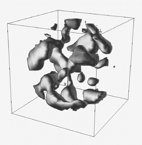
Figure 1: An isodensity contour of the galaxy distribution within the PSCz survey (from the PSCz homepage at http://star-www.dur.ac.uk/cosmology/theory/pscz.html).

In the present paper we discuss a family of suitable measures, which include, besides the scalar Minkowski functionals, their vectorial relatives – the curvature centroids, or Quermaß vectors. Taken together, these measures constitute a complete class of morphometric order–parameters for spatial patterns formed – or approximated – by the set union and intersection of an arbitrary but finite number of convex “pixels” or “voxels”.
The usefulness of Minkowski functionals has already been demonstrated by the analysis of galaxy catalogues and simulations of large–scale structure [11, 10, 16, 18], as well as of the temperature distribution in maps of the microwave background radiation [19]. Furthermore, they were used to characterize the morphology of spinodal decomposition [15] and of patterns arising within reaction–diffusion systems [13]. Here, we focus attention on the less familiar Quermaß vectors and illustrate their versatility with the examples of galaxy clusters and with patterns generated by lattice automata.

2 Morphometric order parameters

In this section we recall the definitions of Minkowski functionals and Quermaß vectors. The presentation will be brief and informal. Readers, who are interested in mathematical details, may consult refs. [9, 20, 21, 8, 14].
Consider a compact convex point set (body) $K\subset{\mathbb{E}}^{d}$, in Euclidean d–dimensional space with volume

$$V_{0}(K)=\int_{K}{\rm d}^{d}{\mathbf{x}}>0$$ (1)

and with center of mass at the position:

$${\mathbf{p}}_{0}\equiv{\mathbf{V}}_{0}/V_{0}\quad,\quad{\mathbf{V}}_{0}(K)=\int_{K}{\mathbf{x}}{\rm d}^{d}{\mathbf{x}}\;\;\;.$$ (2)

Now, we let the body grow to form a parallel body $K_{\epsilon}$, $\epsilon>0$, by including all points ${\mathbf{x}}$ within a distance $d(K,{\mathbf{x}})\leq\epsilon$ to $K$. From Steiner’s theorem [12] we know that the volume $V_{0}(K_{\epsilon})$ of $K_{\epsilon}$ is a finite polynomial in $\epsilon$,

$$V_{0}(K_{\epsilon})=\sum_{i=0}^{d}\binom{d}{i}\omega_{i}V_{i}(K)\epsilon^{i}\;\;\;,$$ (3)

where $\omega_{i}=\pi^{i/2}/\Gamma(1+i/2)$ denotes the volume of the $i$–dimensional unit ball. The coefficients $V_{i}(K)$ define the Minkowski functionals of the body $K$. Since the volume $V_{0}(K_{\epsilon})$ depends on the shape of $K$, the functionals $V_{i}(K)$ contain morphological information on the original body.
A corresponding expansion holds for the vectorial ${\mathbf{V}}_{0}(K)$ [9],

$${\mathbf{V}}_{0}(K_{\epsilon})=\sum_{i=0}^{d}\binom{d}{i}\omega_{i}{\mathbf{V}}_{i}(K)\epsilon^{i}\;\;\;,$$ (4)

which defines the Quermaß vectors ${\mathbf{V}}_{i}(K),\;0\leq i\leq d$. Under translations (t) and rotations (r) of the body $K$, the Minkowski functionals are motion–invariant scalars, whereas the Quermaß vectors are motion–equivariant:

$${\mathbf{V}}_{i}(tK)= {\mathbf{V}}_{i}(K)+{\mathbf{t}}V_{i}(K),$$ (5a)

$${\mathbf{V}}_{i}(rK)= R(r){\mathbf{V}}_{i}(K),$$ (5b)

where $R(r)$ denotes an orthogonal rotation matrix and ${\mathbf{t}}$ a translation vector. Both the scalars $V_{i}$ and the vectors ${\mathbf{V}}_{i}$ are additive functionals in the following sense: If the point set constituting the body $K\subset{\mathbb{E}}^{d}$ is the set–union of two bodies $K_{1}$ and $K_{2}$, then

$${\vec{\varphi}}_{i}(K_{1}\cup K_{2})={\vec{\varphi}}_{i}(K_{1})+{\vec{\varphi}}_{i}(K_{2})-{\vec{\varphi}}_{i}(K_{1}\cap K_{2})\;\;\;,$$ (6)

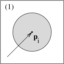
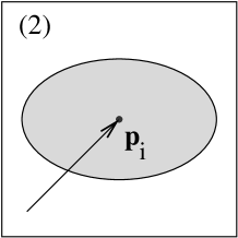
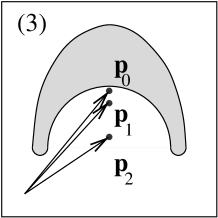
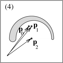
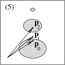
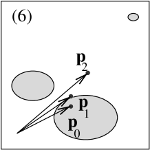
Figure 2: Examples of centroids for a series of simple patterns. The panels (1)–(4) show how the curvature centroids reflect the symmetry of a “cluster”. For patterns consisting of more than one body, the centroids weight the components according to their scalar Minkowski functionals. Note that the patterns in panel (5) and (6) can be discriminated using the centroids, but not by merely employing the scalar Minkowski functionals.

where we use the compact notation ${\vec{\varphi}}\equiv\{V_{i},{\mathbf{V}}_{i}\}$. If $K_{1}$ and $K_{2}$ are arbitrary compact convex bodies, then the union set $K_{1}\cup K_{2}$ is generally no longer convex. However, the right–hand–side of Equation (6) is still well–defined and may be taken as the definition of ${\vec{\varphi}}_{i}(K_{1}\cup K_{2})$. Consequently, additivity allows us to extend the application of the functionals ${\vec{\varphi}}$ to patterns formed by an arbitrary finite union of convex bodies via iteration of Equation (6).
The functionals ${\vec{\varphi}}_{i}$, for $1\leq i\leq d$, depend on the shape of the body $K$; if its surface, $\partial K$, is smooth, with principal curvatures $c_{j}({\mathbf{x}})$, $1\leq j\leq d-1$, then these functionals may be expressed in terms of surface integrals. For instance, in $d=3$, with the surface area element ${\rm d}S({\mathbf{x}})$, and $\vec{z}\equiv(1,{\mathbf{x}})$ we have:

$${\vec{\varphi}}_{1}(K)=\frac{1}{6}\int_{\partial K}\vec{z}{\rm d}S({\mathbf{x}})\;\;\;,\;\;\;{\vec{\varphi}}_{2}(K)=\frac{1}{3\pi}\int_{\partial K}\frac{1}{2}(c_{1}({\mathbf{x}})+c_{2}({\mathbf{x}}))\vec{z}{\rm d}S({\mathbf{x}})\;\;\;,$$ (7)

$${\vec{\varphi}}_{3}(K)=\frac{1}{4\pi}\int_{\partial K}c_{1}({\mathbf{x}})c_{2}({\mathbf{x}})\vec{z}{\rm d}S({\mathbf{x}})\;\;\;.$$

The vector ${\mathbf{V}}_{3}(K)$ is known as the Steiner point of the body $K$. – We list the meanings of the Minkowski functionals and the corresponding vectors in two dimensions in Table 1.
The most prominent feature of the family $\{{\vec{\varphi}}_{i}(\cdot)|0\leq i\leq d\}$ is expressed by Hadwiger’s characterization theorem: Consider the polyconvex ring ${\mathbb{P}}^{d}$ of spatial patterns, defined to comprise the collection of arbitrary finite unions of convex bodies, ${\mathcal{K}}_{N}=\bigcup_{\alpha=1}^{N}K_{\alpha}\in{\mathbb{P}}^{d}$, $N<\infty$, $0\leq\dim K_{\alpha}\leq d$. According to the theorem, any additive, equi– or invariant and conditionally continuous functional $\vec{\Phi}$ on ${\mathbb{P}}^{d}$ is uniquely determined by the linear combination:

$$\vec{\Phi}({\mathcal{K}}_{N})=\sum_{i=0}^{d}a_{i}{\vec{\varphi}}_{i}({\mathcal{K}}_{N}),$$ (8)

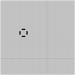
$\leftarrow$

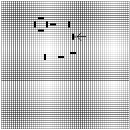
$\rightarrow$

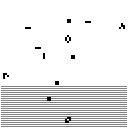
Figure 3: Two initial configurations for the “Game of Life” (middle panel) and the results for the 188th generation (right and left panel). In the initial state, the “thunderbirdfuse” (black cells) is perturbed with the grey cell marked by an arrow. Whereas the “thunderbirdfuse” ends with a “blinker” (left panel), the “perturbed thunderbirdfuse” evolves into a pattern ejecting two gliders (right panel).

with the real coefficients $a_{i}$ independent of the pattern ${\mathcal{K}}_{N}$. In this sense, the family $\{{\vec{\varphi}}_{i}\}$ forms a complete basis of morphometric descriptors.
For the practical analysis of cluster structures, for instance, it is convenient to employ the (curvature) centroids ${\mathbf{p}}_{i}=\left(p_{i}^{x},p_{i}^{y},...\right)={\mathbf{V}}_{i}/V_{i}$, provided $V_{i}\neq 0$, $i=0,..,d$.
Let us consider the series of 2d–clusters shown in Figure 2 to gain some intuition on the kind of information supplied by the functionals ${\vec{\varphi}}_{i}$, and the centroids, in particular.
The clusters (1)–(4) display the effect of symmetry reduction. In the case of the disk (1) and the ellipse (2), the centroids coincide at the symmetry center. However,

Figure 4: The Minkowski functionals for the two “Game of Life” series depicted in Figure 3. We compare the length of the circumference (left panel) and both components of the corresponding centroid (middle and right panel). “thunderbirdfuse”: solid line, “perturbed thunderbirdfuse”: dashed line.

Figure 5: The interplay of all curvature centroids for the second “Game of Life” series depicted in Figure 3 allows us to answer questions on the symmetry and movement of the patterns arising.

$C_{1}$ may be distinguished from $C_{2}$ by the value of the isoperimetric ratio, $I(C_{1})=1$ (which holds only for the disk) and $I(C_{2})>1$, where $I(K)\equiv 4V_{1}^{2}(K)/[\pi V_{0}(K)V_{2}(K)]\geq 1$ for convex bodies. The centroids of $C_{3}$ and $C_{4}$ no longer coincide; in $C_{3}$ they fan out along the single mirror reflection line, whereas in $C_{4}$ they form a triangle. The clusters $C_{5}$ and $C_{6}$ have the same three components, but in different configurations. The scalar Minkowski functionals of both $C_{5}$ and $C_{6}$ differ from the ones of $C_{1}$–$C_{4}$ at least by the value of the Euler characteristic $V_{2}$, which counts here the number of cluster components. But the scalar Minkowski functionals are unsuitable to distinguish $C_{5}$ from $C_{6}$ – additivity implies $V_{i}(C_{5})=V_{i}(C_{6})$ –, whereas the centroids discriminate clearly.
In Figure 3 we illustrate the order parameters using a dynamical cellular automaton generated by the “Game of Life” [5, 7]. We consider two series of patterns, the “thunderbirdfuse”  and a series starting with a slightly perturbed initial configuration of the “thunderbirdfuse”, with one point added (left column of Figure 3). The “thunderbirdfuse” lights consecutively the “blinkers” visible as bars. The temporal sequence as well as the spatial course of the ignitions is reflected by the Minkowski functionals (Figure 4) and the curvature centroids. The evolution terminates with “traffic lights” oscillating with period two and constant values of the scalar and vectorial functionals.
The evolution of the slightly perturbed

Minkowski functional	meaning	corresponding vector
$V_{0}$	surface content	$\int_{K}{\rm d}^{2}V{\mathbf{x}}$
$V_{1}$	one fourth of the length of perimeter	$\frac{1}{4}\int_{\partial K}{\rm d}^{1}S{\mathbf{x}}$
$V_{2}$	Euler characteristic	$\frac{1}{2\pi}\int_{\partial K}{\rm d}^{1}S\;c({\mathbf{x}}){\mathbf{x}}$

Table 1: The meaning of the Minkowski functionals in two dimensions, $c({\mathbf{x}})$ is the local curvature.

“thunderbirdfuse” proceeds rather differently. The early patterns are still comparable; at the time, when the pattern reaches the modified pixel, the perturbed “thunderbirdfuse” grows and attains a constant surface content from generation 188 on. However, as seen from ${\mathbf{p}}_{1}$, the pattern keeps changing by ejecting two gliders visible in the lower right panel. The behaviour of the curvature centroids is shown in Figure 5: The asymmetry of the pattern and its temporal variation (the “gliders” move one cell in diagonal direction within four generations) is clearly recognizable.

3 Applications to galaxy clusters

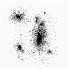
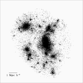
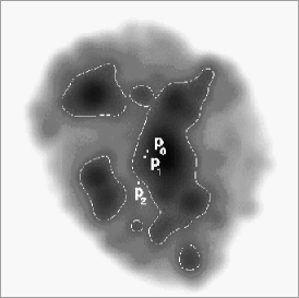
Figure 6: Example for the excursion set approach. The data points of the cluster $\tau$CDM (middle panel) are smoothed using a smoothing length of $0.2h^{-1}{\rm Mpc}$. In the right panel we show the contours and the curvature centroids ${\mathbf{p}}_{i}$ of the excursion set at a density threshold of $u=0.275N/R_{m}^{2}$. Here, $N$ denotes the number of particles within the cluster, $R_{m}$ quantifies the cluster scale via the maximum distance of cluster particles from the cluster center. – $h$ accounts for the uncertainty in the determination of the Hubble constant $H$: $H=100h\frac{km/s}{Mpc}$. – The left panel shows the counterpart of $\tau$CDM, OCDM, which is embedded into an open cosmological model.

Evidently, observational data of galaxies within clusters or X–ray photon maps do not provide from the outset the kind of spatial patterns required for the application of our morphometric tools. To start with, these patterns must first be constructed from the observational data; but there is no canonical way to proceed. Here, we employ two procedures, the excursion set method and the Boolean grain method in order to further illustrate our approach on the basis of simulated and real cluster data.

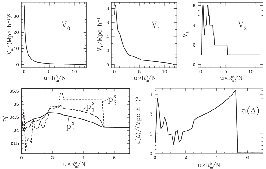
Figure 7: First row: the scalar Minkowski functionals of the cluster depicted in Figure 6 vs. the density threshold $u$ ($u$ is given in units of the mean density within the cluster, $N$ is the number of cluster particles, $R_{m}$ the maximum distance of cluster particles from the center of mass of all cluster particles). Second row: one component of the curvature centroids (left panel) and the area of the triangle spanned by the curvature centroids (right panel).

3.1 The excursion set method

We smooth the projected galaxy positions or the pixels of the X-ray photon maps with a Gaussian kernel. The smoothing length determines the scale of interest. Then we construct the excursion sets and investigate their topology and geometry using the Quermaß vectors and the Minkowski functionals [17].
We illustrate this procedure by comparing two simulated clusters (part of the GIF–simulations, cf. [1, 2]); they start with comparable initial conditions and evolve within different Friedmann–Lemaître models as cosmological background, thus exemplifying the imprint of the background. We demonstrate our method in Figure 6 using the cluster $\tau$CDM from an Einstein–de Sitter model  and a smoothing length of $0.2h^{-1}{\rm Mpc}$. The results of the Minkowski analysis are depicted in Figure 7. We plot the scalar Minkowski functionals vs. the density threshold defining the excursion sets: an averaged and smoothed density profile is encoded in the first Minkowski functional $V_{0}$; a comparison of the square of $V_{1}$ and $V_{0}$ quantifies how crooked the isodensity contours are. The Euler characteristic $V_{2}$ counts the components (minus the number of eventual holes) of this substructure–rich cluster.
The components $p_{i}^{x}$ of the curvature centroids are shown in the fourth panel of Figure 7. They wander in space if the density threshold is varied. This indicates that morphological features are shifting. Another way to make the centroids more illustrative is to consider the triangle spanned by the centroids and to compute its volume and the length of its perimeter (fifth panel of Figure 7). These quantities tell us how symmetric the isodensity contours are.
To compare this cluster to OCDM, its counterpart in a low–density background model, we condense the morphometric information present in the Minkowski functionals and the centroids into a few dimensionless descriptors, by taking into account, that both clusters have different scales and numbers of particles. We define for a function $f$ an average over density thresholds via:

$$\left\langle f\right\rangle_{\rm u}=\frac{1}{u_{max}-u_{min}}\int_{u_{min}}^{u_{max}}{\rm d}uf(u)\;\;\;$$ (9)

$\sigma/h^{-1}{\rm Mpc}$	parameter	definition	$\tau$CDM	OCDM
0.2	c	$\sqrt{\left\langle(\chi-1)^{2}\right\rangle_{\rm u}}$	$3.20$	$2.54$
	$s_{0}/R_{cl}^{2}$	$\left\langle 4V_{0}(\triangle({\mathbf{p}}))\right\rangle_{\rm u}/R_{cl}^{2}$	$8.78\times 10^{-4}$	$6.31\times 10^{-4}$
	${\rm shift}_{0}/R_{cl}$	$\int_{u_{min}}^{u_{max}}\left|\frac{{\rm d}{\mathbf{p}}_{i}}{{\rm d}u}\right|{\rm d}u/R_{cl}$    .	$3.85\times 10^{-1}$	$4.54\times 10^{-1}$

Table 2: The definitions of the condensed descriptors and their values for the clusters $\tau$CDM and OCDM depicted in Figure 6. $4V_{0}(\triangle({\mathbf{p}}))$ is the circumference of the triangle spanned by the curvature centroids. $R_{cl}$ is the scale of the cluster, determined via the area of the convex hull of the cluster $A_{h}$: $\pi R_{cl}^{2}=A_{h}$. $\sigma$ denotes the smoothing length.

and consider the clumpiness, the symmetry parameter and the shift of morphological properties as defined in the third column of Table 2 . These parameters display the imprint of subclumps, the symmetry and shift of the curvature centroid ${\mathbf{p}}_{2}$ and are the larger the more substructure the cluster exhibits. As visible from Table 2, the cluster $\tau$CDM owns more substructure with respect to clumpiness and symmetry. A statistical comparison of these descriptors for larger numbers of clusters simulated in different models yields a typical cluster morphology and may help to constrain the present values of the cosmological parameters [2].

3.2 The Boolean grain method

Figure 8: The cluster population of Cl 0016+161 (left panel) and the associated Boolean grain model with circular windows (right panel). The radius of the Boolean grains is $15$ arcseconds. The units are arcseconds.

Figure 9: The scalar Minkowski functionals for the cluster Cl 0016+161 vs. the radius $R_{D}$ (in arcseconds) of the sampling window. The radius of the grains is fixed ($15^{\prime\prime}$), the Minkowski functionals $V_{i}$ are given in units of arcsec^2-i.

The Boolean grain method decorates each point ${\mathbf{x}}_{i}$ of a point set with a ball $B_{{\mathbf{x}}_{i}}(r)$ of radius $r$. The union set of these balls is diagnosed by computing the Minkowski functionals and centroids as functions of the radius. To probe the morphology of an individual cluster locally, we place a window ${\cal D}$ on the cluster center (the center of the point set) and study the centroids of $\bigcup_{i}B_{{\mathbf{x}}_{i}}(r)\cap{\cal D}$. Inflation of the sampling window ${\cal D}$ allows us to explore different regions of the cluster. We illustrate this method in Figure 8. Note, that also galaxies outside the window contribute .
To provide a concrete example, we investigate the cluster Cl 0016+161 at $z\sim 0.54$ observed by Belloni and Röser [4] with the angular positions and spectral properties of galaxies in a field of $3.5^{\prime}\times 5^{\prime}$ and brighter than $R=23.5{\rm mag}$. Galaxies are

Figure 10: The behaviour of the curvature centroids ($p_{i}^{x}$–component) for the Boolean grain model in Figure 8 vs. the radius of the window (in units of arcseconds). The straight line indicates the cluster center.

considered as cluster members, if their redshifts lie within a predetermined range. We are left with $53$ galaxies in this field, as shown in Figure 8.
We place spherical windows ${\cal D}=B_{R_{D}}({\mathbf{c}})$ of different sizes $R_{D}$ on the center of mass ${\mathbf{c}}$ of the point set. The radius of the Boolean grains is held fixed at $15^{\prime\prime}$. In Figure 9 we show the behaviour of the scalar Minkowski functionals. The area of the union set of balls inside the window ${\cal D}$ increases almost linearly with $R_{D}$. A homogenous galaxy distribution would yield a parabolic dependence, but here the galaxy density drops at larger scales. The small peaks in the Euler characteristic typically arise when two parts of a connected subcluster enter the window simultaneously.
The curvature centroids are more sensitive to geometrical anisotropies. The components $p_{i}^{x}$ are depicted in Figure 10. Two features are clearly visible: the centroids vary when the sampling window grows and, at a fixed scale of the window, significant differences between the curvature centroids arise. The variation of the centroids is clearly correlated with subclusters entering the window, e.g. the wandering of ${\mathbf{p}}_{1}$ and ${\mathbf{p}}_{0}$ towards higher $x$–values reflects the large cluster component in positive $x$–direction of the center.
To analyze the morphology of this cluster more in detail, we simulate a reference model for comparison. The simplest way to generate a reference cluster is an inhomogeneous, but spherically symmetric Poisson process [6]. We determine the projected density profile of the cluster non–parametrically around the center of mass using a binning, and simulate $100$ Poisson clusters using this profile (the method for simulating inhomogeneous point processes is described e.g. in  [22]). The mean Minkowski functionals and the centroids for the model clusters with their r.m.s. fluctuations as well as the results for the real cluster are depicted in Figure 11.
The scalar Minkowski functionals deviate only slightly from the Poisson model. On the other hand, the curvature centroids reveal significant deviations (second row of Figure 11); in particular, the $y$–component of ${\mathbf{p}}_{0}$ (right panel) is shifted away from the true center of mass for relatively small values of the window scale, reflecting the fact, that there are more galaxies above than beneath the cluster center.

Figure 11: The Minkowski functionals (first row) and components of different curvature centroids (second row) for the cluster Cl 0016+161 (solid line) and for a set of Poissonian random clusters following the same density profile as Cl 0016+161 (dashed line) vs. the radius of the Boolean grains in units of arcseconds. The radius of the window is fixed at $69^{\prime\prime}$. The shaded areas indicate the one–$\sigma$–range for the random clusters. Whereas the scalar Minkowski functionals are consistent with the Poisson model, the curvature centroids, especially their $y$–component, reveal a significant deviation from this model.

– To strengthen our conclusions we also simulated the Poisson clusters with a different binning, but the results remained stable. The results demonstrate that the cluster Cl0016+161 exhibits evidential subclustering in comparison with a Poissonian model.

4 Conclusions

The examples discussed in this note support our claim that the method of cluster analysis based on the combination of scalar Minkowski functionals with vectorial centroids furnishes a versatile set of order parameters to sort out essential aspects of cluster morphology such as symmetry, clumpiness, global shape and topology. Our cluster morphometry rests on a solid mathematical basis derived from a few reasonable requirements. In this sense, it allows for a unique morphological description. The construction of patterns from empirical data introduces additional parameters which may be employed advantageously for scale–specific diagnosis. No tacit statistical assumptions are involved.
Finally, we note that these families of morphological measures may be extended further to include tensor–valued Minkowski functionals, which generalize the concept of inertia tensors.
The code to compute the Minkowski functionals and the Quermaß vectors is available on request from the authors.

References

- [1] M. Bartelmann, A. Huss, J. M. Colberg, A. Jenkins, and F. R. Pearce. Arc statistics with realistic cluster potentials. IV. Clusters in different cosmologies. Astron. Astrophys., 330:1–9, 1998.
- [2] C. Beisbart, T. Buchert, M. Bartelmann, J. C. Colberg, and H. Wagner. Application of Quermaß vectors to morphological evolution. 2000. In preparation.
- [3] C. Beisbart, T. Buchert, and H. Wagner. Quermaß vectors and Curvature Centroids: compact morpometry of cosmic Structure. 2000. In preparation.
- [4] P. Belloni and H.-J. Röser. Galaxy population in distant clusters. I. Cl0939+472 (z=0.41) and Cl0016+161 (z=0.54). Ap. J. Suppl., 118:65, 1996.
- [5] E. Berlekamp, J. Conway, and R. Guy. Winning Ways. Academic Press, 1982.
- [6] D. J. Daley and D. Vere-Jones. An introduction to the Theory of Point Processes. Springer Verlag, Berlin, 1988.
- [7] M. Gardner. The fantastic combinations of John Conway’s new solitaire game ”Life”. Scientific American, page 120, Oct. 1970.
- [8] H. Hadwiger and C. Meier. Studien zur vektoriellen Integralgeometrie. Math. Nachr., 56:361–368, 1974.
- [9] H. Hadwiger and R. Schneider. Vektorielle Integralgeometrie. Elemente der Mathematik, 26:49–72, 1971.
- [10] M. Kerscher, J. Schmalzing, T. Buchert, and H. Wagner. Fluctuations in the 1.2 Jy galaxy catalogue. Astron. Astrophys., 333:1–12, 1998.
- [11] M. Kerscher, J. Schmalzing, J. Retzlaff, S. Borgani, T. Buchert, S. Gottlöber, V. Müller, M. Plionis, and H. Wagner. Minkowski functionals of Abell/ACO clusters. Mon. Not. R. Astron. Soc., 284:73–84, 1997.
- [12] P. McMullen and R. Schneider. Valuations on convex bodies. In P. M. Gruber and J. M. Wills, editors, Convexity and its applications, pages 170–247. Birkhäuser, Basel, 1983.
- [13] K. Mecke. Morphological characterization of patterns in reaction–diffusion systems. Phys. Rev. D, 53:4794–4800, 1996.
- [14] K. Mecke, T. Buchert, and H. Wagner. Robust morphological measures for large-scale structure in the Universe. Astron. Astrophys., 288:697, 1994.
- [15] K. Mecke and V. Sofonea. Morphology of spinodal decomposition. Phys. Rev. D, 56:R3761–R3764, 1997.
- [16] V. Sahni, B. S. Sathyaprakash, and S. F. Shandarin. Shapefinders: a new shape diagnostic for large-scale structure. Ap. J. Lett., 459:5, 1998.
- [17] J. Schmalzing and T. Buchert. Beyond genus statistics: a unifying approach to the morphology of cosmic structure. Ap. J. Lett., 482:L1, 1997.
- [18] J. Schmalzing, T. Buchert, A. L. Melott, V. Sahni, B. S. Sathyaprakash, and S. F. Shandarin. ”disentangling the cosmic web. i. morphology of isodensity contours”. Ap. J., 526:568–578, 1999.
- [19] J. Schmalzing and K. Gorski. Minkowski functionals used in the morphological analysis of cosmic microwave background anisotropy maps. Mon. Not. R. Astron. Soc., 297:355, 1998.
- [20] R. Schneider. Krümmungsschwerpunkte konvexer Körper (i). Abh. Math. Sem. Univ. Hamburg, 37:112–132, 1972.
- [21] R. Schneider. Krümmungsschwerpunkte konvexer Körper (ii). Abh. Math. Sem. Univ. Hamburg, 37:202–217, 1972.
- [22] D. Stoyan and H. Stoyan. Fractals, Random Shapes and Point Fields. John Wiley & Sons, Chichester, 1994.