Large scale dynamos with ambipolar diffusion nonlinearity

Abstract

It is shown that ambipolar diffusion as a toy nonlinearity leads to very similar behaviour of large scale turbulent dynamos as full MHD. This is demonstrated using both direct simulations in a periodic box and a closure model for the magnetic correlation functions applicable to infinite space. Large scale fields develop via a nonlocal inverse cascade as described by the alpha-effect. However, because magnetic helicity can only change on a resistive timescale, the time it takes to organize the field into large scales increases with magnetic Reynolds number.

1 Ambipolar diffusion as a toy nonlinearity

In this Letter we test and exploit the idea that the exact type of nonlinearity in the MHD equations is unessential as far as the nature of large scale field generation is concerned. At first glance this may seem rather surprising, especially if one pictures large scale field generation as the result of an inverse cascade process (Frisch et al. 1975, Pouquet et al. 1976). Like the direct cascade in Kolmogorov turbulence, the inverse cascade is accomplished by nonlinear interactions, suggesting that nonlinearity is important. However, a special type of inverse cascade is the strongly nonlocal inverse cascade process, which is usually referred to as the ‘alpha-effect’; see Moffatt (1978) and Krause & Rädler (1980). This effect exists already in linear (kinematic) theory.

Until recently it was unclear which, if any, of the two effects (inverse cascade in the local sense or the $\alpha$-effect) played the dominant role in large scale field generation as seen in simulations (e.g. Glatzmaier & Roberts 1995, Brandenburg et al. 1995, Ziegler & Rüdiger 2000) or in astrophysical bodies (stars, galaxies, accretion discs). A strong indication that it is actually the $\alpha$-effect (i.e. the strongly nonlocal inverse cascade) that is responsible for large scale field generation, comes from detailed analysis of recent three-dimensional simulations of forced isotropic non-mirror symmetric turbulence (Brandenburg 2000, hereafter B2000). In those simulations a strong and nearly force-free magnetic field was produced, and most of the energy supply to this field was found to come from the forcing scale of the turbulence.

In the absence of nonlinearity, however, the field seen in the simulations of B2000 became quickly swamped by magnetic fields at smaller scales. In that sense a purely kinematic large scale turbulent dynamo is impossible! Any hope for analytic progress is therefore slim. However, the model of Subramanian (1997, 1999) is an exception. Subramanian (1997; hereafter S97) extended the kinematic models of of Kazantsev (1968) and Vainshtein & Kitchatinov (1986) by including ambipolar diffusion (in the strong coupling approximation) as a nonlinearity. Under the common assumption that the velocity is delta-correlated in time, S97 derived a nonlinear equation for the evolution of the correlation functions of magnetic field and magnetic helicity. Although the models of Kazantsev (1968) and Novikov et al. (1983) are usually known to describe small-scale field generation, Subramanian (1999; hereafter S99) found that in the presence of fluid helicity there is the possibility of tunnelling of bound-states corresponding to small scales to unbounded states corresponding to large scale fields, which are force-free.

In this Letter we present numerical solutions to the closure model of S99. We stress that we do not advocate ambipolar diffusion (AD) as being dominant over the usual feedback from the Lorentz force in the momentum equation. Instead, our motivation is to establish a useful toy model to study effects of nonlinearity in dynamos. Our numerical solutions may provide guidance for further analytic treatment of these equations in parameter regimes otherwise inaccessible. We begin however by considering first solutions of the fully three-dimensional MHD equations in a periodic box using AD as the only nonlinearity.

2 Box simulations for a finite system

In this section we adopt the MHD equations for an isothermal compressible gas, driven by a given body force $f$, in the presence of AD, but ignoring the Lorentz force

$${{\rm D}\,{}\ln\rho\over{\rm D}\,{}t}=-\mbox{\boldmath$\nabla$}{}\cdot\mbox{\boldmath$u$}{},$$ (1)

$${{\rm D}\,{}\mbox{\boldmath$u$}{}\over{\rm D}\,{}t}=-c_{\rm s}^{2}\mbox{\boldmath$\nabla$}{}\ln\rho+{\mu\over\rho}(\nabla^{2}\mbox{\boldmath$u$}{}+{\textstyle{1\over 3}}\mbox{\boldmath$\nabla$}{}\mbox{\boldmath$\nabla$}{}\cdot\mbox{\boldmath$u$}{})+\mbox{\boldmath$f$}{},$$ (2)

$${\partial\mbox{\boldmath$A$}{}\over\partial t}=(\mbox{\boldmath$u$}{}+\mbox{\boldmath$u$}{}_{\rm D})\times\mbox{\boldmath$B$}{}-\eta\mu_{0}\mbox{\boldmath$J$}{},$$ (3)

where ${\rm D}/{\rm D}t=\partial/\partial t+\mbox{\boldmath$u$}{}\cdot\mbox{\boldmath$\nabla$}{}$ is the advective derivative, $\mbox{\boldmath$B$}{}=\mbox{\boldmath$\nabla$}{}\times\mbox{\boldmath$A$}{}$ is the magnetic field, $\mbox{\boldmath$J$}{}=\mbox{\boldmath$\nabla$}{}\times\mbox{\boldmath$B$}{}/\mu_{0}$ is the current density, and $f$ is the random forcing function as specified in B2000. The nonlinear drift velocity $\mbox{\boldmath$u$}{}_{\rm D}$ due to AD can be written as $\mbox{\boldmath$u$}{}_{\rm D}=a\,\mbox{\boldmath$J$}{}\times\mbox{\boldmath$B$}{}$. We use nondimensional units where $c_{\rm s}=k_{1}=\rho_{0}=\mu_{0}=1$. Here, $c_{\rm s}$ is the sound speed, $k_{1}$ the smallest wavenumber of the box (so its size is $2\pi$), $\rho_{0}$ is the mean density, and $\mu_{0}$ is the vacuum permeability. Since AD is the only nonlinearity in Eq. (3) we can always normalize $B$ such that $a=1$.

The model presented here is similar to Run 3 of B2000, where $\mu=\eta=2\times 10^{-3}$. With a root-mean-square velocity of around 0.3 the magnetic Reynolds number based on the size of the box is around 1000. The forcing wavenumber $k_{\rm f}$ is chosen to be 5. In Fig. 1 we show a grey scale representation of a slice of the magnetic field and the current density at $t=337$. Note the presence of a large scale magnetic field that varies in the $z$-direction. In Fig. 2 we show the spectra of magnetic and kinetic energies. The peak of magnetic energy at $k=1$ shows the development of large scale magnetic fields. Further, the current density is concentrated into narrow filamentary structures, typical of AD (see Brandenburg & Zweibel 1994).

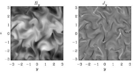
Figure 1: Images of $B_{y}$ and $J_{y}$ in an arbitrarily chosen $yz$ plane. $120^{3}$ meshpoints, $t=337$.

Unfortunately, the severity of the diffusive timestep limit, $\delta t\leq 0.16\delta x^{2}/\eta_{\rm AD}$, where $\eta_{\rm AD}=a\mbox{\boldmath$B$}{}^{2}$, prevented us from running much longer at high resolution ($120^{3}$ meshpoints). For $60^{3}$ meshpoints this limit is unimportant, and so we were able to run until $t=900$, a time when the large scale field was much more clearly defined. In the inset of Fig. 2, we show the evolution for such a case, but with a forcing at $k_{\rm f}=10$ (giving larger scale separation). Note again the peak of $E_{M}$ at $k=1$ and also the suppression of magnetic field at the next smaller scale, corresponding to $k\geq 2$. Both these features are very similar to the magnetic field evolution in the case with full Lorentz force and without AD (Figs 3 and 17 of B2000).

Figure 2: Spectra of magnetic energy (solid lines), kinetic energy (dash-dotted line), magnetic helicity (normalized by $k/2$; dashed line) for the run shown in Fig. 1. The inset shows spectra of a run with forcing at $k=10$ and $60^{3}$ meshpoints for different times till $t=900$.

Our main conclusion from these results is first of all that large scale field generation works in spite of AD, contrary to earlier suggestions that AD might suppress the large scale dynamo process (Kulsrud & Anderson 1992). Secondly, AD provides a nonlinear saturation mechanism for the magnetic field at all scales, except for the scale of the box, where a force-free field develops for which $\mbox{\boldmath$u$}{}_{\rm D}$ vanishes. Like in the simulations of B2000 this provides a ‘self-cleaning’ mechanism, without which the field would be dominated by contributions from small scales.

Having established the close similarity between models with AD versus full Lorentz force as nonlinearity, we now move on to discuss the nonlinear closure model of S99 with AD as a ‘toy’ nonlinearity.

3 Closure model for an infinite system

Under the assumptions that the velocity is delta-correlated in time and the magnetic field is a gaussian random field S97 derived equations for the longitudinal correlation function $M(r,t)$ and the correlation function for magnetic helicity density, $N(r,t)$. The velocity is represented by a longitudinal correlation function $T(r)$ and a correlation function for the kinetic helicity density, $C(r)$. We change somewhat the notation of S99 and define the operators

$$\tilde{D}(\cdot)={1\over r^{4}}\,{\partial\over\partial r}\left(r^{4}\cdot\right),\quad D(\cdot)={\partial\over\partial r}(\cdot),$$ (4)

so the closure equations can be written as

$$\dot{M}=2\tilde{D}(\eta_{\rm T}DM)+2GM+4\alpha H,$$ (5)

$$\dot{N}=-2\eta_{\rm T}H+\alpha M,$$ (6)

where $H=-\tilde{D}DN$ is the correlation function of the current helicity, $G=-\tilde{D}DT$ is the effective induction,

$$\alpha=\alpha_{0}(r)+4aH(0,t)$$ (7)

$$\eta_{\rm T}=\eta+\eta_{0}(r)+2aM(0,t)$$ (8)

are functions resembling the usual $\alpha$-effect and the total magnetic diffusivity. Here $\alpha_{0}(r)=-2[C(0)-C(r)]$ and $\eta_{0}(r)=T(0)-T(r)$. Note that at large scales

$$\alpha_{\infty}\equiv\alpha(r\rightarrow\infty)=-{\textstyle{1\over 3}}\tau\langle\mbox{\boldmath$\omega$}{}\cdot\mbox{\boldmath$u$}{}\rangle+{\textstyle{1\over 3}}\tau_{\rm AD}\langle\mbox{\boldmath$J$}{}\cdot\mbox{\boldmath$B$}{}\rangle/\rho_{0}$$ (9)

$$\eta_{\infty}\equiv\eta_{\rm T}(r\rightarrow\infty)={\textstyle{1\over 3}}\tau\langle\mbox{\boldmath$u$}{}^{2}\rangle+{\textstyle{1\over 3}}\tau_{\rm AD}\langle\mbox{\boldmath$B$}{}^{2}\rangle/\mu_{0}\rho_{0},$$ (10)

where $\tau_{\rm AD}=2a\rho_{0}$. Expression (9) is very similar to the $\alpha$-suppression formula first found by Pouquet et al. (1976). Here $\alpha$ and $\eta_{\rm T}$ are scale dependent (i.e. they are largest on large scales) and, in addition, both are affected by AD.

We construct $T(r)$ and $C(r)$ from an analytic approximation of the kinetic energy and helicity spectra, $E_{\rm K}(k)$ and $H_{\rm K}(k)$, respectively. Zero velocity at large scales means that $E_{K}(k)\sim k^{4}$ for $k\rightarrow 0$. At some wavenumber $k=k_{\rm f}$ the spectrum turns to a $k^{-5/3}$ Kolmogorov spectrum, followed by an exponential cutoff, so we take

$$E_{\rm K}(k)={E_{0}\,(k/k_{\rm f})^{4}\over 1+(k/k_{\rm f})^{17/3}}\,\exp(-k/k_{\rm d}).$$ (11)

We use parameters representative of the simulations of B2000, so $E_{0}=0.01$, $k_{\rm f}=5$ and $k_{\rm d}=25$. Like in B2000 we assume the turbulence fully helical, so $H_{\rm K}=2kE_{\rm K}$ (e.g. Moffatt 1978). The correlation functions $T(r)$ and $C(r)$ are then obtained via

$$T(r)={2\over\tau}\int_{0}^{\infty}E(k)\,{j_{1}(kr)\over kr}\,{\rm d}{}k\equiv{\cal I}(E(k)),$$ (12)

and $C(r)={\cal I}(F(k))/4$, where $j_{1}(x)=(\sin x-x\cos x)/x^{2}$ and $\tau$ is the correlation time. (We use $\tau=4$, representative of the kinematic stage of Run 3 of B2000.)

We solve Eqs. (5) and (6) using second order finite differences and a third order time step on a uniform mesh in $0<x<L$ with up to 10,000 meshpoints and $L=10\pi$, which is large enough so that the outer boundary does not matter. In the absence of helicity, $C=0$, and without nonlinearity, $a=0$, we recover the model of Novikov et al. (1983). The critical magnetic Reynolds number based on the forcing scale is around 60. In the presence of helicity this critical Reynolds number decreases, confirming the general result that helicity promotes dynamo action (cf. Kim & Hughes 1997, S99). In the presence of nonlinearity the exponential growth of the magnetic field terminates when the magnetic energy becomes large. After that point the magnetic energy continues however to increase nearly linearly. Unlike the case of the periodic box (Sect. 2) the magnetic field can here extend to larger and larger scales; see Fig. 3. The corresponding magnetic energy spectra,

$$E_{\rm M}(k,t)={1\over\pi}\int_{0}^{L}M(r,t)\,(kr)^{3}\,j_{1}(kr)\,{\rm d}{}k,$$ (13)

are shown in Fig. 4.

Figure 3: Evolution of magnetic correlation functions for different times. The correlation function of the magnetic helicity is shown in the inset. $\eta=10^{-3}$.

Figure 4: Evolution of magnetic energy spectra. Note the propagation of magnetic helicity and energy to progressively larger scales. The $k^{-2}$ slope is given for orientation.

The resulting magnetic field is strongly helical and the magnetic helicity spectra (not shown) satisfy $H_{\rm M}\mathrel{\mathchoice{\vbox{\offinterlineskip\halign{\hfil$\displaystyle#$\hfil\cr<\cr\sim\cr}}}{\vbox{\offinterlineskip\halign{\hfil$\textstyle#$\hfil\cr<\cr\sim\cr}}}{\vbox{\offinterlineskip\halign{\hfil$\scriptstyle#$\hfil\cr<\cr\sim\cr}}}{\vbox{\offinterlineskip\halign{\hfil$\scriptscriptstyle#$\hfil\cr<\cr\sim\cr}}}}(2/k)E_{\rm M}$. The development of a helicity wave travelling towards smaller and smaller $k$, as seen in Fig. 4, is in agreement with the closure model of Pouquet et al. (1976). In the following we shall address the question of whether or not the growth of this large scale field depends on the magnetic Reynolds number (as in B2000). We have checked that to a very good approximation the wavenumber of the peak is given by

$$k_{\rm peak}(t)\approx\alpha_{\infty}(t)/\eta_{\infty}(t).$$ (14)

This result is familiar from mean-field dynamo theory (see also S99) and is consistent with simulations (B2000, section 3.5). Note that here $k_{\rm peak}$ decreases with time because $\alpha_{\infty}$ tends to a finite limit and $\eta_{\infty}$ increases. (This is not the case in the box calculations where $k_{\rm peak}\geq 2\pi/L$.)

4 Resistively limited growth on large scales

In an unbounded system the magnetic helicity, $\langle\mbox{\boldmath$A$}{}\cdot\mbox{\boldmath$B$}{}\rangle=6N(0,t)$, can only change if there is microscopic magnetic diffusion and finite current helicity, $\langle\mbox{\boldmath$J$}{}\cdot\mbox{\boldmath$B$}{}\rangle=6H(0,t)$,

$${\rm d}{}\langle\mbox{\boldmath$A$}{}\cdot\mbox{\boldmath$B$}{}\rangle/{\rm d}{}t=-2\eta\langle\mbox{\boldmath$J$}{}\cdot\mbox{\boldmath$B$}{}\rangle.$$ (15)

The closure model of S97 and S99 also satisfies this constraint. (Note that ambipolar and/or turbulent diffusion do not enter!) As explained in B2000, this constraint limits the speed at which the large scale field can grow, but not its final amplitude. One way to relax this constraint is if there is a flux of helicity through open boundaries (Blackman & Field 2000, Kleeorin et al. 2000), which may be important in astrophysical bodies with boundaries. Here, however, we consider an infinite system.

In Fig. 5 we show that, after some time $t=t_{\rm s}$, $\langle\mbox{\boldmath$J$}{}\cdot\mbox{\boldmath$B$}{}\rangle$ reaches a finite value. This value increases somewhat as $\eta$ is decreased. In all cases, however, $\langle\mbox{\boldmath$J$}{}\cdot\mbox{\boldmath$B$}{}\rangle$ stays below $\langle\mbox{\boldmath$\omega$}{}\cdot\mbox{\boldmath$u$}{}\rangle(2\tau/a)$, so that $|\alpha_{\infty}|$ remains finite; see (9). A constant $\langle\mbox{\boldmath$J$}{}\cdot\mbox{\boldmath$B$}{}\rangle$ implies that $\langle\mbox{\boldmath$A$}{}\cdot\mbox{\boldmath$B$}{}\rangle$ grows linearly at a rate proportional to $\eta$. However, since the large scale field is helical, and since most of the magnetic energy is by now (after $t=t_{\rm s}$) in the large scales, the magnetic energy is proportional to $\langle\mbox{\boldmath$B$}{}^{2}\rangle\approx k_{\rm peak}\langle\mbox{\boldmath$A$}{}\cdot\mbox{\boldmath$B$}{}\rangle$, and can therefore only continue to grow at a resistively limited rate, see Fig. 5.

Figure 5: (a) Evolution of $\langle\mbox{\boldmath$J$}{}\cdot\mbox{\boldmath$B$}{}\rangle$ for different values of $\eta$. The corresponding value of $\alpha_{\infty}$ is shown on the right hand side of the plot. (b) The evolution of magnetic energy for the same values of $\eta$.

5 Conclusions

Our results have shown that ambipolar diffusion (AD) provides a useful model for nonlinearity, enabling analytic (or semi-analytic) progress to be made in understanding nonlinear dynamos. There are two key features that are shared both by this model and by the full MHD equations: (i) large scale fields are the result of a nonlocal inverse cascade as described by the $\alpha$-effect, and (ii) after some initial saturation phase the large scale field continues to grow at a rate limited by magnetic diffusion. We reiterate that in astrophysical bodies the presence of open boundaries may relax the helicity constraint. Furthermore, the presence of large scale shear or differential rotation provides a means of amplifying toroidal magnetic fields quite independently of magnetic helicity, but this still requires poloidal fields for which the above conclusions hold.

- (1) Blackman, E. G., & Field, G. F. 2000, ApJ 534, 984
- (2) Brandenburg, A., astro-ph/0006186 (B2000)
- (3) Brandenburg, A., & Zweibel, E. G. 1994, ApJ (Letters) 427, L91
- (4) Brandenburg, A., Nordlund, Å., Stein, R. F., & Torkelsson, U. 1995, ApJ 446, 741
- (5) Frisch, U., Pouquet, A., Léorat, J., & Mazure, A. 1975, J. Fluid Mech. 68, 769
- (6) Glatzmaier, G. A., & Roberts, P. H. 1995, Nat 377, 203
- (7) Kazantsev, A. P. 1968, Sov. Phys. JETP 26, 1031
- (8) Kim, E., & Hughes, D. W. 1997, Phys. Lett. 236, 211
- (9) Kleeorin, N. I, Moss, D., Rogachevskii, I., & Sokoloff, D. 2000 A&A
- (10) Krause, F., & Rädler, K.-H. 1980, Mean-Field Magnetohydrodynamics and Dynamo Theory (Pergamon Press, Oxford)
- (11) Kulsrud, R. M., & Anderson, S. W. 1992, ApJ 396, 606
- (12) Moffatt, H. K. 1978, Magnetic Field Generation in Electrically Conducting Fluids (Cambridge University Press, Cambridge)
- (13) Novikov, V. G., Ruzmaikin, A. A., & Sokoloff, D. D. 1983, Sov. Phys. JETP 58, 527
- (14) Pouquet, A., Frisch, U., & Léorat, J. 1976, J. Fluid Mech. 77, 321
- (15) Subramanian, K. 1997 astro-ph/9708216 (S97)
- (16) Subramanian, K. 1999, Phys. Rev. Lett. 83, 2957 (S99)
- (17) Vainshtein, S. I., & Kitchatinov, L. L. 1986, J. Fluid Mech. 168, 73
- (18) Ziegler, U., & Rüdiger, G. 2000, A&A 356, 1141