Computational AstroStatistics: Fast Algorithms and Efficient Statistics for Density Estimation in Large Astronomical Datasets

Abstract

We present initial results on the use of Mixture Models for density estimation in large astronomical databases. We provide herein both the theoretical and experimental background for using a mixture model of Gaussians based on the Expectation Maximization (EM) Algorithm. Applying these analyses to simulated data sets we show that the EM algorithm – using the both the AIC & BIC penalized likelihood to score the fit – can out-perform the best kernel density estimate of the distribution while requiring no “fine–tuning” of the input algorithm parameters. We find that EM can accurately recover the underlying density distribution from point processes thus providing an efficient adaptive smoothing method for astronomical source catalogs. To demonstrate the general application of this statistic to astrophysical problems we consider two cases of density estimation; the clustering of galaxies in redshift space and the clustering of stars in color space. From these data we show that EM provides an adaptive smoothing of the distribution of galaxies in redshift space (describing accurately both the small and large-scale features within the data) and a means of identifying outliers in multi–dimensional color–color space (e.g. for the identification of high redshift QSOs). Automated tools such as those based on the EM algorithm will be needed in the analysis of the next generation of astronomical catalogs (2MASS, FIRST, PLANCK, SDSS) and ultimately in in the development of the National Virtual Observatory.

Department of Physics, Carnegie Mellon University, 5000 Forbes Avenue, Pittsburgh, PA-15213

Department of Physics & Astronomy, University of Pittsburgh

Robotics Institute & the Computer Science Department, Carnegie Mellon University, 5000 Forbes Avenue, Pittsburgh, PA-15213

Department of Statistics, Carnegie Mellon University, 5000 Forbes Avenue, Pittsburgh, PA-15213

1. Introduction

With recent technological advances in wide field survey astronomy it has now become possible to map the distribution of galaxies and stars within the local and distant Universe across a wide full spectral range (from X-rays through to the radio) e.g. FIRST, MAP, Chandra, HST, ROSAT, SDSS, 2dF, Planck. In isolation, the scientific returns from these new data sets will be enormous, combined however, these data will represent a new paradigm for how we undertake astrophysical research. They present the opportunity to create a “Virtual Observatory” that will enable a user to seamlessly analyze and interact with a multi-frequency digital map of the sky. While the wealth of information contained within these new surveys is clear, the questions we must address is how to we efficiently analyze these massive and intrinsically multidimensional data sets. Standard statistical approaches do not easily scale to the regime of 10⁸ data points and 100’s of dimensions.

Therefore, we have formed a collaboration of computer scientists, statisticans and astrophysics to address this problem through the development of fast and efficient statistical algorithms that scale to many dimensions and large datasets like those found in astronomy. In this volume, we present outlines of our on–going research including the use of tree algorithms for fast n–point correlation functions (Schneider et al.), non-parametric density estimations (Genovese et al.) and data visualisation (Welling et al.). In this paper, we present initial results from the application of Mixture Models to the general problem of density estimation in astrophysics; the reader is referred to Connolly et al. (2000, in preparation) for the full details of the theory, the algorithm and our results.

2. Outline of the Algorithm

Let $X^{n}=(X_{1},\ldots,X_{n})$ represent the data. Each $X_{i}$ is a $d$-dimensional vector giving, for example, the location of the $i^{th}$ galaxy. We assume that $X_{i}$ takes values in a set $A$ where $A$ is a patch of the sky from which we have observed. We regard $X_{i}$ as having been drawn from a probability distribution with probability density function $f$. This means that $f\geq 0$, $\int_{A}f(x)dx=1$ and the proportion of galaxies in a region $B$ is given by $Pr(X_{i}\in B)=\int_{B}f(x)dx.$ In other words, $f$ is the the normalized galaxy density and the proportion of galaxies in a region $B$ is just the integral of $f$ over $B$. Our goal is to estimate $f$ from the observed data $X^{n}$.

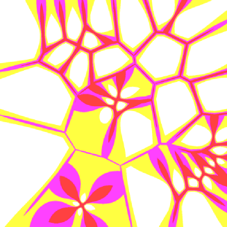
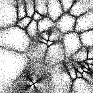
Figure 1.: A comparison of the fixed kernel and our EM density estimation. Top left panel is the simulated Voronoi density distribution while top right shows 100,000 data points draw from this distribution.

The density $f$ is assumed to be of the form

$$f(x;\theta_{k})=p_{0}U(x)+\sum_{j=1}^{k}p_{j}\phi(x;\mu_{j},\Sigma_{j})$$ (1)

where $\phi(x;\mu,\Sigma)$ denotes a $d$-dimensional Gaussian with mean $\mu$ and covariance $\Sigma$:

$$\phi(x;\mu,\Sigma)=\frac{1}{(2\pi)^{d/2}|\Sigma|^{1/2}}\exp\left\{-\frac{1}{2}(x-\mu)^{T}\Sigma^{-1}(x-\mu)\right\},$$

and $U(\cdot)$ is a uniform density over $A$ i.e. $U(x)=1/V$ for all $x\in A$, where $V$ is the volume of $A$. The unknown parameters in this model are $k$ (the number of Gaussians) and $\theta_{k}=(p,\mu,\Sigma)$ where $p=(p_{0},\ldots,p_{k})$, $\mu=(\mu_{1},\ldots,\mu_{k})$ and $\Sigma=(\Sigma_{1},\ldots,\Sigma_{k})$. Here, $p_{j}\geq 0$ for all $j$ and $\sum_{j=0}^{k}p_{j}=1$. This model is called a mixture of Gaussians (with a uniform component). The parameter $k$ controls the complexity of the density $f$. Larger values of $k$ allow us to approximate very complex densities $f$ but also entail estimating many more parameters. It is important to emphasize that we are not assuming that the true density $f$ is exactly of the form (Eqn. 1). It suffices that $f$ can be approximated by such a distribution of Gaussians. For large enough $k$, nearly any density can be approximated by such a distribution (see Roeder & Wasserman 1997).

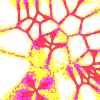
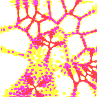
Figure 2.: The resulting density estimates from the data in Figure 1: fixed kernel (left) and EM+AIC (left)

2.1. The EM Algorithm

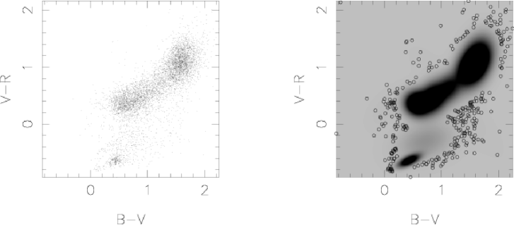
Figure 3.: The application of our algorithm to density estimation in color space. The left panel shows the distribution of $B-V$ and $V-R$ colors of stellar sources while the right hand panel shows the density distribution, as a grayscale, of these sources derived from our algorithm (using AIC). The open circles are the 5% of the data that is least likely to be drawn from this distribution.

How do we find the maximum likelihood estimate of $\theta_{k}$ i.e. $\hat{\theta}$? (We assume for the moment that $k$ is fixed and known.) The usual method for finding $\hat{\theta}$ is the EM (expectation maximization) algorithm. We can regard each data point $X_{i}$ as arising from one of the $k$ components of the mixture. Let $G=(G_{1},\ldots,G_{k})$ where $G_{i}=j$ means that $X_{i}$ came from the $j^{th}$ component of the mixture. We do not observe $G$ so $G$ is called a latent (or hidden) variable. Let $\ell_{c}$ be the log-likelihood if we knew the latent labels $G$. The function $\ell_{c}$ is called the complete-data log-likelihood. The EM algorithm proceeds as follows. We begin with starting values $\theta_{0}$. We compute $Q_{0}=E(\ell_{c};\theta_{0})$, the expectation of $\ell_{c}$, treating $G$ as random, with the parameters fixed at $\theta_{0}$. Next we maximize $Q_{0}$ over $\theta$ to obtain a new estimate $\theta_{1}$. We then compute $Q_{1}=E(\ell_{c};\theta_{1})$ and continue this process. Thus we obtain a sequence of estimates $\theta_{0},\theta_{1},\ldots$ which are known to converge to a local maximum of the likelihood. See Connolly et al. (2000) for more details.

Above, we have assumed that $k$ is known. One approach of choosing $k$ from the data is to sequentially test a series of hypotheses i.e. test the density estimation using $k$ versus the one with $k+1$ and repeat for various $k$.The usual test for comparing such hypotheses is called the “likelihood ratio test” which compares the value of the maximized log-likelihood under the two hypotheses. This approach is infeasible for large data sets where $k$ might be huge. Also, this requires knowing the distribution of the likelihood ratio statistic which is not known. As an alternative (see Connolly et al. 2000 for the explanation), we use two common penalized log–likelihoods to test these two hypotheses, namely Akaike Information Criterion (AIC) and Bayesian Information Criterion (BIC) which take the general form of $\ell(\hat{\theta}_{k})-\lambda_{k}R_{k}$ where $R_{k}$ is the number of parameters in the $k^{th}$ model. For AIC $\lambda_{k}=1$ while $\lambda_{k}=\log n/2$ gives the BIC criterion. See Connolly et al. (2000) for a full explanation.

Given the definition of the EM algorithm and the criteria for determining the number of components to the model using AIC and BIC we must now address how do we apply this formalism to massive multi–dimensional astronomical datasets. In its conventional implementation, each iteration of EM visits every data point pair, meaning $kR$ evaluations of a $M$-dimensional Gaussian, where $R$ is the number of data-points and $k$ is the number of components in the mixture. It thus needs $O(M^{2}kR)$ arithmetic operations per iteration. For data sets with 100s of attributes and millions of records such a scaling will clearly limit the application of the EM technique. We must therefore develop an algorithmic approach that reduces the cost and number of operations required to construct the mixture model. To do this, we have used Multi-resolution KD-trees to gain impressive speed–ups for the numerous range–searches involved in computing the fits of these $k$ gaussians to the data. Such tree algorithms are discussed in detail by Schneider et al. in this volume.

3. Applications to Astrophysical Problems

To test the sensitivity of the Mixture Model density estimation to the heirarchical clustering in the universe, and thus determine if it is better than present, more traditional, astronomical methods of density estimations, we have tested our algorithm using simulated data generated from a Voronoi Tessellation since this mimics the observed distribution of filaments and sheets of galaxies in the universe. In Figure 1, we present the underlying Voronoi density map we have constructed; this is the “truth” in our simulation. From this distribution we derive a set of 100,000 data points to represent a mock 2-dimensional galaxy catalog.

We have applied the EM algorithm (with both the AIC and BIC criteria) and a standard fixed kernel density estimator to these point-like data sets in order to reproduce the original density field. The latter involved finely binning the data and smoothing the subsequent grid with a binned Gaussian filter of fixed bandwidth which was chosen by hand to minimize the Kullback-Leibler distance ($D(f,g)=\int f(x)\log f(x)/g(x)dx$) between the resulting smoothed map and the true underlying density distribution. Clearly, we have taken the optimal situation for the fixed kernel estimator since we have selected it’s bandwidth to ensure as close a representation of the true density distribution as possible. This would not be the case in reality.

In Figure 2, we show the reconstructed density field using the fixed kernel and EM algorithm (AIC). As we would expect the fixed kernel technique provides an accurate representation of the overall density field. The kernel density map suffers, however, when we consider features that are thinner than the width of the kernel. Such filamentary structures are over-smoothed and have their significance reduced. In contrast the EM algorithm attempts to adapt to the size of the structures it is trying to reconstruct. The right panel shows that where narrow filamentary structures exist the algorithm places a large number of small Gaussians. For extended, low frequency, components larger Gaussians are applied. For the fixed kernel estimator, we have a measured KL divergence of 0.074 between the final smoothed map and the true underlying density map (remember, this is the smallest KL measurement by design). For the EM AIC density map we measure a KL divergence of 0.067 which is lower than the best fixed kernel KL score thus immediately illustrating the power of the EM methodology. We have not afforded the same prior knowledge to the EM measurement – i.e.  hand–tune it so as to minimize the KL divergence – yet we have beaten the kernel estimator.

We have extended the analysis above to real astronomical data e.g. the the distribution of 6298 stellar sources in the B-V and V-R color space (with R$<$22) taken from a 1 sq degree multicolor photometric survey of Szokoly et al. (2000). In this case, the mixture model density distribution naturally provides a probability density map that a stellar object drawn at random from the observed distribution of stars would have a particular set of B-V – V-R colors. We can now assign a probability to each star in the original data that describes the likelihood that it arises from the overall distribution of the stellar locus. We can then rank order all sources based on the likelihood that they were drawn from the parent distribution. The right panel of Figure 3 shows the colors of the 5% of sources with the lowest probabilities. These sources lie preferentially away from the stellar locus and thus can be used to find high redshift quasars as outliers to color–space. As we increase the cut in probability the colors of the selected sources move progressively closer to the stellar locus.

The advantage of the EM approach over standard color selection techniques is that we identify objects based on the probability that they lie away from the stellar locus (i.e. we do not need to make orthogonal cuts in color space as the probability contours will trace accurately the true distribution of colors). While for two dimensions this is a relatively trivial statement as it is straightforward to identify regions in color–color space that lie away from the stellar locus (without being restricted to orthogonal cuts in color-color space) this is not the case when we move to higher dimensional data. For four and more colors we lose the ability to visualize the data with out projecting it down on to a lower dimensionality subspace (i.e. we can only display easily 3 dimensional data). In practice we are, therefore, limited to defining cuts in these subspaces which may not map to the true multidimensional nature of the data. The EM algorithm does not suffer from these disadvantages as a probability density distribution can be defined in an arbitrary number of dimensions. It, therefore, provides a more natural description of both the general distribution of the data and for the identification of outlier points from high dimensionality data sets. With the new generation of multi-frequency surveys we expect that the need for algorithms that scale to a large number of dimensions will become more apparent.

References

Szoloy, G., et al., ApJ, 2000, in prep.

Roeder, K., Wasserman, L., 1997, Journal of the American Statistical Association, 92, 894