The ATESP Radio Survey

Abstract

This paper is part of a series reporting the results of the Australia Telescope ESO Slice Project (ATESP) radio survey obtained at 1400 MHz with the Australia Telescope Compact Array (ATCA) over the region covered by the ESO Slice Project (ESP) galaxy redshift survey. The survey consists of 16 radio mosaics with $\sim 8\arcsec\times 14\arcsec$ resolution and uniform sensitivity ($1\sigma$ noise level $\sim$79 $\mu$Jy) over the whole area of the ESP redshift survey ($\sim 26$ sq. degrees at $\delta\sim-40\degr$).
Here we present the catalogue derived from the ATESP survey. We detected $2960$ distinct radio sources down to a flux density limit of $\sim 0.5$ mJy ($6\sigma$), 1402 being sub-mJy sources. We describe in detail the procedure followed for the source extraction and parameterization. The internal accuracy of the source parameters was tested with Monte Carlo simulations and possible systematic effects (e.g. bandwidth smearing) have been quantified.

1 Introduction

Recent deep radio surveys ($S<<1$ mJy) have shown that normalized radio source counts flatten below a few mJy. This has been interpreted as being due to a new population which does not show up at higher fluxes where counts are dominated by active galactic nuclei (AGN). To clarify its nature it is necessary to get detailed information on the radio properties of normal galaxies in the nearby universe (z $\la$ 0.15), down to faint flux limits and to have at hand large samples of mJy and sub-mJy sources, for subsequent optical identification and spectroscopic work. To this end we have surveyed a large area ($\sim$ 26 sq. degr) with the ATCA at 1.4 GHz with a bandwidth of $2\times 128$ MHz. The properties of normal nearby galaxies can be easily derived, because this area coincides with the region in which the ESP redshift survey was conducted (Vettolani et al. Vettolani97 (1997)). Samples of faint galaxies over large areas are necessary to avoid bias due to local variations in their properties. Present samples of faint radio sources are confined to small regions with insufficient source statistics.

The present paper contains the radio source catalogue derived from the ATESP survey. The full outline of the radio survey, its motivation in comparison with other surveys, and the description of the mosaic observing technique which was used to obtain an optimal combination of uniform and high sensitivity over the whole area has been presented in Prandoni et al. (2000, Paper I). The source counts derived from the ATESP survey will be presented and discussed separately in a following paper. The paper is organized as follows: in Sect. 2 we describe the source detection and parameterization; the catalogue is described in Sect. 3 and the accuracy of the parameters (flux densities, sizes and positions) are discussed in Sect. 4.

2 Source Detection and Parameters

The ATESP survey consists of 16 radio mosaics with spatial resolution $\sim 8\arcsec\times 14\arcsec$. The survey was designed so as to provide uniform sensitivity over the whole region ($\sim 26$ sq. degrees) of the ESP redshift survey. To achieve this goal a larger area was observed, but we have excluded from the analysis the external regions (where the noise is not uniform and increases radially). In the region with uniform sensitivity the noise level varies from 69 $\mu$Jy to 88 $\mu$Jy, depending on the radio mosaic, with an average of 79 $\mu$Jy (see $\sigma_{\rm fit}$ values reported in Table 3 of paper I and repeated also in Table 2 of Appendix B, at the end of this paper). For consistency with paper I, in the following such sensitivity average values are denoted by the symbol $\sigma_{\rm fit}$. This means that sensitivity values have been defined as the full width at half maximum (FWHM) of the Gaussian that fits the pixel flux density distribution in each mosaic (see paper I for more details).
A number of source detection and parameterization algorithms are available, which were developed for deriving catalogues of components from radio surveys. We decided to use the algorithm Image Search and Destroy (IMSAD) available as part of the Multichannel Image Reconstruction, Image Analysis and Display (MIRIAD) package (Sault & Killeen Sault95 (1995)), as it is particularly suited to images obtained with the ATCA.
IMSAD selects all the connected regions of pixels (islands) above a given flux density threshold. The islands are the sources (or the source components) present in the image above a certain flux limit. Then IMSAD performs a two-dimensional Gaussian fit of the island flux distribution and provides the following parameters: position of the centroid (right ascension, $\alpha$, and declination, $\delta$), peak flux density ($S_{\rm peak}$), integrated flux density ($S_{\rm total}$), fitted angular size (major, $\theta_{\rm maj}$, and minor, $\theta_{\rm min}$, FWHM axes, not deconvolved for the beam) and position angle (P.A.).
IMSAD proved to have an average success rate of $\sim 90\%$ down to very faint flux levels (see below). Since IMSAD attempts to fit a single Gaussian to each island, it obviously tends to fail (or to provide very poor source parameters) when fitting complex (i.e. non-Gaussian) shapes.

2.1 Source extraction

We used IMSAD to extract and parameterize all the sources and/or components in the uniform sensitivity region of each mosaic. As a first step, a preliminary list containing all detections with $S_{\rm peak}\geq 4.5\sigma$ (where $\sigma$ is the average mosaic rms flux density) was extracted. Detection thresholds vary from 0.3 mJy to 0.4 mJy, depending on the radio mosaic.

2.2 Inspection

We visually inspected all islands ($\sim 5000$) detected, in order to check for obvious failures and/or possibly poor parameterization, that need further analysis. Problematic cases were classified as follows:

• islands for which the automated algorithm provides poor parameters and therefore are to be re-fitted with a single Gaussian, constraining in a different way the initial conditions ($\sim 5\%$ of the total).

• islands that could be better described by two or more split Gaussian components ($\sim 3\%$ of the total);

• islands which cannot be described by a single or multiple Gaussian fit ($\sim 1\%$ of the total);

• islands corresponding to obviously unreal sources, typically noise peaks and/or image artifacts in noisy regions of the images ($\sim 2\%$ of the total);

The goodness of Gaussian fit parameters was checked by comparing them with reference values, defined as follows. Positions and peak flux densities were compared to the corresponding values derived by a second-degree interpolation of the island. Such interpolation usually provides very accurate positions and peak fluxes. Gaussian integrated fluxes were compared to the ones derived directly by summing pixel per pixel the flux density in the source area, defined as the region enclosed by the $\geq 3\sigma$ flux density contour. Flux densities were considered good whenever the difference between the Gaussian and the reference value $S-S_{\rm ref}$ was $\leq 0.2S_{\rm ref}$. Positions were considered good whenever they did fall within the $0.9S_{\rm peak}$ flux contour.

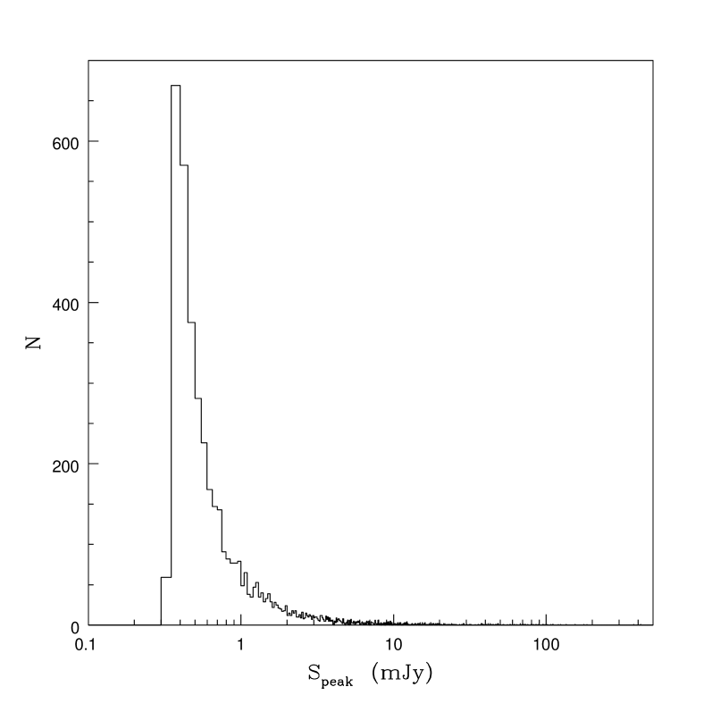
Figure 1: Peak flux density distribution for all the ATESP radio sources (or source components) with $S_{\rm peak}\geq 4.5\sigma$.

2.3 Re-fitting

For the first three groups listed above ad hoc procedures were attempted aimed at improving the fit.
Single-component fits were considered satisfactory whenever positions and flux densities satisfy the tolerance criteria defined above.
In a few cases Gaussian fits were able to provide good values for positions and peak flux densities, but did fail in determining the integrated flux densities. This happens typically at faint fluxes ($<10\sigma$). Gaussian sources with a poor $S_{\rm total}$ value are flagged in the catalogue (see Sect. 3.4).
The islands successfully split in two or three components are 67 in total (64 with two components and 3 with three components).
For non-Gaussian sources we adopted as parameters the reference positions and flux densities defined above. The source position angle was determined by the direction in which the source is most extended and the source axes were defined as largest angular sizes (las), i.e. the maximum distance between two opposite points belonging to the $3\sigma$ flux density contour along (major axis) and perpendicular to (minor axis) the same direction. All the non-Gaussian sources are flagged in the catalogue (see Sect. 3.4).

Figure 2: Local to average noise ratio distribution for all the sources with $S_{\rm peak}\geq 6\sigma_{\rm fit}$. Local noise is defined as the average noise in a $\sim 8\arcmin$ sided box around each source. The distribution is well fitted by a Gaussian with ${\rm FWHM}=0.14$ and peak value equal to 1.01 (solid line). The excess at large $\sigma_{\rm local}/\sigma_{\rm fit}$ values is due to the presence of systematic noise effects (see text).

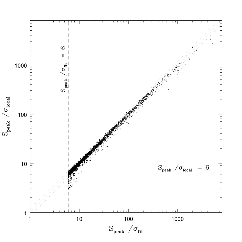
Figure 3: $S_{\rm peak}/\sigma_{\rm local}$ vs. $S_{\rm peak}/\sigma_{\rm fit}$. As expected for random noise distributions, the two signal-to-noise ratios show a tight correlation. Dashed lines indicate the $S_{\rm peak}=6\sigma_{\rm fit}$ (vertical line) and $S_{\rm peak}=6\sigma_{\rm local}$ (horizontal line) cut-off respectively. Also shown are the lines (dotted) between which, under the assumption of a normal noise distribution, one would find 99.9% of the sources.

3 The Source Catalogue

The procedures described in the previous section yielded a preliminary list of sources (or source components) for further investigation. In order to minimize the incompleteness effects present at fluxes approaching the source extraction threshold (see Fig. 1) we decided to insert in the final catalogue only the sources with $S_{\rm peak}\geq 6\sigma$, where $\sigma$ is the mosaic rms flux density. This threshold has been chosen after inspection of the local noise distribution. The local noise ($\sigma_{\rm local}$) has been defined as the average noise value in a box of about $8\arcmin\times 8\arcmin$ size around a source. Usually the local noise does not show significant systematic departures from the mosaic average rms value: the $\sigma_{\rm local}/\sigma_{\rm fit}$ distribution can be described fairly well by a Gaussian with ${\rm FWHM}=0.14$ and peak value equal to 1.01 (see Fig. 2).
This can be seen also in Fig. 3, where we show, for each source, the signal-to-noise ratio defined using both $\sigma_{\rm local}$ and $\sigma_{\rm fit}$. The two signal-to-noise ratios mostly agree with each other, although a number of significant departures are evident for the faintest sources. This is due to the presence of some residual areas where the noise is not random due to systematic effects (noise peaks and stripes). This is caused by the limited dynamical range in presence of very strong sources (stronger than $50-100$ mJy, see also paper I). It is worth noting that also the systematic departures from the expected behavior at the brightest end of the plot ($S_{\rm peak}/\sigma_{\rm local}<S_{\rm peak}/\sigma_{\rm fit}$) are a consequence of the same problem.
In mosaic regions where local noise is significantly larger, we applied a $6\sigma_{\rm local}$ cut-off if $\sigma_{\rm local}/\sigma_{\rm fit}\geq 1.2$ (assuming a normal distribution for the noise, the probability to get a local to average noise value $\geq 1.2$ is $\leq 0.1\%$). This resulted in the rejection of 32 sources (see the region in Fig. 3 defined by $S_{\rm peak}\geq 6\sigma_{\rm fit}$, $S_{\rm peak}<6\sigma_{\rm local}$ and $\sigma_{\rm local}/\sigma_{\rm fit}\geq 1.2$).
The criteria discussed above proved to be very effective in selecting out noise artifacts from the catalogue. Nevertheless a few (6) sources, which satisfy both the average and the local noise constraints are, however, evident noise artifacts at visual inspection. Such objects have been rejected from the final catalogue.
The adopted criteria for the final catalogue definition also allowed us to significantly reduce the number of poor Gaussian fits (see Sect. 2.3) since a large fraction of them ($\sim 65\%$) have fainter $S_{\rm peak}$: we are left with 50 poor Gaussian fits (flagged ‘S*’, see Sect. 3.4) in the final catalogue.
A total number of 3172 source components entered the final catalogue. Some of them have to be considered different components of a unique source and, as discussed later in Sect. 3.2, the number of distinct sources in the ATESP catalogue is 2960.

3.1 Deconvolution

Figure 4: Ratio of the integrated flux $S_{\rm total}$ to the peak one $S_{\rm peak}$ as a function of the source signal-to-noise. Dotted lines indicate the $6\sigma_{\rm fit}$ cut-off adopted for the catalogue definition (vertical line) and the $S_{\rm total}=S_{\rm peak}$ locus (horizontal line) respectively. Also shown are the lower and upper envelopes (dashed lines)of the flux ratio distribution containing $\sim 90\%$ of the unresolved sources (dots). Open circles indicate extended sources.

The ratio of the integrated flux to the peak flux is a direct measure of the extension of a radio source:

$$S_{\rm total}/S_{\rm peak}=\theta_{\rm min}\;\theta_{\rm maj}/b_{\rm min}\;b_{\rm maj}$$ (1)

where $\theta_{\rm min}$ and $\theta_{\rm maj}$ are the source FWHM axes and $b_{\rm min}$ and $b_{\rm maj}$ are the synthesized beam FWHM axes. The flux ratio can therefore be used to discriminate between extended (larger than the beam) and point-like sources.
In Fig. 4 we have plotted the flux ratio as a function of the signal-to-noise for all the sources (or source components) in the ATESP catalogue. The flux density ratio has a skew distribution, with a tail towards high flux ratios due to extended sources. Values for $S_{\rm total}/S_{\rm peak}<1$ are due to the influence of the image noise on the measure of source sizes (see Sect. 4). To establish a criterion for extension, such errors have to be taken into account. We have determined the lower envelope of the flux ratio distribution (the curve containing 90% of the $S_{\rm total}<S_{\rm peak}$ sources) and we have mirrored it on the $S_{\rm total}>S_{\rm peak}$ side (upper envelope in Fig. 4). We have considered as unresolved all sources laying below the upper envelope. The upper envelope can be characterized by the equation:

$$S_{\rm total}/S_{\rm peak}=1.05+\left[\frac{10}{(S_{\rm peak}/\sigma_{\rm fit})^{1.5}}\right]\;.$$ (2)

From this analysis we found that 1864 of the 3172 sources (or source components) in the catalogue (i.e. $\sim 60\%$) have to be considered unresolved.
It is worth noting that the envelope does not converge to 1 going to large signal-to-noise values. This is due to the radial smearing effect. It systematically reduces the source peak fluxes, yielding larger $S_{\rm total}/S_{\rm peak}$ ratios (see discussion in Sect. 4.2). From Fig. 4 we can quantify the smearing effect in $\sim 5\%$ on average.
Deconvolved angular sizes are given in the catalogue only for sources above the upper curve (filled circles in Fig. 4). For unresolved sources (dots in Fig. 4) deconvolved angular sizes are set to zero.
Note that no bandwidth correction to deconvolved sizes has been applied. Correcting for such effect would be somewhat complicated by the fact that each source in the radio mosaics is a sum of contributions from several single pointings.

3.2 Multiple Sources

Figure 5: Nearest neighbor pair density distribution as a function of distance (arcsec) for the ATESP radio sources (histogram) and the expected one assuming a random distribution of the sources in the sky (solid line). The expected distribution has been scaled so as to have the same area below the curve and the observed histogram. The excess at small distances is due to physical associations, and is compensated by a deficiency at intermediate distances (at $d\simeq 80-300\arcsec$). Edge effects explain the discrepancy between the expected distribution and the observed one at very large distances ($d>400\arcsec$). The vertical dashed line indicates the $d=45\arcsec$ cut applied to discriminate between real and unreal physical associations.

Figure 6: Pair components’ flux ratios as a function of the distance between the two components for all the $d\leq 150\arcsec$ pairs in the catalogue. Filled circles indicate solely the pairs that have been considered as part of a unique multiple source in the final form of the catalogue (see text for the criteria adopted for multiple sources’ definition).

In Fig. 5 the (nearest neighbor) pair density distribution is shown as a function of distance (histogram). Also indicated is the expected distribution if all the sample sources (components) were randomly distributed in the sky. The expected distribution has been scaled so as to have the same area below the curve and the observed histogram. The excess at small distances is clearly due to physical associations and, because of the normalization chosen, is compensated by a deficiency at larger distances (between $80\arcsec$ and $300\arcsec$).
All the components closer than $45\arcsec$ (i.e. about three times the beam size) have been considered as possibly belonging to a unique double source. Triple sources are defined whenever one additional component is closer than $45\arcsec$ to (at least) one of the pair components. For multiple sources the same criterion is applied iteratively. Applying this distance constraint we expect that $\sim 20\%$ of the pairs are random superpositions.
The flux ratio distribution between the pair components has a large spread at all distances (see Fig. 6). To reduce the contamination we have discarded all the pairs with flux ratio larger than a factor 10. For triples and multiple sources the probable core is not considered when computing the flux ratios.
A few departures from the adopted criteria are present in the catalogue. For example the triple source ATESP J005620-394145 and the double source ATESP J011029-393253 have $d\leq 45\arcsec$ but do not satisfy the flux ratio constraint. All exceptions are based on source geometry considerations and/or the analysis of the source field.
In order to increase the multiple sources’ sub-sample completeness, we added 31 sources with distances $45\arcsec<d<150\arcsec$, which show clear signs of physical associations between their components (see Fig. 7 for some examples). No flux ratio constraints have been applied to such sources. In Fig. 6 are shown the flux ratios for all the pairs in the final sample of multiple sources (filled circles).
As a final result we have 189 multiple sources: 168 doubles, 19 triples and 2 sources with four components. As a consequence, the initial list of 3172 radio components results in a catalogue of 2960 distinct radio sources.

Table 1: The Radio Catalogue: First Page

IAU Name	R.A.	DEC	$S_{\rm peak}$	$S_{\rm total}$	$\Theta_{\rm maj}$	$\Theta_{\rm min}$	P.A.
	(J2000)		mJy		arcsec		degr.
ATESP J223235-402642	22:32:35.62	-40:26:42.1	1.26	6.07	27.13	13.55	28.9	S
ATESP J223237-393113	22:32:37.71	-39:31:13.2	0.69	0.71	0.00	0.00	0.0	S
ATESP J223238-394102	22:32:38.54	-39:41:02.9	0.48	0.58	0.00	0.00	0.0	S
ATESP J223242-393054	22:32:42.10	-39:30:54.3	2.33	2.46	0.00	0.00	0.0	S
ATESP J223248-401345	22:32:48.24	-40:13:45.9	0.95	0.83	0.00	0.00	0.0	S
ATESP J223250-394059	22:32:50.79	-39:40:59.7	0.57	0.93	10.47	0.00	-88.4	S
ATESP J223252-401925	22:32:52.45	-40:19:25.1	0.66	0.46	0.00	0.00	0.0	S
ATESP J223254-393652	22:32:54.54	-39:36:52.0	1.03	1.70	9.89	5.39	48.3	S
ATESP J223255-395717	22:32:55.51	-39:57:17.3	0.51	0.45	0.00	0.00	0.0	S
ATESP J223256-402010	22:32:56.10	-40:20:10.3	1.13	1.08	0.00	0.00	0.0	S
ATESP J223301-393017	22:33:01.55	-39:30:17.1	7.83	8.67	3.39	2.66	-57.0	S
ATESP J223302-402817	22:33:02.31	-40:28:17.5	0.66	0.71	0.00	0.00	0.0	S
ATESP J223303-401629	22:33:03.07	-40:16:29.2	0.99	1.27	5.30	4.74	62.9	S
ATESP J223304-395639	22:33:04.92	-39:56:39.0	1.85	2.94	23.51	–	–	M
ATESP J223304-395639A	22:33:04.43	-39:56:41.4	1.85	2.18	6.66	1.43	-24.2	S
ATESP J223304-395639B	22:33:06.31	-39:56:32.2	0.80	0.76	0.00	0.00	0.0	S
ATESP J223313-400216	22:33:13.42	-40:02:16.1	7.60	9.18	4.94	3.65	-45.7	S
ATESP J223314-394942	22:33:14.42	-39:49:42.8	1.28	1.33	0.00	0.00	0.0	S
ATESP J223316-393124	22:33:16.90	-39:31:24.4	0.52	0.68	0.00	0.00	0.0	S
ATESP J223317-393235	22:33:17.19	-39:32:35.0	2.40	3.37	9.29	4.22	9.4	S
ATESP J223320-394713	22:33:20.14	-39:47:13.8	0.96	1.08	0.00	0.00	0.0	S
ATESP J223322-401710	22:33:22.93	-40:17:10.7	4.92	6.26	7.56	3.34	14.7	S
ATESP J223327-395836	22:33:27.45	-39:58:36.9	3.24	5.16	13.60	3.39	-5.9	S
ATESP J223327-394541	22:33:27.73	-39:45:41.7	2.74	5.70	21.21	–	–	M
ATESP J223327-394541A	22:33:27.08	-39:45:40.2	2.74	3.65	5.98	4.83	60.7	S
ATESP J223327-394541B	22:33:28.89	-39:45:44.4	1.29	2.05	10.04	0.00	-73.8	S
ATESP J223329-402019	22:33:29.10	-40:20:19.6	1.41	1.82	6.85	3.75	-32.1	S
ATESP J223330-395233	22:33:30.97	-39:52:33.4	0.50	0.53	0.00	0.00	0.0	S
ATESP J223335-401337	22:33:35.21	-40:13:37.7	0.63	0.71	0.00	0.00	0.0	S
ATESP J223337-394253	22:33:37.01	-39:42:53.8	2.58	2.79	0.00	0.00	0.0	S
ATESP J223338-392919	22:33:38.49	-39:29:19.6	5.26	5.62	0.00	0.00	0.0	S
ATESP J223339-393131	22:33:39.86	-39:31:31.0	1.37	1.32	0.00	0.00	0.0	S
ATESP J223343-393811	22:33:43.21	-39:38:11.2	1.00	1.05	0.00	0.00	0.0	S
ATESP J223343-402307	22:33:43.93	-40:23:07.4	0.90	1.10	0.00	0.00	0.0	S
ATESP J223345-402815	22:33:45.23	-40:28:15.6	0.56	0.65	0.00	0.00	0.0	S
ATESP J223346-393322	22:33:46.35	-39:33:22.9	1.26	1.23	0.00	0.00	0.0	S
ATESP J223351-394040	22:33:51.19	-39:40:40.9	1.12	1.17	0.00	0.00	0.0	S
ATESP J223356-401949	22:33:56.57	-40:19:49.7	1.71	2.28	36.37	–	–	M
ATESP J223356-401949A	22:33:55.33	-40:20:11.8	0.52	0.63	0.00	0.00	0.0	S
ATESP J223356-401949B	22:33:57.05	-40:19:41.2	1.71	1.65	0.00	0.00	0.0	S
ATESP J223358-400642	22:33:58.77	-40:06:42.4	1.29	1.20	0.00	0.00	0.0	S
ATESP J223401-402310	22:34:01.25	-40:23:10.8	0.58	1.18	10.98	9.14	32.8	S
ATESP J223401-393448	22:34:01.87	-39:34:48.9	1.69	2.09	5.28	3.10	-72.8	S
ATESP J223402-402357	22:34:02.36	-40:23:57.7	0.59	0.57	0.00	0.00	0.0	S
ATESP J223402-400017	22:34:02.64	-40:00:17.3	1.70	1.99	5.37	2.86	-28.2	S
ATESP J223404-395831	22:34:04.00	-39:58:31.5	6.16	7.45	5.53	3.43	29.7	S
ATESP J223404-393358	22:34:04.08	-39:33:58.9	0.85	0.90	0.00	0.00	0.0	S
ATESP J223407-393721	22:34:07.34	-39:37:21.9	3.14	6.41	25.71	–	–	M
ATESP J223407-393721A	22:34:06.35	-39:37:27.4	2.03	3.23	8.90	6.08	38.9	S
ATESP J223407-393721B	22:34:08.36	-39:37:16.3	3.14	3.19	0.00	0.00	0.0	S
ATESP J223409-394258	22:34:09.58	-39:42:58.2	0.71	1.11	10.16	5.23	-15.4	S
ATESP J223410-394427	22:34:10.82	-39:44:27.6	1.54	1.59	0.00	0.00	0.0	S
ATESP J223412-400254	22:34:12.80	-40:02:54.6	0.66	0.69	0.00	0.00	0.0	S
ATESP J223413-393242	22:34:13.28	-39:32:42.4	1.58	1.88	6.21	0.00	59.9	S
ATESP J223413-393650	22:34:13.74	-39:36:50.2	0.48	1.71	25.27	8.28	38.4	S
ATESP J223413-395651	22:34:13.80	-39:56:51.7	0.52	0.56	0.00	0.00	0.0	S
ATESP J223420-393150	22:34:20.47	-39:31:50.5	0.55	0.73	0.00	0.00	0.0	S

3.3 Non-Gaussian Sources

In the final catalogue we have 23 non-Gaussian sources whose parameters have been defined as discussed in Sect. 2.3. In particular we notice that positions refer to peak positions, which, for non-Gaussian sources does not necessarily correspond to the position of the core. We also notice that we can have non-Gaussian components in multiple sources. Some examples of single and multiple non Gaussian sources are shown in Fig. 7.

Figure 7: Examples of very large ($d>45\arcsec$, see text) multi-component ATESP sources and of non-Gaussian ATESP sources. For direct comparison $4\arcmin\times 4\arcmin$ contour images are presented for all sources. For each source, the contour levels are at 3, 6, 10, 20, 30, 50, 100, 300 times the average rms flux density of the mosaic where the source has been detected. 1^st and 2^nd row: double sources. $3^{rd}$ row: triple sources.

Figure 7: Continued. Examples of very large ($d>45\arcsec$, see text) multi-component ATESP sources and of non-Gaussian ATESP sources. For direct comparison $4\arcmin\times 4\arcmin$ contour images are presented for all sources. For each source, the contour levels are at 3, 6, 10, 20, 30, 50, 100, 300 times the average rms flux density of the mosaic where the source has been detected. 1^st row: the two 4-component sources in the ATESP catalogue. $2^{nd}$ row: single-component non Gaussian sources. $3^{rd}$ row: double sources with one (or two) non-Gaussian components.

3.4 The Catalogue Format

The electronic version of the full radio catalog is available through the ATESP page at http://www.ira.bo.cnr.it. Its first page is shown as an example in Table 1. The source catalogue is sorted on right ascension. The format is the following:

Column (1) - Source IAU name. Different components of multiple sources are labeled ‘A’, ‘B’, etc.
Column (2) and (3) - Source position: Right Ascension and Declination (J2000).
Column (4) and (5) - Source peak ($S_{\rm peak}$) and integrated ($S_{\rm total}$) flux densities in mJy (Baars et al. Baarsetal77 (1977) scale). The flux densities are not corrected for the systematic effects discussed in Sect. 4.2.
Column (6) and (7) - Intrinsic (deconvolved from the beam) source angular size. Full width half maximum of the major ($\Theta_{\rm maj}$) and minor ($\Theta_{\rm min}$) axes in arcsec. Zero values refer to unresolved sources (see Sect. 3.1 for more details).
Column (8) - Source position angle (P.A., measured N through E) for the major axis in degrees.
Column (9) - Flag indicating the fitting procedure and parameterization adopted for the source or source component (see Sects. 2.3 and 3.2). ‘S’ refers to Gaussian fits. ‘S*’ refers to poor Gaussian fits. ‘E’ refers to non-Gaussian sources. ‘M’ refers to multiple sources (see below).

The parameters listed for non-Gaussian sources are defined as discussed in Sect. 2.3.
For multiple sources we list all the components (labeled ‘A’, ‘B’, etc.) preceded by a line (flagged ‘M’) giving the position of the radio centroid, total flux density and overall angular size of the source. Source positions have been defined as the flux-weighted average position of all the components (source centroid). For sources with more than two components the centroid position has been replaced with the core position whenever the core is clearly recognizable.
Integrated total source flux densities are computed by summing all the component integrated fluxes.
The total source angular size is defined as las (see Sect. 2.3) and it is computed as the maximum distance between the source components.

4 Errors in the Source Parameters

Parameter uncertainties are the quadratic sum of two independent terms: the calibration errors, which dominate at high signal-to-noise ratios, and the internal errors, due to the presence of noise in the maps. The latter dominate at low signal-to-noise ratios.
In the following sections we discuss the parameter internal accuracy of our source catalogue. Master equations for total rms error derivation, with estimates of the calibration terms are reported in Appendix A.

4.1 Internal accuracy

In order to quantify the internal errors we produced a one square degree residual map by removing all the sources detected above $5\sigma$ in the radio mosaic fld20to25. We performed a set of Montecarlo simulations by injecting Gaussian sources in the residual map at random positions and re-extracting them using the same detection algorithm used for the survey (IMSAD). The Montecarlo simulations were performed by injecting samples of 30 sources at fixed flux and intrinsic angular size. We sampled peak fluxes between $5\sigma$ and $50\sigma$ and intrinsic angular sizes (FWHM major axis) between $4\arcsec$ and $20\arcsec$. Intrinsic sizes were convolved with the synthesized beam ($8.5\arcsec\times 16.8\arcsec$ for mosaic fld20to25) before injecting the source in the residual map.
The comparison between the input parameters and the ones provided by IMSAD permitted an estimate of the internal accuracy of the parameters as a function of source flux and intrinsic angular size. In particular we could test the accuracy of flux densities, positions and angular sizes and estimate both the efficiency and the accuracy of the deconvolution algorithm.

4.1.1 Flux Densities and Source Sizes

Figure 8: Peak flux density internal accuracy for point sources. Mean and standard deviation for the output/input (IMSAD/injected) ratio, as a function of flux. Expected values (see text) are also plotted for both the mean (dashed line) and the rms (dotted lines). The flux density cut-off chosen for the ATESP catalogue is indicated by the vertical solid line.

Figure 9: Fitted FWHM axes internal accuracy for point sources. Top panel: major axis. Bottom panel: minor axis. Mean and standard deviation for the output/input (IMSAD/injected) ratio, as a function of flux. Expected values (see text) are also plotted for both the mean (dashed line) and the rms (dotted lines). The flux density cut-off chosen for the ATESP catalogue is indicated by the vertical solid line.

The flux density and fitted angular size errors for point sources are shown in in Figs. 8 and 9 where we plot the ratio of the parameter value found by IMSAD (output) over the injected one (input), as a function of the signal-to-noise ratio.
We notice that mean values very far from 1 could indicate the presence of systematic effects in the parameter measure. The presence of such systematic effects is clearly present for peak flux densities in the faintest bins (see Fig. 8). This is the expected effect of the noise on the catalogue completeness at the extraction threshold. Due to its Gaussian distribution whenever an injected source falls on a noise dip, either the source flux is underestimated or the source goes undetected. This produces an incompleteness in the faintest bins. As a consequence, the measured fluxes are biased toward higher values in the incomplete bins, beacause only sources that fall on noise peaks have been detected and measured. We notice that the mean values found for $S_{\rm output}/S_{\rm input}$ are in good agreement with the ones expected taking into account such an effect (see dashed line). It is worth pointing out that our catalogue is only slightly affected by this effect because the detection threshold ($4.5\sigma$) is much lower than the $6\sigma$-threshold chosen for the catalogue (indicated by the vertical solid line in Fig. 8): at $S_{\rm peak}\geq 6\sigma$ we expect flux over-estimations $\leq 5\%$.
Some systematic effects appear to be present also for the source size at $5\sigma$: the major and minor axes tend to be respectively under- and over-estimated (see Fig. 9). Such effects disappear at $S_{\rm peak}\geq 6\sigma$ (ATESP cut-off). For both the flux densities and the source axes, the rms values measured are in very good agreement with the ones proposed by Condon (Condon97 (1997)) for elliptical Gaussian fitting procedures (for details see Appendix A):

$$\sigma(S_{\rm peak})/S_{\rm peak} = 0.93\;\left(\frac{S_{\rm peak}}{\sigma}\right)^{-1}$$ (3)

$$\sigma(\theta_{\rm maj})/\theta_{\rm maj} = 1.24\;\left(\frac{S_{\rm peak}}{\sigma}\right)^{-1}$$ (4)

$$\sigma(\theta_{\rm min})/\theta_{\rm min} = 0.69\;\left(\frac{S_{\rm peak}}{\sigma}\right)^{-1}$$ (5)

where we have applied Eqs. (21) and (41) in Condon (Condon97 (1997)) to the case of ATESP point sources (see dotted lines in Figs. 8 and 9).
The fact that a source is extended does not affect the internal accuracy of the fitting algorithm for both the peak flux density and the source axes. In other words the errors quoted for point sources apply to extended sources as well.
However, this is not true for the deconvolution algorithm. The errors for the deconvolved source axes depend on both the source flux and intrinsic angular size. The higher the flux and the larger the source, the smaller the error. In particular, at 1 mJy ($\sim 12\sigma$) the errors are in the range $35\%$ – $10\%$ for angular sizes in the range $6\arcsec$ – $20\arcsec$. For fluxes $>50\sigma$ the errors are always $<10\%$. Deconvolved angular sizes are unreliable for very faint sources ($5-6\sigma$), where only a very small fraction of sources can be deconvolved. The deconvolution efficiency increases with the source flux. In particular, the fraction of deconvolved sources with intrinsic dimension $\leq 4\arcsec$ never reaches $100\%$: it goes from $3\%$ at the lowest fluxes, to $15\%$ at 1 mJy, to $50\%$ at the highest fluxes. We therefore can assume that $4\arcsec$ is a critical value for deconvolution at the ATESP resolution, and that ATESP sources with intrinsic sizes $\leq 4\arcsec$ are to be considered unresolved.

4.1.2 Source Positions

The positional accuracy for point sources is shown in Fig. 10, where we plot the difference ($\Delta\alpha$ and $\Delta\delta$) between the position found by IMSAD (output) and the injected one (input), as a function of flux. No systematic effects are present and the rms values are in agreement with the ones expected for point sources (Condon Condon98 (1998), for details see Appendix A):

$$\sigma_{\alpha} \simeq \frac{b_{\rm min}}{2}\;\left(\frac{S_{\rm peak}}{\sigma}\right)^{-1}$$ (6)

$$\sigma_{\delta} \simeq \frac{b_{\rm maj}}{2}\;\left(\frac{S_{\rm peak}}{\sigma}\right)^{-1}$$ (7)

where we have assumed $b_{\rm min}=8\arcsec$ and $b_{\rm maj}=14\arcsec$, the average synthesized beam values of the ATESP survey (see dotted lines in Fig. 10). The positional accuracy of ATESP sources is therefore $\sim 1\arcsec$ at the limit of the survey ($6\sigma$), decreasing to $\sim 0.5\arcsec$ at $12\sigma$ ($\sim 1$ mJy) and to $\sim 0.1\arcsec$ at 50$\sigma$.

4.2 Systematic Effects

Figure 10: Position internal accuracy for point sources. Top panel: right ascension. Bottom panel: declination. Mean and standard deviation for the output-input (IMSAD-injected) difference, as a function of flux. Expected values (see text) are also plotted for both the mean (dashed line) and the rms (dotted lines). The flux density cut-off chosen for the ATESP catalogue is indicated by the vertical solid line.

Figure 11: Bandwidth smearing in ATESP single fields calibrated using source ATESP J233758-401025. The measured peak flux density decreases going to larger distances (Top, full circles) while the measured source area increases correspondingly (Bottom, empty circles). As a consequence the integrated flux density remains constant (Top, stars). The curve describing the peak flux density – distance can be used to describe the area – distance relation as well.

Figure 12: Bandwidth smearing in ATESP mosaics. Average $S_{\rm peak}/S_{\rm total}$ ratios obtained by summing all the unresolved ATESP sources brighter than $2$ mJy in different $d_{\rm min}$ intervals (full dots). $d_{\rm min}$ is defined as the distance to the closest field center. Also displayed are radial smearing expected in ATESP single fields (solid line) and in ATESP mosaics (dotted line).

Two systematic effects are to be taken into account when dealing with ATESP flux densities, the clean bias and the bandwidth smearing effect. Clean bias has been extensively discussed in paper I of this series (see also Appendix B at the end of this paper). It is responsible for flux density under-estimations of the order of $10-20\%$ at the lowest flux levels ($S<10\sigma$) and gradually disappears going to higher fluxes (no effect for $S\geq 50-100\sigma$).
The effect of bandwidth smearing is well-known. It reduces the peak flux density of a source, correspondingly increasing the source size in radial direction. Integrated flux densities are therefore not affected.
The bandwidth smearing effect increases with the angular distance ($d$) from the the pointing center of phase and depends on the passband width ($\Delta\nu$), the observing frequency ($\nu$) and the synthesized beam FWHM width ($\theta_{b}$). The particular functional form that describes the bandwidth smearing is determined by the beam and the passband shapes. It can be demonstrated, though, that the results obtained are not critically dependent on the particular functional form adopted (e.g. Bridle & Schwab Bridle89 (1989)).
In the simplest case of Gaussian beam and passband shapes, the bandwidth smearing effect can be described by the equation (see Eq. 12 in Condon et al. Condonetal98 (1998)):

$$\frac{S_{\rm peak}}{S^{0}_{\rm peak}}=\frac{1}{\sqrt{1+\frac{2\ln 2}{3}\left(\frac{\Delta\nu}{\nu}\frac{d}{\theta_{b}}\right)^{2}}}$$ (8)

where the $\frac{S_{\rm peak}}{S^{0}_{\rm peak}}$ ratio represents the attenuation on peak flux densities by respect to the unsmeared ($d=0$) source peak value.
We have estimated the actual smearing radial attenuation on ATESP single fields, by measuring $S_{\rm peak}$ for a strong source (ATESP J233758-401025) detected in eight contiguous ATESP fields (corrected for the primary beam attenuation) at increasing distance from the field center (full circles in Fig. 11, top panel). The data were then fitted using Eq. 8 by setting $\nu=1.4$ GHz and $\theta_{b}\simeq 11\arcsec$ (from ($b_{\rm maj}+b_{\rm min})/2=(14\arcsec+8\arcsec)/2$), as for the ATESP data. The best fit (dashed line in Fig. 11, top panel) gives $S^{0}_{\rm peak}=131$ mJy and an effective bandwidth $\Delta\nu=9$ MHz (in very good agreement with the nominal channel width $\Delta\nu=8$ MHz (see Sect. 5.2 in paper I). As expected, the measured integrated flux density (stars in the same plot) remains constant.
The mosaicing technique consists in a weighted linear combination of all the single fields in a larger mosaiced image (see Eq. 1 in paper I). This means that, given single fields of size $1800\times 1800$ pixels, source flux measures at distances as large as $\simeq 35\arcmin$ from field centers are still used to produce the final mosaic (even if with small weights). As a consequence, the radial dependence of bandwidth smearing tends to cancel out.
For instance, since ATESP pointings are organized in a $20\arcmin$ spacing rectangular grid, a source located at the center of phase of one field ($d=0$) is measured also at $d=20\arcmin$ in the 4 contiguous E, W, S and N fields and at $d=20\cdot\sqrt{2}\simeq 28\arcmin$ in the other 4 diagonally contiguous fields. Using Eq. (1) of paper I, we can estimate a 4% smearing attenuation for the mosaic peak flux of that source. In the same way we can estimate indicative values for mosaic smearing attenuations as a function of $d_{\rm min}$, defined as the distance to the closest field center (see dotted line in Fig. 12). We notice that actual attenuations vary from source to source depending on the actual position of the source in the mosaic.
From Fig. 12 we can see that at small $d_{\rm min}$ mosaic smearing is much worse than single field’s one (indicated by the solid line). The discrepancy becomes smaller going to larger distances and disappears at $d_{\rm min}\simeq 14\arcmin$, which represents the maximum distance to the closest field center for ATESP sources. This maximum $d_{\rm min}$ value gives an upper limit of $\sim 6\%$ to mosaic smearing attenuations.
The expected mosaic attenuations have been compared to the ones obtained directly estimating the smearing from the source catalogue. As already noticed (Sect. 3.1), a ratio $S_{\rm peak}/S_{\rm total}<1$, is purely determined, in case of point sources and in absence of flux measurement errors, by the bandwidth smearing effect, which systematically attenuates the source peak flux, leaving the integrated flux unchanged.
We have then considered all the unresolved ($\Theta_{\rm maj}=0$) ATESP sources with $S_{\rm peak}>2$ mJy and we have plotted the average values of the $S_{\rm peak}/S_{\rm total}$ ratio in different distance intervals (full dots in Fig. 12). The 2 mJy threshold ($\sim 25\sigma$) was chosen in order to find a compromise between statistics and flux measure accuracy. The average flux ratios plotted are in very good agreement with the expected ones, especially when considering that the most reliable measures are the intermediate distance ones, where a larger number of sources can be summed. In general we can conclude that on average smearing attenuations are $\sim 5\%$ and do not depend on the actual position of the source in the mosaics. This result also confirms the $5\%$ estimate drawn from Fig. 4. We finally point out that smearing will affect to some extent also source sizes and source coordinates.

4.3 Comparison with External Data

To determine the quality of ATESP source parameters we have made comparisons with external data. Unfortunately in the region covered by the ATESP, there are not many 1.4 GHz data available. The only existing 1.4 GHz radio survey is the NVSS (Condon et al. Condonetal98 (1998)), which covers about half of the region covered by the ATESP survey ($\delta>-40\degr$) with a point source detection limit $S_{lim}\sim 2.5$ mJy.
The NVSS has a poor spatial resolution ($45\arcsec$ FWHM beam width) compared to ATESP and this introduces large uncertainties in the comparison, especially for astrometry. To test the positional accuracy we have therefore used data at other frequencies as well. In particular we have used VLBI sources extracted from the list of the standard calibrators at the ATCA and the catalogue of PMN compact sources with measured ATCA positions (Wright et al. Wright97 (1997)).

Figure 13: Comparison of NVSS with ATESP flux densities. Dashed lines show the 90% confidence limits in the flux measure.

Figure 14: Result of the cross-identification between ATESP and NVSS catalogues in the overlapping region. Only isolated ATESP sources have been considered (see Sect. 4.3.1). The position offsets ($\Delta\alpha$ and $\Delta\delta$ are expressed in terms of their rms uncertainties ($\sigma_{\alpha}$ and $\sigma_{\delta}$). The $3\sigma$ confidence error circle is also shown.

4.3.1 Flux Densities

In order to estimate the quality of the ATESP flux densities we have compared ATESP with NVSS. To minimize the uncertainties due to the much poorer NVSS resolution we should in principle consider only point-like ATESP sources. Nevertheless, in order to increase the statistics at high fluxes ($S>10$ mJy), we decided to include extended ATESP sources as well. Another source of uncertainty in the comparison is due to the fact that in the NVSS distinct sources closer together than $50\arcsec$ will be only marginally separated. To avoid this problem we have restricted the comparison to bright ($S_{\rm peak}>1$ mJy) isolated ATESP sources: we have discarded all multi-component sources (as defined in Sect. 3.2) and all single-component sources whose nearest neighbor is at a distance $\leq 100\arcsec$ (as in the comparison between the FIRST and the NVSS by White et al. White97 (1997)). We have not used isolated ATESP sources fainter than 1 mJy because we have noticed that there are several cases where NVSS point sources are resolved in two distinct objects in the ATESP images, only one being listed in the ATESP catalogue (i.e. the other one has $S_{\rm peak}<6\sigma$).
In Fig. 13 we have plotted the NVSS against the ATESP flux density for the 443 $S_{\rm peak}>1$ mJy ATESP sources identified (sources within the $3\sigma$ confidence circle in Fig. 14). We have used integrated fluxes for the sources which appear extended at the ATESP resolution (full circles) and peak fluxes for the unresolved ones (dots). Also indicated are the $90\%$ confidence limits (dashed curves), drawn taking into account both the NVSS and the ATESP errors in the flux measure. In drawing the upper line we have also taken into account an average correction for the systematic under-estimation of ATESP fluxes due to clean bias and bandwidth smearing (see Sect. 4.2). The provided NVSS fluxes are already corrected for any systematic effect.
The scatter plot shows that at high fluxes the ATESP flux scale agrees with the NVSS one within a few percents ($\leq 3\%$). This gives an upper limit to calibration errors and/or resolution effects at high fluxes. Going to fainter fluxes the discrepancies between the ATESP and the NVSS fluxes become larger, reaching deviations as high as a factor of 2 at the faintest levels. ATESP fluxes tend to be lower than NVSS fluxes. This could be, at least partly, due to resolution effects. Such effects can be estimated from the comparison between NVSS and ATESP sources itself and from theoretical considerations. Assuming the source integral angular size distribution provided by Windhorst et al. (Windhorst90 (1990)) we have that at the NVSS limit ($S\simeq 2.5$ mJy) about 40% of the sources can be resolved by the ATESP synthesized beam (intrinsic angular sizes $\geq 4\arcsec$). This fraction goes up to $50\%$ at $S\simeq 10$ mJy.
On the other hand, we point out that close to the NVSS catalogue cut-off, incompleteness could affect NVSS fluxes. For instance we have noticed that below 5 mJy, there are several cases where the flux given in the NVSS catalogue is overestimated with respect to the one measured in the NVSS image (even taking into account the applied corrections).

4.3.2 Astrometry

The region covered by the ATESP survey contains two VLBI sources from the ATCA calibrator catalogue: 2227-399 and 0104-408. These sources were not used to calibrate our data and therefore provide an independent check of our ATCA positions. The offset between ATESP and VLBI positions (ATESP–VLBI) for the first and the second source respectively are: $\Delta\alpha=-0.277\arcsec$ and $-0.023\arcsec$; $\Delta\delta=+0.239\arcsec$ and $-0.172\arcsec$. Such offsets indicate that the uncertainty in the astrometry should be within a fraction of arcsec. Obviously, we cannot exclude the presence of systematic effects, but an analysis of the ATESP–NVSS positional offsets gives $\Delta\alpha_{\rm med}=-0.115\arcsec$ and $\Delta\delta_{\rm med}=-0.8\arcsec$ (see Fig. 14).
A more precise comparison could be obtained by using the PMN sources with ATCA position measurements available. Unfortunately the number of such PMN sources in the region covered by the ATESP survey is very small: we found only 12 identifications. Using the 4.8 GHz positions for the PMN sources, we derived (ATESP–ATPMN) $\Delta\alpha_{\rm med}=-0.115\arcsec$ and $\Delta\delta_{\rm med}=-0.3\arcsec$.
We can conclude that all comparisons give consistent results and that the astrometry is accurate within a small fraction of an arcsec. Also systematic offsets, if present, should be very small.

Appendix A Master Equations for Error Derivation

As discussed in Sect. 4, internal errors for the ATESP source parameters are well described by Condon (Condon97 (1997)) equations of error propagation derived for two-dimensional elliptical Gaussian fits in presence of Gaussian noise. In order to get the total rms error on each parameter, a calibration term should be quadratically added. Using Eqs. (21) and (41) in Condon (Condon97 (1997)), total percentage errors for flux densities ($\frac{\sigma(S_{\rm peak})}{S_{\rm peak}}$) and fitted axes ($\frac{\sigma(\theta_{\rm maj})}{\theta_{\rm maj}}$, $\frac{\sigma(\theta_{\rm min})}{\theta_{\rm min}}$) can be calculated from:

$$\sqrt{\frac{2}{\rho^{2}}+\epsilon^{2}}$$ (9)

where $\epsilon$ is the calibration term and the effective signal-to-noise ratio, $\rho$, is given by:

$$\rho^{2}=\frac{\theta_{\rm maj}\theta_{\rm min}}{4\theta_{\rm N}^{2}}\left[1+\left(\frac{\theta_{\rm N}}{\theta_{\rm maj}}\right)^{2}\right]^{\alpha_{\rm M}}\left[1+\left(\frac{\theta_{\rm N}}{\theta_{\rm min}}\right)^{2}\right]^{\alpha_{\rm m}}\frac{S_{\rm peak}^{2}}{\sigma^{2}}$$ (10)

where $\sigma$ is the image noise ($\sim 79$ $\mu$Jy on average for ATESP images), $\theta_{\rm N}$ is the FWHM of the Gaussian correlation length of the image noise (assumed $\simeq$ FWHM of the synthesized beam) and the exponents are:

$$\alpha_{\rm M}=3/2\;\;{\rm and} \alpha_{\rm m}=3/2 {\rm for}\;\;\sigma(S_{\rm peak})$$ (11)

$$\alpha_{\rm M}=5/2\;\;{\rm and} \alpha_{\rm m}=1/2 {\rm for}\;\;\sigma(\theta_{\rm maj})$$ (12)

$$\alpha_{\rm M}=1/2\;\;{\rm and} \alpha_{\rm m}=5/2 {\rm for}\;\;\sigma(\theta_{\rm min})\;.$$ (13)

Similar equations hold for position rms errors (Condon Condon97 (1997), Condon et al. Condonetal98 (1998)):

$$\sigma^{2}(\alpha)= \epsilon^{2}_{\alpha}+\sigma^{2}(x_{0})\sin^{2}({\rm P.A.})+\sigma^{2}(y_{0})\cos^{2}({\rm P.A.})$$ (14)

$$\sigma^{2}(\delta)= \epsilon^{2}_{\delta}+\sigma^{2}(x_{0})\cos^{2}({\rm P.A.})+\sigma^{2}(y_{0})\sin^{2}({\rm P.A.})$$ (15)

where $\sigma^{2}(x_{0})=\sigma^{2}(\theta_{\rm maj})/8\ln 2$ and $\sigma^{2}(y_{0})=\sigma^{2}(\theta_{\rm min})/8\ln 2$ represent the rms lengths of the major and minor axes respectively.
Calibration terms are in general estimated from comparison with consistent external data of better accuracy than the one tested. Unfortunately there are no such data available in the region of sky covered by the ATESP survey. Nevertheless, from our typical flux and phase calibration errors, we estimate calibration terms of about $5-10\%$ for both flux densities and source sizes.
As a caveat we remind (see discussion in Paper I) that the 500 m baseline cutoff applied to our data makes the ATESP survey progressively insensitive to sources larger than $30\arcsec$: assuming a Gaussian shape, only $50\%$ of the flux for a $30\arcsec$ large source would appear in the ATESP images. It is important to have this in mind when dealing with flux densities and source sizes of the largest ATESP sources.
Right ascension and declination calibration terms have been estimated from the astrometry results reported in Sect. 4.3.2. As already discussed, the ATESP astrometry can be considered accurate within a small fraction of an arcsec, even though the scarcity of (accurate) external data available in the ATESP region makes it difficult to quantify this statement. Nevertheless from the rms dispersion of the median offsets found between ATESP and the external comparison samples (see Sect. 4.3.2) we can tentatively estimate $\epsilon_{\alpha}\simeq 0.1\arcsec$ and $\epsilon_{\delta}\simeq 0.4\arcsec$.
It can be easily demonstrated that the master equations (9), (14) and (15) reduce to Eqs. (3) $-$ (7) in Sect. 4 (where the calibration term is neglected) in the case of ATESP point sources ($\theta_{\rm maj}\times\theta_{\rm min}\simeq 14\arcsec\times 8\arcsec$, P.A.$\simeq+2\degr$), assuming $\theta_{\rm N}\simeq 11\arcsec$ (or $\theta_{\rm N}^{2}\sim\theta_{\rm maj}\theta_{\rm min}$).
For a complete and detailed discussion of the error master equations of source parameters obtained through elliptical Gaussian fits we refer to Condon (Condon97 (1997)) and Condon et al. (Condonetal98 (1998)).

Appendix B Flux Density Corrections for Systematic Effects

As already discussed in Sect. 4.2, two systematic effects are to be taken into account when dealing with ATESP flux densities, the clean bias and the bandwidth smearing effect.
The flux densities reported in the ATESP source catalogue are not corrected for such systematic effects. The corrected flux densities ($S^{\rm corr}$) can be computed as follows:

$$S^{\rm corr}=\frac{S^{\rm meas}}{k\cdot[a\log{(S^{\rm corr}/\sigma)}+b]}$$ (16)

where $S^{\rm meas}$ is the flux actually measured in the ATESP images (the one reported in the source catalogue). The parameter $k$ represents the smearing correction. It is set equal to 1 (i.e. no correction) when the equation is applied to integrated flux densities and $<1$ when dealing with peak flux densities. From the analysis reported in Sect. 4.2 we suggest to set $k=0.95$ ($5\%$ smearing effect).
The clean bias correction is taken into account by the term in the square brackets. As discussed in paper I, Sect. 5.3, the importance of the clean bias effect varies from mosaic to mosaic depending on the average number of clean components (cc’s). In particular we derived the values for the parameters $a$ and $b$ in three different mosaics representing the case of low (fld34to40, 1616 cc’s), intermediate (fld44to50, 2377 cc’s) and high (fld69to75, 3119 cc’s) average number of cc’s (see Table 4 of paper I).
In correcting the source fluxes for the clean bias, we suggest to set $(a,b)=(0.09,0.85)$ whenever the mosaic average number of cc’s is $<2000$ (low–cc’s case); $(a,b)=(0.13,0.75)$ whenever the mosaic cc’s average number is between 2000 and 3000 (intermediate–cc’s case); $(a,b)=(0.16,0.67)$ whenever the mosaic cc’s average number exceeds 3000 (high–cc’s case). The average number of clean components for each mosaic is reported in Table 2. In order to trace back the sources to the original mosaics, Table 2 lists also the right ascension range covered by each mosaic (indicated by the r.a. of the first and the last source in that mosaic).
The clean bias is a function of the source signal-to-noise ratio $S^{\rm corr}/\sigma$. Since the noise level is fairly uniform within each mosaic, it is possible to assume $\sigma$ equal to the mosaic average noise value ($\sigma_{fit}$ in Table 2, we refer to paper I for details on mosaic noise analysis and average noise value definition).

Table 2: Mosaic parameters.

Mosaic	cc’s	$\sigma_{fit}$ ($\mu$Jy)	R.A. range
fld01to06	2033	78.7	$22:32:35$ - $22:39:24$
fld05to11	1796	77.8	$22:39:28$ - $22:49:51$
fld10to15	3104	88.1	$22:49:54$ - $22:56:46$
fld20to25	2823	83.0	$23:31:30$ - $23:38:20$
fld24to30	2716	82.8	$23:38:27$ - $23:48:51$
fld29to35	2044	79.2	$23:48:54$ - $23:55:43$
fld34to40	1616	76.3	$23:55:51$ - $00:06:15$
fld39to45	2535	81.2	$00:06:21$ - $00:13:10$
fld44to50	2377	78.0	$00:13:20$ - $00:23:35$
fld49to55	2168	78.6	$00:23:45$ - $00:30:35$
fld54to60	2504	77.3	$00:30:40$ - $00:41:01$
fld59to65	2447	79.4	$00:41:07$ - $00:47:57$
fld64to70	1899	75.1	$00:48:03$ - $00:58:29$
fld69to75	3119	81.9	$00:58:30$ - $01:05:22$
fld74to80	2558	77.1	$01:05:26$ - $01:15:50$
fld79to84	1522	68.9	$01:15:53$ - $01:22:50$

References

- (1) Baars J.W.M., Genzel R., Pauliny-Toth I.I.K., Witzel A., 1977, A&AS 61, 99
- (2) Bridle A.H., Schwab F.R., 1989. In: Perley et al. (eds.) Synthesis Imaging in Radio Astronomy, ASP Conf. Ser. 6, 247
- (3) Condon J.J., 1997, PASP 109, 166
- (4) Condon J.J., 1998. In: B.J. McLean et al. (eds.) Proc. IAU Symp. 179, New Horizons from Multi-Wavelength Sky Surveys, p. 19
- (5) Condon J.J., Cotton W.D., Greiser E.W., et al., 1998, AJ 115, 1693
- (6) Prandoni I., Gregorini L., Parma P., et al., 2000, A&AS 146, 31 (Paper I)
- (7) Sault R.J., Killeen N., 1995, Miriad Users Guide
- (8) Vettolani G., Zucca E., Zamorani G., et al., 1997, A&A 325, 954
- (9) White R.L., Becker R.H., Helfand D.J., Gregg M.D., 1997, ApJ 475, 479
- (10) Windhorst R.A., Mathis D., Neuschaefer L., 1990. In: Kron R.G. (ed.) Evolution of the Universe of Galaxies, ASP Conf. Ser. 10, 389
- (11) Wright A.E., Tasker N., McConnell D., et al., 1997, http://www.parkes.atnf.csiro.au/databases/surveys/