Evolutionary tracks and isochrones for $\alpha$-enhanced stars

Abstract

We present four large sets of evolutionary tracks for stars with initial chemical compositions $[Y=0.250,Z=0.008]$, $[Y=0.273,Z=0.019]$, $[Y=0.320,Z=0.040]$ and $[Y=0.390,Z=0.070]$ and enhancement of $\alpha$ elements with respect to the solar pattern. The major improvement with respect to previous similar calculations is that we use consistent opacities – i.e. computed with the same chemical composition as adopted in the stellar models – over the whole relevant range of temperatures. For the same initial chemical compositions $[Y,Z]$ and otherwise identical input physics we present also new evolutionary sequences with solar-scaled mixtures of abundances. Based on these stellar models we calculate the corresponding sets of isochrones both in the Johnson-Cousins $UBVRIJHK$ and HST/WFPC2 photometric systems. Furthermore, we derive integrated magnitudes, colours and mass-to-light ratios for ideal single stellar populations with total mass equal to $1\,M_{\odot}$. Finally, the major changes in the tracks, isochrones, and integrated magnitudes and colours passing from solar-scaled to $\alpha$-enhanced mixtures are briefly outlined. Retrieval of the complete data set is possible via the www page http://pleiadi.pd.astro.it.

1 Introduction

There are indications both from observations and theoretical studies that stars in many astrophysical environments may have the relative abundances of elements synthesized by nuclear $\alpha$-capture reactions (e.g. C, O, Ne, Mg, Si, Ti, etc) that are enhanced with respect to the solar ones. In brief, King (1994) found the mean [O/Fe] ratio for a handful of halo stars to be $+0.52$ dex. Similar results are found for globular cluster stars (e.g. [$\alpha/{\rm Fe}]=0.18$ dex for 47 Tuc, Carney 1996) and galactic bulge K giants (McWilliam & Rich 1994, Rich & McWilliam 2000). According to models of chemical evolution of the Galaxy, bulge stars should be $\alpha$-enhanced to reproduce the metallicity distribution (Matteucci & Brocato 1990, Matteucci et al. 1999). Indications that the abundance ratios of elements in elliptical galaxies are not solar (e.g. $[{\rm Mg/Fe}]=0.3-0.7$ dex) come from Worthey et al. (1992). Also synthetic metal line strengths (Weiss, Peletier & Matteucci 1995) from high-metallicity models show that solar-scaled models do not fit the observed Mg2 (5180 Å) and Fe (5270 and 5335 Å) line indices.

Given these premises, it is of paramount importance to include the enhancement of $\alpha$-elements in the population synthesis models designed to describe those galaxies. In the past this has been done but using models that suffered from many limitations. Firstly, till recently there were no extended sets of opacities for $\alpha$-enhanced mixtures covering the complete relevant range of stellar temperatures. Such opacity calculations are nowadays available. Secondly, it has often been assumed that the behaviour of $\alpha$-enhanced isochrones can be easily mimicked by suitably scaling the metallicity [Fe/H] (Salaris et al. 1993). However, the validity of such a re-scaling has only been confirmed for low metallicities, and it holds only for some particular cases like all $\alpha$-elements being enhanced by the same factor. Weiss et al. (1995) already pointed out the differences in the evolution due to $\alpha$-enhancement at solar and super-solar metallicities. Recent work by Salaris & Weiss (1998) and VandenBerg et al. (2000) also indicates that the simple re-scaling of the [Fe/H] content becomes risky at high metallicities. Moreover, we should keep in mind that there is no a priori reason, from the point of view of both nucleosynthetic and chemical evolution theories, to expect that all $\alpha$-elements are enhanced by the same factor. From observations of halo and bulge stars, the degree of enhancement of different $\alpha$-elements is, in general, not constant with differences amounting to $\pm 0.2$ dex.

Therefore in this paper we intend to re-analyze the impact of the enhancement of $\alpha$-elements on the properties of metal-rich stellar populations (whose metallicity ranges from half-solar to three times-solar). The analysis is made for a particular choice of $\alpha$-enhanced abundance ratios, for which self-consistent opacities are available. We start calculating extended sets of stellar evolutionary tracks (Sect. 2), with total metal contents $Z=0.008$, 0.019, 0.040 and 0.070 both for solar-scaled (same abundance ratios as in the solar mix) and $\alpha$-enhanced patterns of abundances. Particular attention is paid to the description of the adopted initial element abundances and sources of opacity. Based on those stellar models we derive large grids of isochrones and single stellar populations for which we present magnitudes, colours and mass-to-light ratios in many pass-bands of the Johnson and WFPC2 photometric systems (Sect. 3). Extensive tabulations of stellar models, isochrones and photometric properties are provided in electronic format for the purpose of general use. Finally, a short summary is given in Sect. 4.

VandenBerg et al. (2000) recently presented extensive sets of evolutionary tracks for $\alpha$-enhanced mixtures, limited to the range of low-mass stars ($0.5\leq M/M_{\odot}\leq 1.0$). A constant enhancement of all $\alpha$-elements has been assumed (also in their opacity tables). In the present work, instead, the choice of initial abundances has been guided by observational results. It is worth remarking that, within the present errors, none of both choices seems to be strongly preferred.

2 Stellar tracks

We calculate four grids of stellar models with initial masses from 0.15 to 20 $M_{\odot}$ and initial chemical compositions $[Y=0.250,Z=0.008]$, $[Y=0.273,Z=0.019]$, $[Y=0.320,Z=0.040]$, $[Y=0.390,Z=0.070]$. The metallicities and the helium-to-metal enrichment ratio $\Delta Y/\Delta Z$ are chosen in such a way to secure consistency with the Girardi et al. (2000) models. The helium-to-metal enrichment law is $Y=0.23+2.25\,Z$.

For the above values of $[Y,Z]$, we compute both solar-scaled and $\alpha$-enhanced sets of stellar tracks. The evolutionary phases covered by the grids extend from the zero age main sequence (ZAMS) up to either the start of the thermally pulsing asymptotic giant branch (TP-AGB) phase or carbon ignition.

2.1 Input physics

The input physics of the present stellar models is the same as in Girardi et al. (2000), apart from differences in (i) the opacities, and (ii) the rates of energy loss by plasma neutrinos. A short description of the updated ingredients and the way we deal with the enhancement of $\alpha$-elements is presented in the sections below.

2.1.1 Initial chemical composition

For a fixed total metallicity $Z$, the solar-scaled abundance ratios of metals are taken from Grevesse & Noels (1993). In the $\alpha$-enhanced case, we adopt a mixture in which only the elements resulting from nuclear $\alpha$-capture reactions (O, Ne, Mg, Si, S, Ca, Ti, Ni) are enhanced with respect to the solar abundance ratios. This is the same mixture as used by Salaris et al. (1997) and Salaris & Weiss (1998) to study the age of the oldest metal-poor and disk metal-rich globular clusters. For the sake of clarity, Table 1 lists the abundances for the solar-scaled and $\alpha$-enhanced mixtures. Columns (2) and (4) show the abundance $A_{\rm el}$ of the elements in logarithmic scale, $A_{\rm el}=\log N_{\rm el}/N_{\rm H}+12$, where $N_{\rm el}$ is the abundance by number. Columns (3) and (5) display the abundance by mass fraction $X_{\rm el}$, relative to the metallicity $Z$. Columns (6) and (7) list the enhancement ratio (relative either to Fe or the total metal fraction) in spectroscopic notation. The enhancement factors come from the determinations of chemical abundances in metal-poor field stars by Ryan et al. (1991, cf. also Salaris & Weiss 1998). To derive the initial abundances of different isotopes we use the isotopic ratios (by mass) of Anders & Grevesse (1989).

Table 1: Abundance ratios in the adopted solar-scaled and $\alpha$-enhanced mixtures. See the text for details.

element	solar-scaled		$\alpha$-enhanced
	$A_{\rm el}$	$X_{\rm el}/Z$	$A_{\rm el}$	$X_{\rm el}/Z$	$[A_{\rm el}/{\rm Fe}]$	$[A_{\rm el}/{\rm M}]$
(1)	(2)	(3)	(4)	(5)	(6)	(7)
O	8.870	0.482273	9.370	0.672836	0.50	$+$0.1442
Ne	8.080	0.098668	8.370	0.084869	0.29	$-$0.0658
Mg	7.580	0.037573	7.980	0.041639	0.40	$+$0.0441
Si	7.550	0.040520	7.850	0.035669	0.30	$-$0.0558
S	7.210	0.021142	7.540	0.019942	0.33	$-$0.0258
Ca	6.360	0.003734	6.860	0.005209	0.50	$+$0.1441
Ti	5.020	0.000211	5.650	0.000387	0.63	$-$0.1875
Ni	6.250	0.004459	6.270	0.002056	0.02	$-$0.3371
C	8.550	0.173285	8.550	0.076451	0.00	$-$0.3553
N	7.970	0.053152	7.970	0.023450	0.00	$-$0.3553
Na	6.330	0.001999	6.330	0.000882	0.00	$-$0.3553
Cr	5.670	0.001005	5.670	0.000443	0.00	$-$0.3557
Fe	7.500	0.071794	7.500	0.031675	0.00	$-$0.3557

2.1.2 Opacities

The opacities we have adopted are the same as in Salaris, Degl’Innocenti & Weiss (1997). They are available at: http://www-phys.llnl.gov/V_Div/OPAL/existing.html. Details are given below.

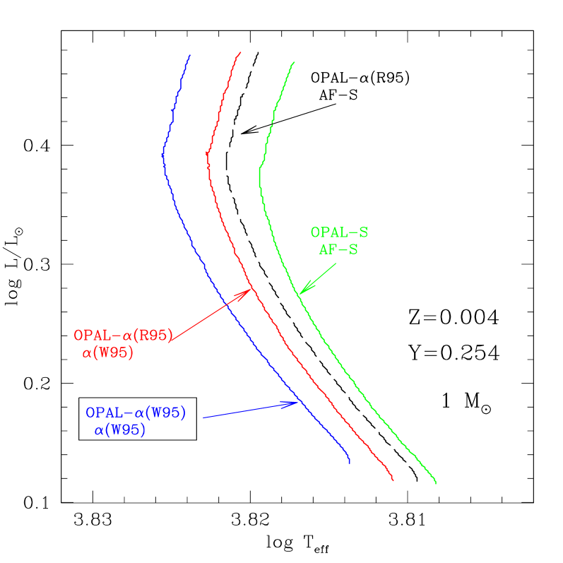
Figure 1: Evolution of a 1 $M_{\odot}$ star with the indicated chemical composition up to the age of the Sun according to different opacity sources and enhancements of $\alpha$-elements. See text for the meaning of the various labels and more details.

For high temperatures ($\log T\geq 4$) we use the radiative OPAL opacities by Rogers & Iglesias (1995) in the case of solar-scaled mixtures, and by Iglesias & Rogers (1996) for the $\alpha$-enhanced ones. At low temperatures these are combined with the molecular opacities provided by Alexander & Ferguson (1994) for the solar mixtures, and by Alexander (priv. communication) for the $\alpha$-enhanced ones. In both cases, low- and high-temperature opacity grids are merged by interpolation in the temperature range from $\log T=3.8$ to $\log T=4$. For very high temperatures, $\log T\geq 8.7$, the Weiss et al. (1990) opacities are used. These rely on the Los Alamos opacity database. The radiative opacities for C, O mixtures, needed in the post-main sequence phases, are from Iglesias & Rogers (1993). Finally, conductive opacities of electron-degenerate matter are from Itoh et al. (1983).

It is very important to emphasize that the present models are based on complete and consistent opacities, i.e.  the opacities (both for solar and $\alpha$-enhanced mixtures) are generated for the same pattern of abundances adopted in the stellar models, both at low and high temperatures.

The importance of this issue is illustrated by Fig. 1, which shows the effect in the Hertzsprung-Russell (HR) diagram of adopting different (inconsistent) opacities and/or mixtures and/or enhancement factors as input to a 1 $M_{\odot}$ main sequence model with $[Z=0.004,Y=0.254]$. Some of the illustrated cases are often found in literature. The tracks are evolved up to the solar age of 4.6 Gyr. The meaning of the labels is the following: the first label refers to high temperature opacity ($\log T>4$) and can vary from OPAL-S, i.e. solar-scaled mixture, to OPAL-$\alpha$, i.e. enhanced according to Salaris & Weiss (1998; W95) or Rogers (priv. communication; R95). This latter case is a special $\alpha$-enhanced mixture characterized, if compared with Salaris & Weiss (1998), by more C, less O, more Ne, more Na (which is not an alpha-element), less Al, more S, and more Fe. The second label refers to the molecular opacity, with the same notation as for solar and $\alpha$-enhanced mixtures. AF stands for Alexander & Ferguson (1994). The prescription enclosed in a box represents the one adopted by us.

Another point to emphasize is the difference between the present opacities and those used by Girardi et al. (2000). Two are the main sources of differences. First the adoption of the Itoh et al. (1983) conductive opacities instead of the older ones by Hubbard & Lampe (1969). Interestingly, Catelan et al. (1996) show that Itoh et al. (1983) conductive opacities should not be used in RGB models, because they are valid only for a liquid phase, and not for the physical conditions existing in the interiors of RGB stars. However, we verified that the effect of using the Itoh et al. (1983) opacities instead of the Hubbard & Lampe (1969) is to increase the core mass at the helium flash by 0.006 $M_{\odot}$ (see also Castellani et al. 2000 and Cassisi et al. 1998), which is a negligible effect.

The second difference lies in the numerical technique used to interpolate within the grids of the opacity tables. In this paper we use the two-dimensional bi-rational cubic damped-spline algorithm (see Schlattl & Weiss 1998; and Späth 1973), whereas Girardi et al. (2000) adopted the smooth bi-parabolic spline interpolation (SSI) already introduced in our code by Bressan et al. (1993). We verified that the differences amount to about a few percent.

In general, evolutionary models of low mass differ very little by changing the opacity interpolation scheme. However, massive stars (say $M\geq 5M_{\odot}$) are much more sensitive to the interpolation algorithm. This is shown in Fig. 2, where we plot two 4 $M_{\odot}$ and 6 $M_{\odot}$ models with $[Z=0.008,Y=0.250]$ calculated both with the SSI (continuous lines) and the damped-spline (dashed lines) scheme.

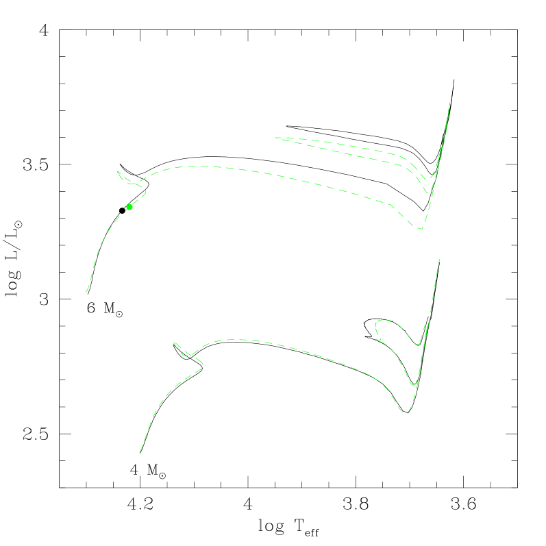
Figure 2: Evolution of the 4 and 6 $M_{\odot}$ models according to different opacity interpolation schemes. The dashed lines are tracks calculated with the damped spline, whereas the continuous lines are tracks calculated with SSI spline. The dots indicate the points when the central hydrogen mass fraction is $X_{\rm c}=0.2$. See also the companion Fig. 3 for more details on the opacity.

Figure 3 compares the effects of the different interpolations on the opacity at the physical conditions holding in the inner regions of a 6 $M_{\odot}$ star when the central hydrogen mass fraction is $X_{\rm c}=0.2$, i.e. at the stage marked with a dot in Fig. 2. At this stage the temperature at the Schwarzschild border of the convective core is $\log T=7.38$ and the density is $\log\rho=1.05$ (corresponding to the arrow in the Fig. 3). For the temperatures indicated along the curves, these represent the opacity as a function of the quantity $\log R=\log\rho-3\log T+18$ (see Rogers & Iglesias 1992 for more details). The continuous curve is based on the SSI interpolation, whereas the dashed curve refers to the method adopted in the present study. The small difference in opacity at the core border is typical of the values found throughout the evolutionary sequences, and is responsible for the different HR patterns.

We notice that both interpolations are acceptable, because the percentage error associated to both of them is roughly 3 %, which is lower than the opacity uncertainty in the original OPAL tables (the latter can be as high as 10 % at individual $T/\rho$ points). This shows that even the fine OPAL grid for some applications is not sufficiently dense and more grid points might be needed. This is also illustrated by the Solar Model by Schlattl & Weiss (1998), where the inverse situation, i.e. spline producing a nicer opacity run, is found.

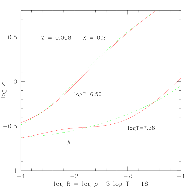
Figure 3: The opacity $\kappa$ as a function of the density and temperature as indicated. The dashed lines are for damped-splined opacity interpolations, the continuous lines are for the bi-parabolic splined ones. The arrow shows the location of the Schwarzschild border of the convective core in a 6 $M_{\odot}$ model with initial chemical composition $[Z=0.008,Y=0.250]$ during the main sequence phase, when the central hydrogen mass fraction is $X_{\rm c}=0.2$. For this model the temperature at the core border is $\log T=7.38$.

The reason for the different luminosities in the high-mass models, is that in these stars the radiative gradient across the border of the convective core is shallow. Therefore, even slightly larger opacities at the Schwarzschild border may cause an increase of the convective core and lead to higher luminosities. This trend already begins during the core H-burning phase and remains during the subsequent evolution. The effects are detectable starting from stars with mass larger than $6-10$ $M_{\odot}$ (see Fig. 2) and becomes dramatic over 60 $M_{\odot}$. It is worth recalling that the maximum mass of our stellar models is 20 $M_{\odot}$.

2.1.3 Neutrino losses

Energy losses by neutrinos are from Haft et al. (1994). Compared with the previous ones of Munakata et al. (1985) used by Girardi et al. (2000), neutrino cooling during the RGB is more efficient. This causes an increase of 0.005 $M_{\odot}$ in the core mass at helium ignition. We have checked this on a 1 $M_{\odot}$ model with $Z=0.019$. Differences of the same order have been found by other authors (e.g. Haft et al. 1994; Cassisi et al. 1998).

2.1.4 Remaining physical input

The remaining physical input is the same as in Girardi et al. (2000), to whom we refer for further details. In summary, we follow the evolution of H, ³He, ⁴He, ¹²C, ¹³C, ¹⁴N, ¹⁵N, ¹⁶O, ¹⁷O, ¹⁸O, ²⁰Ne, ²²Ne, Mg, according to the nuclear reaction rates of Caughlan & Fowler (1988) and Landré et al. (1990). For Mg we refer to the total content of ²⁴Mg, ²⁵Mg and ²⁶Mg.

Figure 4: Evolutionary tracks for the composition $[Y=0.250,Z=0.008]$ and the $\alpha$-enhanced mixture of abundances. The initial mass in solar units is indicated along each curve.

Figure 5: Evolutionary tracks (same composition as Fig. 4) for low-mass models up to the RGB-tip.

Figure 6: Evolutionary tracks (same composition as Fig. 4) for low-mass models from the ZAHB to the start of the TP-AGB phase.

The equation of state (EOS) is that of a fully-ionized gas for temperatures higher that $10^{7}$ K. For lower temperatures we adopt the Mihalas et al. (1990 and references therein) EOS.

Calibration of the solar model fixes the value of the mixing length parameter $\alpha$ of the Böhm-Vitense (1958) theory at 1.68. Overshooting both from the convective core and the convective envelope are taken into account according to the ballistic algorithm by Bressan et al. (1981). Table 2 summarizes the values of the overshooting parameters for the core, $\Lambda_{\rm c}$, and envelope, $\Lambda_{\rm e}$ we have adopted as a function of the initial mass.

As far as the mass-loss is concerned, this is taken into account and its effect on the stellar structure is calculated for masses higher than 6 $M_{\odot}$. We used the same prescription adopted by Fagotto et al. (1994), where more details can be found.

Table 2: Adopted parameters in the overshooting model by Bressan et al. (1981) and Alongi et al. (1991), as a function of the initial mass $M$ (in $M_{\odot}$).

$M/M_{\odot}$	$\Lambda_{\rm c}$	$\Lambda_{\rm e}$
0.5 - 1.0	0	0.25
1.1 - 1.4	$M-1$	0.25
1.5 - 2.0	0.5	0.25
2.0 - 2.5	0.5	$0.5(2.5-M)+1.4(M-2)$
2.5 - 20	0.5	0.7

2.2 HR diagram

For the sake of illustration, in Figs. 4, 5 and 6 we present the complete set of evolutionary tracks for $[Y=0.250,Z=0.008]$ and $\alpha$-enhanced mixtures.

Fig. 4 shows the models of intermediate-mass stars from the zero age main sequence (ZAMS) up to the TP-AGB phase and those of massive stars from the ZAMS up to carbon ignition. Fig. 5 presents the low-mass tracks from the ZAMS up to the RGB-tip. Finally, Fig. 6 shows the corresponding He-burning phase from the zero age horizontal branch (ZAHB) up to the TP-AGB phase.

Some relevant physical quantities are given in Table 3, which lists, as a function of the initial mass, the lifetimes in years of the central H-burning and He-burning phases, $t_{\rm H}$ and $t_{\rm He}$ respectively, the core mass at the helium ignition, $M_{\rm c}({\rm HeF})$, and the core mass at the first thermal pulse on the AGB phase, $M_{\rm c}({\rm 1^{st}-TP})$. For intermediate-mass and massive stars, $M_{\rm c}({\rm HeF})$ refers to the core mass at the He-ignition. For the same chemical composition Table 4 reports the changes in the surface chemical abundances of those elements that suffered from nuclear processing via the pp-chain and CNO-cycle in the deep interiors, after the completion of the first and the second dredge-up by envelope mixing. The surface abundances of heavier elements are not altered by nuclear processing. The last two columns give the ratios of ¹⁴N and ¹⁶O with respect to their initial values. These ratios are indicative of the efficiency of the dredge-up episodes.

Figure 7: Core mass at He ignition as a function of the initial mass, for both solar-scaled (upper panel) and $\alpha$-enhanced  (bottom panel) models.

Table 5 displays the transition masses $M_{\rm conv}$, $M_{\rm HeF}$ and $M_{\rm up}$ for models calculated with solar and $\alpha$-enhanced initial composition. In brief, $M_{\rm conv}$ is the maximum mass below which stars become fully convective during the central H-burning phase, $M_{\rm HeF}$ is the maximum mass for the core He-flash to occur, and finally $M_{\rm up}$ is the maximum mass for the central C-burning to occur in highly electron degenerate gas (deflagration or detonation followed by disruption of the star).

Table 3: Lifetimes of the central H-burning $t_{\rm H}$ and He-burning $t_{\rm He}$ phases, the core mass at the helium ignition $M_{\rm c}({\rm HeF})$ and the core mass $M_{\rm c}(\mbox{1-TP})$ at first thermal pulse on AGB phase, for the models with $Z=0.008$ and solar-scaled mixture (columns 2 to 5) and for the models with $Z=0.07$ and $\alpha$-enhanced mixture (columns 6 to 9).

	$Z=0.008$ solar-scaled				$Z=0.07$ $\alpha$-enhanced
$M/M_{\odot}$	$t_{\rm H}/$yr	$t_{\rm He}/$yr	$M_{\rm c}({\rm HeF})$	$M_{\rm c}(\rm{1^{st}-TP})$	$t_{\rm H}/$yr	$t_{\rm He}/$yr	$M_{\rm c}({\rm HeF})$	$M_{\rm c}(\rm{1^{st}-TP})$
0.6	5.45 $10^{10}$	1.05 $10^{8}$	0.4814	0.5108	4.48 $10^{10}$	1.08 $10^{8}$	0.4445	0.5398
0.7	3.14 $10^{10}$	1.04 $10^{8}$	0.4806	0.5159	2.45 $10^{10}$	1.05 $10^{8}$	0.4434	0.5614
0.8	1.87 $10^{10}$	1.03 $10^{8}$	0.4793	0.5192	1.42 $10^{10}$	1.02 $10^{8}$	0.4434	0.5756
0.9	1.18 $10^{10}$	1.02 $10^{8}$	0.4781	0.5258	8.28 $10^{9}$	1.01 $10^{8}$	0.4430	0.5926
1.0	7.64 $10^{9}$	1.02 $10^{8}$	0.4782	0.5272	5.11 $10^{9}$	1.01 $10^{8}$	0.4426	0.5769
1.1	5.26 $10^{9}$	1.01 $10^{8}$	0.4776	0.5317	3.64 $10^{9}$	9.92 $10^{7}$	0.4424	0.6049
1.2	3.90 $10^{9}$	1.00 $10^{8}$	0.4778	0.5312	2.89 $10^{9}$	9.87 $10^{7}$	0.4418	0.6079
1.3	3.19 $10^{9}$	9.83 $10^{7}$	0.4778	0.5291	2.39 $10^{9}$	9.71 $10^{7}$	0.4421	0.6049
1.4	2.68 $10^{9}$	9.79 $10^{7}$	0.4763	0.5314	2.01 $10^{9}$	9.89 $10^{7}$	0.4375	0.6064
1.5	2.28 $10^{9}$	1.07 $10^{8}$	0.4642	0.5273	1.71 $10^{9}$	1.11 $10^{8}$	0.4169	0.6022
1.6	1.87 $10^{9}$	1.14 $10^{8}$	0.4539	0.5245	1.40 $10^{9}$	1.23 $10^{8}$	0.3999	0.5947
1.7	1.57 $10^{9}$	1.26 $10^{8}$	0.4391	0.5194	1.16 $10^{9}$	1.36 $10^{8}$	0.3845	0.5875
1.8	1.33 $10^{9}$	1.44 $10^{8}$	0.4192	0.5065	9.76 $10^{8}$	1.46 $10^{8}$	0.3680	0.5913
1.9	1.15 $10^{9}$	3.10 $10^{8}$	0.3337	0.4893	8.28 $10^{8}$	1.70 $10^{8}$	0.3406	0.5849
2.0	9.90 $10^{8}$	2.71 $10^{8}$	0.3451	0.4909	7.11 $10^{8}$	2.15 $10^{8}$	0.3281	0.5730
2.2	7.65 $10^{8}$	2.10 $10^{8}$	0.3757	0.5104	5.33 $10^{8}$	1.71 $10^{8}$	0.3598	0.6114
2.5	5.44 $10^{8}$	1.44 $10^{8}$	0.4246	0.5452	3.66 $10^{8}$	1.21 $10^{8}$	0.4104	0.6117
3.0	3.39 $10^{8}$	7.36 $10^{7}$	0.5367	0.6483	2.16 $10^{8}$	6.60 $10^{7}$	0.5178	0.6844
3.5	2.31 $10^{8}$	3.98 $10^{7}$	0.6718	0.7806	1.40 $10^{8}$	3.77 $10^{7}$	0.6408	0.6844
4.0	1.67 $10^{8}$	2.48 $10^{7}$	0.8213	0.9375	9.71 $10^{7}$	2.34 $10^{7}$	0.7713	0.6844
4.5	1.27 $10^{8}$	1.67 $10^{7}$	0.9744	1.0910	7.12 $10^{7}$	1.56 $10^{7}$	0.9092	0.6844
5.0	1.00 $10^{8}$	1.21 $10^{7}$	1.1333	1.2497	5.45 $10^{7}$	1.10 $10^{7}$	1.0593	1.2062
6.0	6.72 $10^{7}$	6.73 $10^{6}$	1.4456	-	3.53 $10^{7}$	6.06 $10^{6}$	1.3904	1.5452
7.0	4.87 $10^{7}$	4.55 $10^{6}$	1.7673	-	2.51 $10^{7}$	3.89 $10^{6}$	1.7609	-
8.0	3.76 $10^{7}$	3.30 $10^{6}$	2.1265	-	1.91 $10^{7}$	2.74 $10^{6}$	2.1599	-
9.0	3.03 $10^{7}$	2.52 $10^{6}$	2.4985	-	1.53 $10^{7}$	2.06 $10^{6}$	2.5988	-
10.0	2.51 $10^{7}$	2.02 $10^{6}$	2.9138	-	1.28 $10^{7}$	1.62 $10^{6}$	3.0935	-
12.0	1.86 $10^{7}$	1.43 $10^{6}$	3.7804	-	9.59 $10^{6}$	1.14 $10^{6}$	3.9767	-
15.0	1.34 $10^{7}$	1.03 $10^{6}$	4.6706	-	7.10 $10^{6}$	8.26 $10^{5}$	5.3587	-
20.0	9.39 $10^{6}$	7.12 $10^{5}$	6.7187	-	5.17 $10^{6}$	6.01 $10^{5}$	7.7582	-

$M_{\rm HeF}$ is here defined as the initial mass for which the core mass at He ignition has its minimum value (see Table 3 and Fig. 7). Fig. 7 shows that similar values for $M_{\rm HeF}$ are found both in the $\alpha$-enhanced and in the solar-scaled case. Compared with Girardi et al. (2000), we find higher $M_{\rm up}$ values. This is once more caused by the different interpolation schemes of the opacity tables. The one currently in use yields smaller convective cores for the same initial mass. It follows that with the present overshooting prescription the maximum mass for a star to develop an electron-degenerate core after the core He-burning phase is slightly higher than previously estimated.

Table 4: Surface chemical composition (by mass fraction) of the $[Z=0.008,Y=0.250]$ solar-scaled models.

$M/M_{\odot}$

H

3He

4He

12C

13C

14N

15N

16O

17O

18O

$\frac{{}^{12}{\rm C}}{{}^{12}{\rm C}_{\rm i}}$

$\frac{{}^{14}{\rm N}}{{}^{14}{\rm N}_{\rm i}}$

Initial:

all

0.742

3.80$\,10^{-5}$

0.250

1.37$\,10^{-3}$

1.65$\,10^{-5}$

4.24$\,10^{-4}$

1.67$\,10^{-6}$

3.85$\,10^{-3}$

1.56$\,10^{-6}$

8.68$\,10^{-6}$

1.00

1.00

After the first dredge-up:

0.60

0.730

3.95$\,10^{-3}$

0.258

1.37$\,10^{-3}$

1.72$\,10^{-5}$

4.24$\,10^{-4}$

1.66$\,10^{-6}$

3.85$\,10^{-3}$

1.56$\,10^{-6}$

8.68$\,10^{-6}$

1.00

1.00

0.70

0.727

2.73$\,10^{-3}$

0.263

1.36$\,10^{-3}$

2.50$\,10^{-5}$

4.26$\,10^{-4}$

1.55$\,10^{-6}$

3.85$\,10^{-3}$

1.56$\,10^{-6}$

8.68$\,10^{-6}$

0.993

1.01

0.80

0.725

1.97$\,10^{-3}$

0.265

1.32$\,10^{-3}$

3.71$\,10^{-5}$

4.59$\,10^{-4}$

1.44$\,10^{-6}$

3.85$\,10^{-3}$

1.56$\,10^{-6}$

8.64$\,10^{-6}$

0.964

1.08

0.90

0.724

1.55$\,10^{-3}$

0.267

1.27$\,10^{-3}$

4.02$\,10^{-5}$

5.18$\,10^{-4}$

1.36$\,10^{-6}$

3.85$\,10^{-3}$

1.57$\,10^{-6}$

8.52$\,10^{-6}$

0.925

1.22

1.00

0.723

1.20$\,10^{-3}$

0.267

1.22$\,10^{-3}$

4.13$\,10^{-5}$

5.72$\,10^{-4}$

1.30$\,10^{-6}$

3.85$\,10^{-3}$

1.60$\,10^{-6}$

8.30$\,10^{-6}$

0.891

1.35

1.10

0.723

1.01$\,10^{-3}$

0.268

1.17$\,10^{-3}$

4.24$\,10^{-5}$

6.35$\,10^{-4}$

1.22$\,10^{-6}$

3.85$\,10^{-3}$

1.70$\,10^{-6}$

8.04$\,10^{-6}$

0.851

1.50

1.20

0.725

8.67$\,10^{-4}$

0.267

1.14$\,10^{-3}$

4.38$\,10^{-5}$

6.70$\,10^{-4}$

1.18$\,10^{-6}$

3.85$\,10^{-3}$

1.83$\,10^{-6}$

7.89$\,10^{-6}$

0.829

1.58

1.30

0.726

8.00$\,10^{-4}$

0.265

1.11$\,10^{-3}$

4.18$\,10^{-5}$

7.00$\,10^{-4}$

1.15$\,10^{-6}$

3.85$\,10^{-3}$

2.01$\,10^{-6}$

7.72$\,10^{-6}$

0.811

1.65

1.40

0.724

6.89$\,10^{-4}$

0.268

1.02$\,10^{-3}$

4.59$\,10^{-5}$

8.06$\,10^{-4}$

1.02$\,10^{-6}$

3.85$\,10^{-3}$

2.56$\,10^{-6}$

7.28$\,10^{-6}$

0.742

1.90

1.50

0.723

6.11$\,10^{-4}$

0.268

9.81$\,10^{-4}$

4.49$\,10^{-5}$

8.53$\,10^{-4}$

9.72$\,10^{-7}$

3.84$\,10^{-3}$

1.02$\,10^{-5}$

7.02$\,10^{-6}$

0.716

2.01

1.60

0.724

5.35$\,10^{-4}$

0.268

9.56$\,10^{-4}$

4.47$\,10^{-5}$

9.02$\,10^{-4}$

9.44$\,10^{-7}$

3.82$\,10^{-3}$

1.02$\,10^{-5}$

6.86$\,10^{-6}$

0.697

2.13

1.70

0.722

4.76$\,10^{-4}$

0.269

9.34$\,10^{-4}$

4.50$\,10^{-5}$

9.66$\,10^{-4}$

9.15$\,10^{-7}$

3.77$\,10^{-3}$

1.70$\,10^{-5}$

6.76$\,10^{-6}$

0.681

2.28

1.80

0.720

4.21$\,10^{-4}$

0.272

9.04$\,10^{-4}$

4.39$\,10^{-5}$

1.04$\,10^{-3}$

8.88$\,10^{-7}$

3.72$\,10^{-3}$

1.93$\,10^{-5}$

6.60$\,10^{-6}$

0.660

2.46

1.90

0.718

3.78$\,10^{-4}$

0.274

9.01$\,10^{-4}$

4.45$\,10^{-5}$

1.09$\,10^{-3}$

8.76$\,10^{-7}$

3.67$\,10^{-3}$

1.63$\,10^{-5}$

6.55$\,10^{-6}$

0.658

2.57

2.00

0.718

3.38$\,10^{-4}$

0.274

8.95$\,10^{-4}$

4.41$\,10^{-5}$

1.12$\,10^{-3}$

8.72$\,10^{-7}$

3.64$\,10^{-3}$

1.63$\,10^{-5}$

6.52$\,10^{-6}$

0.653

2.65

2.20

0.714

2.76$\,10^{-4}$

0.278

8.88$\,10^{-4}$

4.51$\,10^{-5}$

1.20$\,10^{-3}$

8.57$\,10^{-7}$

3.57$\,10^{-3}$

1.53$\,10^{-5}$

6.45$\,10^{-6}$

0.648

2.82

2.50

0.711

2.13$\,10^{-4}$

0.280

8.72$\,10^{-4}$

4.53$\,10^{-5}$

1.27$\,10^{-3}$

8.37$\,10^{-7}$

3.51$\,10^{-3}$

1.16$\,10^{-5}$

6.36$\,10^{-6}$

0.636

3.00

3.00

0.713

1.50$\,10^{-4}$

0.279

8.65$\,10^{-4}$

4.47$\,10^{-5}$

1.30$\,10^{-3}$

8.27$\,10^{-7}$

3.48$\,10^{-3}$

9.83$\,10^{-6}$

6.30$\,10^{-6}$

0.631

3.08

3.50

0.717

1.13$\,10^{-4}$

0.275

8.78$\,10^{-4}$

4.66$\,10^{-5}$

1.27$\,10^{-3}$

8.23$\,10^{-7}$

3.50$\,10^{-3}$

6.74$\,10^{-6}$

6.42$\,10^{-6}$

0.641

2.99

4.00

0.718

9.02$\,10^{-5}$

0.274

8.80$\,10^{-4}$

4.83$\,10^{-5}$

1.27$\,10^{-3}$

8.10$\,10^{-7}$

3.50$\,10^{-3}$

5.56$\,10^{-6}$

6.43$\,10^{-6}$

0.642

2.99

4.50

0.720

7.69$\,10^{-5}$

0.272

9.13$\,10^{-4}$

4.77$\,10^{-5}$

1.22$\,10^{-3}$

8.49$\,10^{-7}$

3.51$\,10^{-3}$

3.89$\,10^{-6}$

6.64$\,10^{-6}$

0.666

2.89

5.00

0.721

6.49$\,10^{-5}$

0.270

9.49$\,10^{-4}$

4.64$\,10^{-5}$

1.18$\,10^{-3}$

8.90$\,10^{-7}$

3.51$\,10^{-3}$

3.70$\,10^{-6}$

6.73$\,10^{-6}$

0.693

2.79

6.00

0.722

4.75$\,10^{-5}$

0.270

8.75$\,10^{-4}$

4.96$\,10^{-5}$

1.28$\,10^{-3}$

7.79$\,10^{-7}$

3.50$\,10^{-3}$

4.04$\,10^{-6}$

6.40$\,10^{-6}$

0.638

3.01

7.00

0.723

3.85$\,10^{-5}$

0.269

8.55$\,10^{-4}$

5.00$\,10^{-5}$

1.32$\,10^{-3}$

7.51$\,10^{-7}$

3.47$\,10^{-3}$

3.84$\,10^{-6}$

6.28$\,10^{-6}$

0.624

3.12

8.00

0.721

3.26$\,10^{-5}$

0.271

8.41$\,10^{-4}$

4.98$\,10^{-5}$

1.37$\,10^{-3}$

7.31$\,10^{-7}$

3.43$\,10^{-3}$

3.61$\,10^{-6}$

6.15$\,10^{-6}$

0.614

3.24

9.00

0.722

3.06$\,10^{-5}$

0.270

8.83$\,10^{-4}$

4.99$\,10^{-5}$

1.31$\,10^{-3}$

7.83$\,10^{-7}$

3.45$\,10^{-3}$

2.77$\,10^{-6}$

6.42$\,10^{-6}$

0.644

3.08

10.00

0.721

2.78$\,10^{-5}$

0.271

8.79$\,10^{-4}$

4.92$\,10^{-5}$

1.33$\,10^{-3}$

7.79$\,10^{-7}$

3.43$\,10^{-3}$

2.83$\,10^{-6}$

6.37$\,10^{-6}$

0.641

3.13

12.00

0.713

2.36$\,10^{-5}$

0.279

8.62$\,10^{-4}$

5.03$\,10^{-5}$

1.44$\,10^{-3}$

7.52$\,10^{-7}$

3.33$\,10^{-3}$

2.49$\,10^{-6}$

6.21$\,10^{-6}$

0.629

3.40

15.00

0.687

1.90$\,10^{-5}$

0.305

8.23$\,10^{-4}$

4.94$\,10^{-5}$

1.67$\,10^{-3}$

7.15$\,10^{-7}$

3.12$\,10^{-3}$

2.24$\,10^{-6}$

5.81$\,10^{-6}$

0.601

3.94

After the second dredge-up:

4.00

0.694

8.64$\,10^{-5}$

0.298

8.46$\,10^{-4}$

4.71$\,10^{-5}$

1.42$\,10^{-3}$

7.84$\,10^{-7}$

3.37$\,10^{-3}$

5.91$\,10^{-6}$

6.17$\,10^{-6}$

0.618

3.35

4.50

0.676

6.95$\,10^{-5}$

0.316

8.35$\,10^{-4}$

4.65$\,10^{-5}$

1.51$\,10^{-3}$

7.72$\,10^{-7}$

3.29$\,10^{-3}$

4.59$\,10^{-6}$

6.07$\,10^{-6}$

0.609

3.56

5.00

0.662

5.71$\,10^{-5}$

0.330

8.48$\,10^{-4}$

4.51$\,10^{-5}$

1.56$\,10^{-3}$

7.90$\,10^{-7}$

3.22$\,10^{-3}$

4.24$\,10^{-6}$

6.01$\,10^{-6}$

0.619

3.68

6.00

0.667

4.35$\,10^{-5}$

0.325

8.08$\,10^{-4}$

4.76$\,10^{-5}$

1.60$\,10^{-3}$

7.29$\,10^{-7}$

3.22$\,10^{-3}$

3.82$\,10^{-6}$

5.86$\,10^{-6}$

0.590

3.77

7.00

0.714

3.75$\,10^{-5}$

0.278

8.35$\,10^{-4}$

4.89$\,10^{-5}$

1.41$\,10^{-3}$

7.38$\,10^{-7}$

3.40$\,10^{-3}$

3.89$\,10^{-6}$

6.11$\,10^{-6}$

0.609

3.32

Table 5: The transition masses $M_{\rm conv}$, $M_{\rm HeF}$ and $M_{\rm up}$.

$Z$	$Y$	mixture	$M_{\rm conv}$	$M_{\rm HeF}$	$M_{\rm up}$
0.008	0.250	solar-scaled	0.36	1.90	$5-6$
0.019	0.273	solar-scaled	0.37	2.10	$6-7$
0.040	0.320	solar-scaled	0.36	2.20	$7-8$
0.070	0.390	solar-scaled	0.33	1.90	$7-8$
0.008	0.250	$\alpha$-enhanced	0.37	1.90	$5-6$
0.019	0.273	$\alpha$-enhanced	0.37	2.10	$5-6$
0.040	0.320	$\alpha$-enhanced	0.36	2.10	$7-8$
0.070	0.390	$\alpha$-enhanced	0.33	2.00	$6-7$

3 Isochrones

The four sets of stellar models are used to calculate isochrones, integrated magnitudes and colours of single stellar populations with ages from $10^{7}$ to $2\times 10^{10}$ yr both in the Johnson-Cousins $UBVRIJHK$ and HST-WFPC2 photometric systems. The age range is large enough to describe young clusters and associations as well as old globular clusters. The dense grid of stellar tracks allows us to construct detailed isochrones at small age steps ($\Delta\log t=0.05$). This also makes the data-base suitable for the simulation of synthetic colour-magnitude diagrams (e.g. Girardi 1999).

Before theoretical isochrones are constructed, the TP-AGB phase is included in all tracks of $M<M_{\rm up}$. Therefore, this phase is present in the isochrones older than about $10^{8}$ yr. The reader is referred to Girardi & Bertelli (1998) and Girardi et al. (2000) for all details about the synthetic algorithm used to follow the TP-AGB evolution.

3.1 Isochrones in the HR-diagram

Figure 8: Comparison of isochrones with chemical composition $[Z=0.019,Y=0.273]$ and different enhancement of $\alpha$-elements. Dotted lines refer to the $\alpha$-enhanced isochrones, continuous lines to the solar-scaled ones. Only the isochrones with ages between $\log(t/{\rm yr})=7.0$ and $\log(t/{\rm yr})=10.5$, in steps of $\Delta\log t=0.5$ for the sake of clarity, are plotted.

Figure 9: Comparison of the internal structure of two 1 $M_{\odot}$ models with $[Z=0.040,Y=0.320]$ at the same evolutionary stage, i.e. when the central hydrogen mass fraction is 0.36. The left scale refers both to the hydrogen abundance by mass and the opacity. The right scale refers to the logarithm of the temperature. Continuous lines are for the solar-scaled model, whereas the dashed lines are for the $\alpha$-enhanced one.

The HR diagram of Fig. 8 shows a comparison between isochrones with chemical composition $[Z=0.019,Y=0.273]$ both for solar-scaled (continuous lines) and $\alpha$-enhanced (dotted lines) stellar models. For the sake of clarity we plot only the isochrones with ages between $\log(t/{\rm yr})=7.0$ and $\log(t/{\rm yr})=10.5$, in steps of $\Delta\log t=0.5$. As already noted by Salaris & Weiss (1998), for solar and super-solar total metallicity, the element abundance ratios among metals affect the evolution. From the HR diagram of Fig. 8, two main features can be singled out.

(i) $\alpha$-Enhanced isochrones have fainter and hotter turn-offs (TO). This is shown by the entries of Table 6, which lists the turn-off luminosity and effective temperature of isochrones with $Z=0.019$ but different mixtures of $\alpha$-elements. The reason is that at given central hydrogen content the stellar model with solar-scaled composition has a mean opacity higher than the $\alpha$-enhanced one. The point is illustrated in Fig. 9 where we compare the opacity profile across the 1 $M_{\odot}$ models with $[Z=0.040,Y=0.320]$ and both $\alpha$-enhanced  (dashed line) and solar-scaled (solid line) mixtures. Higher opacities induce steeper radiative temperature gradients $\nabla_{r}$ and lower surface temperatures $T_{\rm eff}$ for the same central conditions. Furthermore, steeper $\nabla_{r}$s imply smaller burning regions and lower luminosities in turn. This effect overwhelms the one induced by the slightly larger convective core due to the higher $\nabla_{r}$ (when a convective core is present). Combining all those effects together, at the same evolutionary stage, the solar-scaled model is fainter, cooler and older than the $\alpha$-enhanced one. The same trend is recovered in the isochrones as well.

The implications of the different turn-off temperatures and luminosities on the ages of globular clusters have already been extensively investigated (see e.g. Salaris & Weiss 1998). For isochrones younger than $10^{9}$ yr, the differences in the turn-off properties are much less marked. This is due both to (1) the weak metallicity dependence of the opacities in massive stars (where electron-scattering becomes the main source of opacity) and (2) the larger extension of central convection caused by the flatter profile of $\nabla_{r}$ in stellar interiors.

(ii) $\alpha$-Enhanced isochrones are hotter than the solar-scaled ones throughout all evolutionary phases. The effect increases with the metallicity. It is mainly due to the higher opacities of the solar-scaled mixtures. Looking at the 10 Gyr isochrone with chemical composition $[Z=0.040,Y=0.320]$ as an example, the temperature difference $\log\mbox{$T\mbox{${}_{\rm eff}$}$}^{\rm solar}-\log\mbox{$T\mbox{${}_{\rm eff}$}$}^{\rm\alpha-enh}$ is about $-$0.015 at the turn-off and increases to $-$0.020 at the bottom of the RGB. These differences in effective temperatures result into colour differences $(B-V)_{\rm solar}-(B-V)_{\rm\alpha-enh}$ of 0.05 mag and 0.08 mag, at the turn-off and bottom of the RGB, respectively.

Table 6: Position of the turn-off in the HR diagram of isochrones with metallicity $Z=0.019$.

	solar-scaled		$\alpha$-enhanced
age	$\log(L/L_{\odot})$	$\log T_{\rm eff}$	$\log(L/L_{\odot})$	$\log T_{\rm eff}$
7.00	4.491	4.424	4.473	4.428
7.20	4.109	4.367	4.084	4.370
7.40	3.749	4.309	3.722	4.312
7.60	3.418	4.253	3.380	4.255
7.80	3.095	4.197	3.046	4.198
8.00	2.762	4.143	2.728	4.143
8.20	2.390	4.087	2.367	4.088
8.40	2.090	4.030	2.028	4.031
8.60	1.791	3.976	1.733	3.978
8.80	1.492	3.924	1.436	3.926
9.00	1.207	3.874	1.154	3.877
9.20	0.853	3.834	0.839	3.837
9.40	0.587	3.808	0.528	3.812
9.60	0.383	3.787	0.377	3.795
9.80	0.379	3.776	0.406	3.785
10.00	0.240	3.759	0.232	3.770
10.20	0.083	3.740	0.082	3.753

It is worth remarking that in Weiss et al. (1995), the $\alpha$-enhanced isochrones are found to have hotter and brighter turn-offs, and cooler RGBs (at least in large portions of it) than in the solar-scaled case (see their Fig. 4; notice that the line-types there are wrong: solid lines refer to the $\alpha$-enhanced case). The cooler RGBs are no longer found here or in VandenBerg et al. (2000) and have been a consequence of the lack of low-temperature opacity tables for $\alpha$-enhanced compositions in opacities in Weiss et al. (1995). This confirms how important is to use self-consistent opacities.

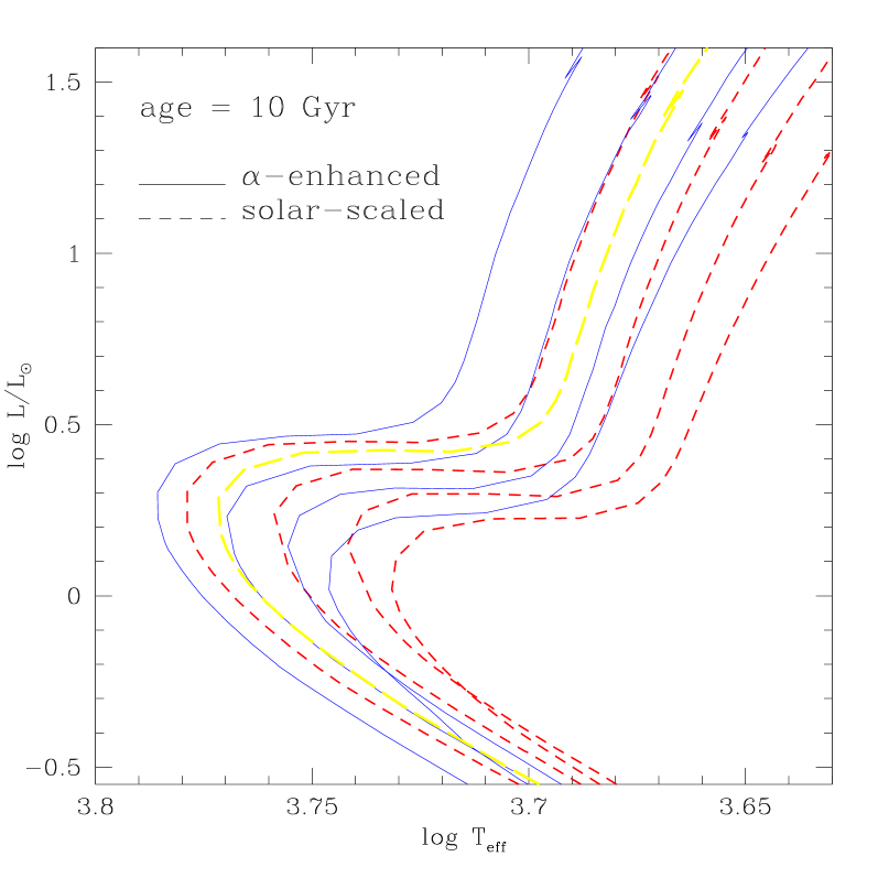
Figure 10: Comparison between $\alpha$-enhanced  (continuous lines) and solar-scaled (short-dashed lines) isochrones of 10 Gyr. In both cases, from left to right the metallicity values are $Z=0.008$, 0.019, 0.04, and 0.07. We also present a solar-scaled isochrone with $Z=0.011$ (long-dashed line), that has been obtained by interpolation among the solar-scaled tracks. This latter should be compared to the $\alpha$-enhanced  isochrone with $Z=0.019$ (see text).

Finally, one can ask whether an $\alpha$-enhanced isochrone may be approximated by a solar-scaled one with a slightly lower metallicity. In order to answer this question let us examine a set of 10 Gyr old isochrones. In Fig. 10 we plot all the isochrones with this age, and with metallicity going from $Z=0.008$ to $Z=0.07$ for both the $\alpha$-enhanced (continuous lines) and solar-scaled (short dashed lines) mixtures. One can see that both sets of isochrones have different shapes, the differences becoming larger at higher metallicities. More specifically, one can notice that the difference in effective temperatures at the turn-off point between an $\alpha$-enhanced isochrone and a solar-scaled one, $\Delta\mbox{$T\mbox{${}_{\rm eff}$}$}(\rm TO)$, increases with the metallicity, passing from $\Delta\mbox{$T\mbox{${}_{\rm eff}$}$}(\rm TO)=0.008$ to $0.015$ as $Z$ increases from 0.008 to 0.07. On the contrary, the temperature difference at the base of the RGB, $\Delta\mbox{$T\mbox{${}_{\rm eff}$}$}(\rm RGB)$, is almost constant and of about $\Delta\mbox{$T\mbox{${}_{\rm eff}$}$}(\rm RGB)\sim 0.019$.

For the same age we calculate, by interpolating among the grids of different metallicity, several solar-scaled isochrones with $Z$ spanning from $0.008$ to $0.019$, and selected among them the one best fitting the main sequence of the $Z=0.019$ $\alpha$-enhanced isochrone. This turns out to be the interpolated isochrone with $Z=0.011$, which is shown by the long-dashed line in Fig. 10. Clearly, this solar-scaled $Z=0.011$ isochrone does not reproduce well the RGB sequence of the $Z=0.019$ $\alpha$-enhanced one. More specifically, although $\Delta\mbox{$T\mbox{${}_{\rm eff}$}$}(\rm TO)$ is very small for this isochrone pair, $\Delta\mbox{$T\mbox{${}_{\rm eff}$}$}(\rm RGB)$ is not neglegible ($\Delta\mbox{$T\mbox{${}_{\rm eff}$}$}(\rm RGB)\sim 0.008$).

From this simple test we then conclude that for a fixed age and relatively high metallicities, an $\alpha$-enhanced isochrone cannot be reproduced by tuning the metallicity of a solar-scaled one.

The above temperature differences for RGB models (isochrones) bear very much on integrated spectral line indices of old metal-rich populations, which are commonly used to infer ages and metallicities of elliptical galaxies. This will be the subject of a forthcoming paper.

3.2 Theoretical Johnson and HST photometry

Theoretical luminosities and effective temperatures are translated to magnitudes and colours by means of extensive tabulations of bolometric corrections (BC) and colours obtained from properly convolving spectral energy distributions (SEDs) as a function of $T_{\rm eff}$, $\log g$ and [Fe/H]. The procedure is amply described in Bertelli et al. (1994), Bressan et al. (1994), and Tantalo et al. (1996) to whom the reader should refer for more details. Suffice it to recall here the following basic steps:

(i) The main body of the spectral library is from Kurucz (1992), however extended to the high and low temperature ranges. For stars with $\mbox{$T\mbox{${}_{\rm eff}$}$}>50,000$ K pure black-body spectra are assigned, whereas for stars with $\mbox{$T\mbox{${}_{\rm eff}$}$}<3500$ K the catalogue of stellar fluxes by Fluks et al. (1994) is adopted. This catalogue includes 97 observed spectra for all M-spectral subtypes in the wavelength range $3800\leq\mbox{\AA}\leq 9000$, and synthetic photospheric spectra in the range $9900\leq\mbox{\AA}\leq 12500$.

The scale of $T\mbox{${}_{\rm eff}$}$ in Fluks et al. (1994) is similar to that of Ridgway et al. (1980) for spectral types earlier than M4 but deviates from it for later spectral types. Since Ridgway’s et al. (1980) scale does not go beyond the spectral type M6, no comparison for more advanced spectral types is possible.

The problem is further complicated by possible effects of metallicity. The Ridgway scale of $T\mbox{${}_{\rm eff}$}$ is based on stars with solar metallicity ($Z\sim 0.02$) and empirical calibrations of the $T\mbox{${}_{\rm eff}$}$-scale for $Z\neq 0.02$ are not available.

To cope with this difficulty, we have introduced the metallicity-$T\mbox{${}_{\rm eff}$}$ relation of Bessell et al. (1989, 1991) using the ($V-K$) colour as a temperature indicator. An interpolation is made between the $T\mbox{${}_{\rm eff}$}$ of Bessell et al. (1989) and the ($V-K$) colours given by Fluks et al. (1994) for the spectral types from M0 to M10.

(ii) At a given metallicity [Fe/H], surface gravity $\log g$, and $T\mbox{${}_{\rm eff}$}$, BCs are determined by convolving the corresponding stellar SED with the response functions of the various pass-bands.

(iii) We recall that Kurucz does not provide atmospheric models for both solar-scaled and $\alpha$-enhanced mixtures. It is not therefore possible to estimate the impact (if any) of $\alpha$-enhanced atmospheres on the isochrone colours and magnitudes.

Johnson-Cousins photometry.

The response functions for the various pass-bands in which magnitudes and colours are generated are from the following sources: Buser & Kurucz (1978) for the $UBV$ pass-bands, Bessell (1990) for the $R$ and $I$ Cousins pass-bands, and finally Bessell & Brett (1988) for the $JHK$ pass-bands.

Re-normalization of the colours obtained by convolving the SEDs with pass-band, has been made by convolving the SED of Vega and imposing that the computed colours strictly match the observed ones (Kurucz 1992).

Finally, the zero point of the BCs is fixed by imposing that the BC for the Kurucz model of the Sun is $-0.08$.

HST-WFPC2 photometry.

The transformation to the WFPC2 photometric system (filters F170W, F218W, F255W, F300W, F336W, F439W, F450W, F555W, F606W, F702W, F814W, and F850LP) requires some additional explanations.

The main parameters defining this photometric system are given in Table 7. Columns (1) to (3) report the filter name, the mean wavelength $\bar{\lambda}$ and the r.m.s. band width (BW), respectively.

Table 7: Main characteristics of the WFPC2-HST photometric system and zero points.

Filter	$\bar{\lambda}$ (Å)	BW (Å)	$Z_{P}$	$m_{\rm ST}-m_{\rm VEGA}$	Note
(1)	(2)	(3)	(4)	(5)	(6)
F170W	1747	290	$-$20.6926	$-$0.4070	$-$
F218W	2189	171	$-$20.8737	$-$0.2263	$-$
F255W	2587	170	$-$21.0940	$-$0.0060	$-$
F300W	2942	325	$-$21.1336	+0.0336	Wide U
F336W	3341	204	$-$21.1876	+0.0876	U-John.
F439W	4300	202	$-$20.4325	$-$0.6675	B-John.
F450W	4519	404	$-$20.6339	$-$0.4661	Wide B
F555W	5397	522	$-$21.0798	$-$0.0202	V-John.
F606W	5934	637	$-$21.4250	+0.3250	Wide V
F702W	6862	587	$-$21.8594	+0.7594	Wide R
F814W	7924	647	$-$22.3309	+1.2309	I-John.
F850LP	9070	434	$-$22.7578	+1.6578	$-$

With the WFPC2 detector at least three kinds of magnitudes are commonly in use: $m_{\rm ST}$, $m_{\rm VEGA}$ and $m_{\rm AB}$ (see the Synphot User’s Guide by White et al. 1998, distributed by the STSDAS Group). In the following we limit ourselves to consider only the theoretical counterparts of $m_{\rm ST}$ and $m_{\rm VEGA}$.

For radiation with flat spectrum and specific flux $F_{P}$ (in ${\rm erg\,\,s^{-1}\,cm^{-2}\,\mbox{\AA}^{-1}}$) impinging on the telescope, the $m_{\rm ST}$ magnitude is defined by

$$m_{{\rm ST},P}=-21.1-2.5\log F_{P}$$ (1)

which means that $m_{{\rm ST},P}=0$ for $F_{P}=3.63\,10^{-9}$ $\rm erg\,\,s^{-1}\,cm^{-2}\,\mbox{\AA}^{-1}$.

Let us then define the pass-band $P(\lambda)$ as the product of the filter transmission by the response function of the telescope assembly and detector in use. In this case, $F_{P}$ is related to the counts rate $\dot{C}_{P}$ – i.e. the number of photons per second registered by the detector – through

$$F_{P}=\frac{hc}{A\int P(\lambda)\lambda\,\mbox{d}\lambda}\,\dot{C}_{P}$$ (2)

where $A$ is the effective collecting surface of the telescope, and $h$ and $c$ are the Planck constant and speed of light, respectively.

$\dot{C}_{P}$, the quantity actually measured at the telescope, can be easily converted to a specific flux by means of Eq. (2). Therefore, specific fluxes $F_{P}$ and $m_{{\rm ST},P}$ magnitudes can be defined for incoming spectra of any shape. In the case of a stellar source of radius $R$, located at a distance $d$, and emitting a specific flux $I_{\rm K}$, Eq. (1) can be replaced by

$$m_{{\rm ST},P}=-21.1-2.5\log\left[\frac{R^{2}}{d^{2}}\frac{\int P(\lambda)\,I_{\rm K}(\lambda)\,\lambda\,\mbox{d}\lambda}{\int P(\lambda)\,\lambda\,\mbox{d}\lambda}\right]$$ (3)

which defines the apparent $m_{{\rm ST},P}$ magnitude of a star.

In our case, we derive the absolute $M_{{\rm ST},P}$ magnitudes by simply locating our synthetic stars at a distance of $d=10$ pc in Eq. (3). The specific fluxes $I_{\rm K}(\lambda)$ are taken from the library of synthetic spectra in use as a function of $T_{\rm eff}$, surface gravity $g$, and chemical composition.

Similarly, we can define the $m_{{\rm VEGA},P}$ magnitudes

$$m_{{\rm VEGA},P}=Z_{P}-2.5\log\left[\frac{R^{2}}{d^{2}}\frac{\int P(\lambda)\,I_{\rm K}(\lambda)\,\lambda\,\mbox{d}\lambda}{\int P(\lambda)\,\lambda\,\mbox{d}\lambda}\right]$$ (4)

by imposing that the zero points $Z_{P}$ are such that the synthetic magnitudes of Vega match the ground-based $UBVRI$ Johnson apparent magnitudes for this star, for the filters which are closest in wavelength to each other (see column 6 in Table 7).

We adopt the values 0.02, 0.02, 0.03, 0.039, 0.035 mag for the apparent magnitudes of Vega in the $UBVRI$ Johnson system (see Holtzman et al. 1995). For the UV filters, Vega is assumed to have an apparent magnitude equal to zero.

We remind the reader that if we assume the apparent Vega magnitude to be equal to zero in all the pass-bands, we would obtain $Z_{P}=2.5\log F_{P,{\rm Vega}}$ and Eq. (4) would become

$$m_{{\rm VEGA},P}=-2.5\log\frac{F_{P}}{F_{P,{\rm Vega}}}$$ (5)

This latter is the definition of vegamag in the SYNPHOT package distributed with the STSDAS software. In this paper we do not make use of this calibration, but prefer to follow the slightly different one defined by Holtzman et al. (1995) and described above.

To get the final calibration, we insert in Eq. 4 the specific flux of Vega calculated by Castelli & Kurucz (1994) with atmosphere models, and converted it to an absolute flux on the Earth assuming for Vega the angular diameter of $3.24$ mas (Code et al. 1976). The absolute flux we have adopted differs (a few percent) from the one by Hayes (1985) used by Holtzman et al. (1995). Once more, the absolute magnitude $M_{{\rm VEGA},P}$ is obtained locating the synthetic star at a 10 pc distance. Column (4) of Table 7 lists the zero points we have obtained, whereas column (5) gives the difference $-21.1-Z_{P}$ between the zero point of the $m_{\rm ST}$ and $m_{\rm VEGA}$ magnitudes. The conversion from one magnitude scale to another is thus possible.

Finally, we calculate the bolometric corrections BC which allow one to convert theoretical bolometric magnitudes both to $M_{\rm ST}$ and $M_{\rm VEGA}$:

$${\rm BC}(P)^{M_{\rm ST}}_{T_{\rm eff},g} = M_{\rm bol}^{\odot}-2.5\log\left[\frac{4\pi(10{\rm pc})^{2}\sigma T_{\rm eff}^{4}}{L_{\odot}}\right]$$ (6)

$$+ 21.1+2.5\log\frac{\int P(\lambda)\,I_{\rm K}(\lambda)\,\lambda\,\mbox{d}\lambda}{\int P(\lambda)\,\lambda\,\mbox{d}\lambda}$$

$${\rm BC}(P)^{M_{\rm VEGA}}_{T_{\rm eff},g} = {\rm BC}(P)^{M_{\rm ST}}_{T_{\rm eff},g}-21.1-Z_{P}$$ (7)

where $\sigma$ is the Stefan-Boltzmann constant. For the solar luminosity and absolute bolometric magnitude we adopt $L_{\odot}=3.844\leavevmode\nobreak\ 10^{33}\leavevmode\nobreak\ \rm erg\leavevmode\nobreak\ s^{-1}$ (Bahcall et al. 1995) and $M_{\rm bol}^{\odot}=4.77$.

Owing to the presence of contaminants inside the WFPC2 (see Baggett & Gonzaga 1998 and Holtzman et al. 1995), $P(\lambda)$ changes slowly with time; in particular the UV throughput degrades, changing the photometric performances. To cope with this drawback, small corrections are usually added to the definition of the instrumental magnitudes in order to bring the magnitudes back to the optimal conditions (see Holtzman et al. 1995). Because of this, in the calculation of the bolometric corrections we do not use the present-day pass-bands $P(\lambda)$ provided by SYNPHOT but insert the pre-launch pass-bands, as in Holtzman et al. (1995).

3.3 Integrated magnitudes and mass-to-light ratios of single stellar populations

In this section we present the integrated magnitudes, colours and mass-to-light ratios for single stellar populations (SSP) of the same age and chemical compositions of the isochrones above, both in the Johnson-Cousins and WFPC2 photometric systems.

The integrated magnitudes and colours are computed assuming an initial mass function $\phi(M)$ and adopting the normalization

$$\int_{M_{\rm l}}^{M_{\rm u}}M\,\phi(M)\,\mbox{d}M=1\leavevmode\nobreak\ M_{\odot}$$ (8)

where $M_{\rm l}$ and $M_{\rm u}$ are the lower and upper limits of zero age main sequence stars. By doing so, the integrated magnitudes of these ideal SSPs can be easily scaled to produce integrated magnitudes for stellar populations of any arbitrary total initial mass $M_{\rm T,i}$, by simply adding the factor $-2.5\log M_{\rm T,i}$.

The theoretical mass-to-light ratios $M/L$ are calculated following the same procedure as in Alongi & Chiosi (1990) and Chandar et al. (1999).

The fate of a single star depends on its initial mass (binary stars are neglected here). In a brief and over-simplified picture of stellar evolution the following mass limits and groupings can be identified: (i) Stars more massive than $M_{\rm H}\simeq 0.7-0.8\leavevmode\nobreak\ M_{\odot}$ have a lifetime shorter than the current estimate of the Hubble age of the Universe, say $13-15$ Gyr. Stars lighter than this limit are not of interest here because once formed they live for ever. (ii) Stars more massive than $M_{\rm up}$ explode as supernovae leaving a neutron star remnant of $1.4\,M_{\odot}$. The possibility that massive stars ($M\geq 25\,M_{\odot}$) may end up as Black Holes is not considered here. (iii) Stars less massive than $M_{\rm W}$ and more massive than $M_{\rm H}$ terminate their evolution as White Dwarfs of suitable masses $M_{\rm WD}$ that depend on the initial mass and efficiency of mass loss during the RGB and AGB phases. With the current estimates of the mass loss efficiency $M_{\rm W}\simeq 5-6\,M_{\odot}$, i.e. $M_{\rm W}\simeq M_{\rm up}$. The possibility, however, exists that $M_{\rm W}<M_{\rm up}$. In such a case stars in the mass interval $M_{\rm W}$ to $M_{\rm up}$ reach the C-ignition stage and deflagrate as supernovae leaving no remnant. For the purposes of the present study, this latter case is neglected and $M_{\rm W}=M_{\rm up}$ is always assumed. Finally, let $M_{\rm a}$ be the initial mass of the most massive star still alive in a SSP of a certain age. It is worth recalling that all the above mass limits depend on the initial chemical composition and that this dependence can be properly taken into account.

Therefore, at any given age $t$ the total mass $M_{\rm T}$ of a SSP is made of two contributions:

$$M_{\rm T}(t)=\int_{M_{\rm l}}^{M_{\rm a}}M\,\phi(M)\,\mbox{d}M+\int_{M_{\rm a}}^{M_{\rm u}}M_{\rm r}\,\phi(M)\,\mbox{d}M$$ (9)

where the first right-hand side term is the total mass of the stars still alive at the age $t$ (i.e. burning a nuclear fuel) and the second one is the total mass in stellar remnants, i.e. white dwarfs or neutron stars depending on the initial mass of the progenitor (i.e. $M_{\rm r}(M)=M_{\rm WD}(M)$ for $M\leq M_{\rm up}$, and $M_{\rm r}(M)=1.4\leavevmode\nobreak\ M_{\odot}$ for $M>M_{\rm up}$). We adopt an upper mass limit $M_{\rm u}=120\leavevmode\nobreak\ M_{\odot}$. The choice for the lower mass limit, $M_{\rm l}$, is explained below. It is worth recalling here that, due to eq. 8, $M_{\rm T}(t)$ is the current mass of an ideal SSP with initial mass equal to $1\leavevmode\nobreak\ M_{\odot}$. $M_{\rm T}(t)$ decreases as a function of time from its initial value, due to the mass lost by both stellar winds (for all masses) and supernova explosions (from massive stars).

Finally, the total luminosity $L_{j}$ of the SSP in any pass-band $j$ is obtained by integrating, along the isochrone, the luminosity of individual stars whose number is given by the IMF

$$L_{j}=\int_{M_{\rm l}}^{M_{\rm a}}L_{j}(M)\,\phi(M)\,\mbox{d}M\leavevmode\nobreak\ .$$ (10)

To proceed further, one has to specify the initial mass function and $M_{\rm l}$. Here, we adopt the Salpeter (1955) law with slope $x=1.35$ over the whole mass range $M_{\rm l}$ to $M_{\rm u}$. Concerning $M_{\rm l}$, the choice $M_{\rm l}=0.068\leavevmode\nobreak\ M_{\odot}$ is made by imposing that the observational value $M/L_{V}=0.19\pm 0.04$ of the LMC cluster NGC 1866 is matched (see Girardi & Bica 1993). The age and metallicity of NGC 1866 are $10^{8}$ years and $Z=0.008$, respectively, whereas its $M/L_{V}$ is close to the mean value of 0.20 for LMC clusters of the same age (see Battinelli & Capuzzo-Dolcetta 1989, and references therein).

4 Concluding remarks

We have computed extended sets of $\alpha$-enhanced evolutionary tracks and isochrones at relatively high metallicities. A major improvement, with respect to previous calculations of $\alpha$-enhanced tracks, is that we made use of self-consistent opacities, i.e. computed with the same $\alpha$-enhanced chemical compositions over the complete range of temperatures. The main result is that in general all evolutionary phases (isochrones) have higher effective temperature with respect to solar-scaled models (isochrones) of same metal content $Z$. The temperature shift is caused by the lower opacities of the $\alpha$-enhanced mixtures. Moreover, we find that at relatively high metallicities and old ages, an $\alpha$-enhanced isochrone cannot be mimicked by simply using a solar-scaled isochrone of lower metallicity.

Obvious limitation of the present results is that they refer to a particular choice for the $\alpha$-enhanced chemical compositions derived from observations of a particular sample of metal-poor field stars. Future observational data may suggest a different partition of metals in $\alpha$-enhanced stars, and hence different results for the stellar models and corresponding isochrones.

Testing a large number of possible combinations of $\alpha$-enhanced ratios, though feasible, would not be of practical use owing to the present uncertainty on the abundance ratios. Therefore, the results of this study ought to be taken as indicative of the potential effect of $\alpha$-enhanced element ratios.

Moreover, it is likely that variations of single $\alpha$-elements are less important than the whole problem of including or not the enhancement of $\alpha$-elements in the initial chemical composition. Finally, it is still not clear whether differences in enhancements are significant compared to the errors in the determinations.

Retrieval of the data sets.

Complete tabulations of the relevant data for all evolutionary sequences, isochrones, integrated magnitudes and colours and mass-to-light rations together with useful summary tables can be obtained either upon request to the authors or downloaded from the address http://pleiadi.pd.astro.it.

The layout of the tables of stellar models and isochrones is the same as in Girardi et al. (2000) as far as the Johnson-Cousins photometric system is concerned. For the WFPC2 system the layout is similar, with table headers allowing to easily identify the pass-band.

Acknowledgments. We like to thank A. Bressan for many suggestions and useful conversations, H. Schlattl for his help with the opacity interpolation code, H. Aussel and M. Zoccali for their useful clarifications about the HST/WFPC2 photometric system, J. Holtzman for providing us with the pre-launch WFPC2 pass-bands, and the anonymous referee for useful suggestions. L.G. acknowledges support from the Alexander von Humboldt-Stiftung during his stay at MPA. B.S. thanks MPA for the warm hospitality and support. This study has been funded by the Italian Ministry of University, Scientific Research and Technology (MURST) under contract “Formation and Evolution of Galaxies” n. 9802192401.

References

Alexander D.R., Ferguson J.W., 1994, ApJ 437, 879

Alongi M., Chiosi C., 1990, in Astrophysical Ages and Dating Methods, ed. E. Vangioni-Flam et al. (Gif-sur-Yvette: Editions Frontières), 207

Alongi M., Bertelli G., Bressan A., Chiosi C., 1991, A&A 244, 95

Anders E., Grevesse N., 1989, Geochim. Cosmochim. Acta, 53,197

Baggett S., Gonzaga S., 1998, ISR WFPC2 98-03

Bahcall J.N., Pinsonneault M.H., Wasserburg G.J., 1995, Rev. Mod. Phys. 67, n.4, 781

Battinelli P., Capuzzo-Dolcetta R., 1989, ApJ 347, 794

Bertelli G., Bressan A., Chiosi C., Fagotto F., Nasi E., 1994, A&AS 106, 275

Bessell M.S., 1990, PASP 102, 1181

Bessell M.S., Brett J.M., 1988, PASP 100, 1134

Bessell M.S., Brett M.J., Wood P.R., Scholz M., 1989, A&AS 77, 1

Bessell M.S., Brett M.J., Wood P.R., Scholz M., 1991, A&AS 87, 621

Böhm-Vitense E., 1958, Z. Astroph. 46, 108

Bressan A., Bertelli G., Chiosi C., 1981, A&A 102, 25

Bressan A., Fagotto F., Bertelli G., Chiosi C., 1993, A&AS 100, 647

Bressan A., Chiosi C., Fagotto F., 1994, ApJS 94, 63

Buser R., Kurucz R.L. 1978, A&A 70, 555

Carney B.W., 1996, PASP, 108, 900

Catelan M., De Freitas Pacheco J.A., Horvath J.E., 1996, ApJ, 461, 231

Cassisi S., Castellani V., Degl’ Innocenti S., Weiss A., 1998, A&AS 129, 267

Castelli F., Kurucz R.L., 1994, A&A 281, 817

Castellani V., Degl’Innocenti S., Girardi L., et al., 2000, A&A 354, 150

Caughlan G.R., Fowler W.A., 1988, Atomic Data Nucl. Data Tables 40, 283

Chandar R., Bianchi L., Ford H.C., Salasnich B., 1999, PASP 111, 794

Chiosi C., Vallenari A., Bressan A., 1997, A&AS 121, 301

Code A.D., Bless R.C., Davis J., Brown R.H., 1976, ApJ, 203, 417

Fagotto F., Bressan A., Bertelli G.P., Chiosi C., 1994, A&AS 105, 29

Fluks M.A, Plez B., The P.S., et al., 1994, A&AS 105, 311

Girardi L., 1999, MNRAS 308, 818

Girardi L., Bica E., 1993, A&A 274, 279

Girardi L., Bertelli G., 1998, MNRAS 300, 533

Girardi L., Bressan A., Bertelli G., Chiosi C., 2000, A&AS 141, 371

Grevesse N., Noels A., 1993, Phys. Scr. T, 47, 133

Haft M., Raffelt G., Weiss A., 1994, ApJ 425, 222

Hayes D.S., 1985, Calibration of fundamental stellar quantities, IAU Symposium 111, ed. D.S. Hayes, L.E. Pasinetti and A.G.D. Philip (Dordrecht, Reidel), p. 225

Holtzman J.A., Burrows C.J., Casertano S., et al., 1995, PASP, 107, 1065

Hubbard W.B., Lampe M., 1969, ApJS 18, 297

Iglesias C. A., Rogers F. J., 1993, ApJ 412, 752

Iglesias C. A., Rogers F. J., 1996, ApJ 464, 943

Itoh N., Mitake S., Iyetomi H., Ichimaru S., 1983, ApJ 273, 774

King J., 1994, PASP, 106,423

Kurucz R.L., 1992, in IAU Symp. 149: The Stellar Populations of Galaxies, eds. B. Barbuy, A. Renzini, Dordrecht, Kluwer, p. 225

Landré V., Prantzos N., Aguer P., et al., 1990, A&A 240, 85

Matteucci F., Brocato E., 1990, ApJ 365, 539

Matteucci F., Romano D., Molaro P., 1999, A&A 341, 458

McWilliam A., Rich R.M., 1994, ApJS, 91,749

Mihalas D., Hummer D.G., Mihalas B.W., Däppen W., 1990, ApJ 350, 300

Munakata H., Kohyama Y., Itoh N., 1985, ApJ 296, 197

Rich R.M., McWilliam A., 2000, in Discoveries and Research Prospects from 8–10-Meter-Class Telescopes, Proc. of the SPIE vol. 4005, ed. J. Bergeron, in press (astro-ph/0005113)

Ridgway S.T., Joyce R.R., White N.M., Wing R.F., 1980, ApJ 235, 126

Rogers F.J., Iglesias C.A., 1992, ApJS 79, 507

Rogers F.J., Iglesias C.A., 1995, in ASP Conf. Proc. 78, Astrophysical Applications of Powerful New Databases, ed. S.J. Adelman, W.L. Wiesse (San Francisco:ASP), 31

Ryan S.G., Norris J.E., Bessel M.S., 1991, AJ 102, 303

Salaris M., Weiss A., 1998, A&A 335, 943

Salaris M., Chieffi A., Straniero O., 1993, ApJ 414, 580

Salaris M., Degl’Innocenti S., Weiss A., 1997, ApJ 479, 665

Salpeter E.E, 1955, ApJ 121, 161

Schlattl H., Weiss A., 1998, in ”Proc. Neutrino Astrophysics” , Ringberg Castle, Tegernsee, Germany, 20-24 Oct 1997, ed. M. Altmann, W. Hillebrandt, H.-T.Janka and G.Raffelt (SFB Astroteilchenphysik, Technical University Munich)

Späth H., 1973, in ”Spline-Algorithmen zur Konstruktion glatter Kurven und Flächen”, München: Oldenbourg.

Tantalo R., Chiosi C., Bressan A., Fagotto F., 1996, A&A 311, 361

VandenBerg D.A., Swenson F.J., Rogers F.J., Iglesias C.A., Alexander D.R., 2000, ApJ 532, 430

Weiss A., Keady J.J., Magee N.H. Jr., 1990, Atomic Data and Nuclear Data Tables 45, 209

Weiss A., Peletier R.F., Matteucci F., 1995, A&AS 296, 73

White R., Greenfield P., Kinney E. et al., 1998, ed. by Association of Universities for Research in Astronomy, Inc.

Worthey G., Faber S.M., Jesús González J., 1992, ApJ 398, 69