Optimizing the angular resolution of the HEGRA telescope system to study the emission region of VHE gamma rays in the Crab Nebula

Abstract

The HEGRA system of imaging atmospheric Cherenkov telescopes provides for specially selected classes of events an angular resolution of better than 3’. By comparing the measured angular distribution of TeV gamma rays from the Crab Nebula with the distribution expected on the basis of Monte Carlo simulations, and with measurements of gamma rays from the point source Mrk 501, we conclude that the rms size of the VHE gamma-ray emission region in the Crab Nebula is less than 1.5’.

1 Introduction

Stereoscopic systems of imaging atmospheric Cherenkov telescopes (IACTs) such as the HEGRA IACT system (Daum et al. hegra_perf (1997)) allow to reconstruct the directions and energies of TeV gamma-rays with high precision. The analysis techniques, the control of systematics, and the understanding of the angular resolution function of the instrument (Pühlhofer et al. hegra_pointing (1997), Aharonian et al. 1999b , Hofmann et al. hegra_reco (1999)) has progressed to a level that one can start to study the characteristics of extended sources on a scale of a few arcminutes. These scales start to become interesting in disentangling the emission mechanisms for Galactic TeV gamma-ray sources such as the Crab Nebula or the pulsar PSR B1706-44. In this paper, we present, as a case study, an investigation of the size of the emission region of the Crab Nebula at TeV energies.

The Crab Nebula is one of the best-studied objects in the sky, in all wavelength regimes. It has been established as a TeV gamma-ray source by the Whipple group, using the imaging atmospheric Cherenkov technique (Weekes et al. weekes (1989), Vacanti et al. vacanti (1991)), and has been studied with many other Cherenkov telescopes. The precise spectral shape of gamma-ray emission from the Crab Nebula has been the subject of a number of recent publications (Hillas et al. whipple_c (1998), Tanimori et al. cangaroo (1998), Konopelko 1999a ). The spectrum is consistent with a power-law extending from a few 100 GeV out to energies of 50 TeV and beyond. Contrary to observations in the X-ray and GeV gamma-ray regimes, the TeV gamma-ray emission does not show a pulsed component attributable to a direct contribution from the Crab Pulsar; pulsed emission is below 3% of the DC flux (Aharonian et al. 1999c , Burdett et al. whipple_pulsar (1999)). The commonly accepted model for VHE gamma-ray production in the Crab Nebula assumes electron acceleration in the termination shock of the pulsar wind at a distance of about 0.1 pc (0.2’) from the pulsar (see, e.g., Kennel & Coroniti (coroniti_crab (1984)), De Jager & Harding (harding_crab (1992)), Atoyan & Aharonian (aharonian_crab (1996)), Aharonian & Atoyan (review (1998))). The electrons diffuse out into the Nebula and produce a characteristic two-component electromagnetic spectrum: synchrotron emission dominates at most energies up to about 0.1 GeV, whereas the inverse Compton process generates higher-energy gamma-rays with energies from the GeV range up to 100 TeV and beyond. From the relative strength of the two components, values for the average magnetic field of 15 - 30 nT have been derived (Hillas et al. whipple_c (1998), De Jager & Harding harding_crab (1992), Atoyan & Aharonian aharonian_crab (1996)).

The Crab Nebula represents an extended source of electromagnetic radiation. Since the electrons loose energy as they expand out into the Nebula, primarily due to synchrotron losses, the effective source size is predicted to shrink with increasing energy of the radiation, with radio emission extending up to and beyond the filaments visible in the optical, whereas hard X-rays and multi-TeV gamma-rays should be produced primarily in the direct vicinity of the shock (see, e.g., Kennel & Coroniti (coroniti_crab (1984)), De Jager & Harding (harding_crab (1992)), Atoyan & Aharonian (aharonian_crab (1996)), Amato et al. (amato (1999))). At TeV energies, a second production mechanism for gamma-rays could be the hadronic production by protons accelerated in the shock (Atoyan & Aharonian aharonian_crab (1996)) or resulting from decays of secondary neutrons produced in the pulsar magnetosphere (Bednarek & Protheroe bednarek (1997)); gamma rays are produced in interactions with the surrounding material, e.g. in the filaments (Atoyan & Aharonian aharonian_crab (1996)). This contribution might be enhanced due to a trapping of protons in local magnetic fields associated with the filaments, increasing the interaction probability. Given that the size of the Crab Nebula – with its about 4’ by 3’ extension in the optical – is comparable to the angular resolution achieved for TeV gamma rays by the HEGRA system of imaging atmospheric Cherenkov telescopes (IACTs), a study of the size of the TeV emission region of the Crab Nebula is now possible with meaningful sensitivity. This paper reports such an analysis, based on data collected over the last years with the HEGRA IACT system.

For comparison and later reference, we will briefly summarize the existing information on the size of the Crab Nebula, as a function of the energy of the radiation. An obvious problem in such a compilation is that there is no unique definition of ‘size’. For comparison with the TeV results given later, the most relevant quantity is an rms size, gained by approximating the intensity distribution by a two-dimensional Gaussian, or by directly calculating the rms width by projecting or slicing the intensity distribution along an axis, and averaging over directions. Rms width values based on 5 GHz radio data (Wilson wilson (1972)), optical data from Woltjer (woltjer (1957)) as displayed in Wilson (wilson (1972)), and 0.1 - 4.5 keV X-ray data (Harnden & Seward harnden (1984)) are compiled in Hillas et al. (whipple_c (1998)). Additional rms values were obtained for the 327 MHz radio data of Bietenholz et al. (bietenholz (1997)), and for the 22 - 64 keV X-ray data of Makishima et al. (makishima (1981)). These data are shown in Fig. 1 as full circles.

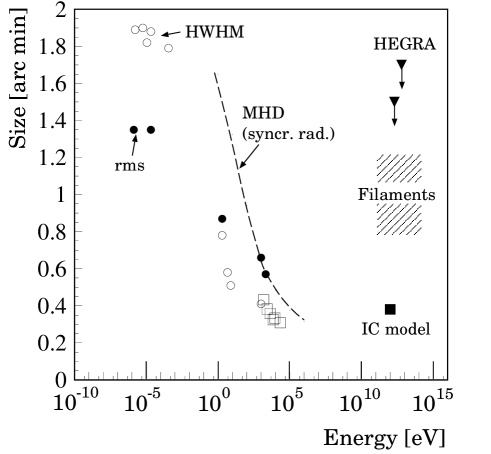
Figure 1: Angular size of the Crab nebula at different frequencies. Full circles: rms size, averaged over directions. Open circles: half width at half maximum (HWHM, defined as FWHM/2), averaged over the long and short axis. Open squares: HWHM along the $300^{\circ}$ direction. See text for references. The dashed line indicates the frequency dependence of the size of the (synchrotron-radiation) emission region as given by Kennel & Coroniti (coroniti_crab (1984)), and the full square shows the rms size predicted for inverse-Compton gamma-rays at TeV energy (Atoyan & Aharonian aharonian_crab (1996)). The dashed region indicates the rms size range of the filaments, the likely scale for hadronic production mechanisms. The triangles show the upper limits on the rms source size at TeV energies derived in this work.

The bulk of the size values quoted in the literature refer to a different measure, the full width at half maximum (FWHM), which unfortunately in case of a structured intensity distribution depends also on the resolution of the instrument. In some cases, data are only available along a specific direction, and do not allow to average over the long and short axis of the Nebula. In particular in earlier X-ray data, the contributions of the pulsar and of the surrounding nebula are not separated. Fig. 1 includes (as open circles) FWHM size data, averaged over the long and short axis, at radio wavelengths (Wilson wilson (1972)) and in the optical, NUV, FUV, and X-ray, as given in Hennessy et al. (hennessy (1992)). Also shown are X-ray data compiled in Ku et al. (ku (1976)), which refer to the width along the $300^{\circ}$ direction (open squares). A clear trend for decreasing source size with increasing energy is evident, considering either the rms size values, the averaged FWHM size values, and the fixed-direction X-ray widths. Included as dashed line is the frequency dependence of the synchrotron emission region as sketched in Kennel & Coroniti (coroniti_crab (1984)). The size of the emission region for inverse-Compton TeV gamma rays can be predicted using the average magnetic field to relate synchrotron photon energies to electron energies and to inverse-Compton gamma rays; from such arguments, one concludes that the size for TeV gamma-rays should correspond to the X-ray size. The rms size predicted for the TeV gamma-ray emission region by the detailed calculations of Atoyan & Aharonian (aharonian_crab (1996)) is included in Fig. 1. Basically, inverse-Compton TeV gamma-rays should emerge from the toroidal X-ray emission region clearly visible in the ROSAT data (Hester et al. hester (1995)) and in the recent Chandra image (Weisskopf et al., 2000), as already speculated earlier by Aschenbach & Brinkmann (aschenbach (1975)). The projected semi-major and semi-minor axes of the emission torus are 38” and 18”, respectively. Due to the nonuniform strength of X-ray emission along the torus, the resulting emission profile is roughly elliptical, and its center is shifted N relative to the pulsar location by about 0.3’. Hadronic production mechanisms are expected to generate larger source sizes, of the scale of the size of the nebula (shaded region in Fig. 1).

2 Observations of the Crab Nebula with the HEGRA CT system

The HEGRA system of imaging atmospheric Cherenkov telescopes is located on the Canary Island of La Palma, on the site of the Observatorio del Roque de los Muchachos. The telecope system consists of five telescopes, with a mirror area of 8.5 m² and a focal length of 5 m. A sixth prototype telescope is operated in stand-alone mode and is not used for the analysis presented here. The system telescopes are arranged at the corners and in the center of a square of about 100 m side length. The alt-azimuth mounted telescopes are equipped with cameras consisting of 271 photomultipliers (PMTs). Each PMT views an area of the sky of $0.25^{\circ}$ diameter; the field of view of each camera is about $4.3^{\circ}$. Cherenkov images of air showers are recorded whenever two telescopes trigger simultaneously; the trigger condition requires that two neighboring PMTs exhibit signals equivalent to 8 or more photoelectrons. Typical trigger rates are around 15 Hz, for an energy threshold of 500 GeV for vertical gamma rays. Details about the HEGRA IACTs and their performance can be found in Daum et al. (hegra_perf (1997)), Aharonian et al. (1999b ), Hermann (hegra_camera (1995)), Bulian et al. (hegra_trigger (1998)).

The Crab Nebula was observed in each season since the HEGRA IACT system commenced operation in late 1996, initially with three telescopes, later with four and since late 1998 with the complete set of five telescopes. For this analysis, only data taken in the years 1997 and 1998 were used, acquired with at least four telescopes under good weather conditions; in order to be able to compare with earlier Mrk 501 data taken with four telescopes, data from the fifth telescope was not used in the most recent five-telescope data sets. The quality-selected data set amounts to an integral observation time of about 155 h, and includes about 6.3 million events. For the final analysis, only data taken at zenith angles of less than $30^{\circ}$ were included, with about 3.5 million events remaining.

The Crab Nebula was observed in the so-called wobble mode, with the source offset by $0.5^{\circ}$ in declination relative to the telescope axes. The sign of the offset alternated every 20 min. A region offset by the same amount, but in the opposite direction, is used for background estimates, avoiding the need for special off-source observations. Since the stereoscopic reconstruction of air showers provides an angular resolution of typically 6’, signal and background regions are well separated.

The techniques for data analysis are similar to those documented, e.g., in Aharonian et al. (1999b ,1999d ). Direction and impact point of an air shower are reconstructed from the stereoscopic views of the shower. Based on the measured impact point and the known (Aharonian et al. 1999a ) distribution of Cherenkov light as a function of the distance to the shower axis, an energy estimate is derived, with a typical resolution of 20%. Gamma-ray candidates are selected on the basis of image shapes. Given the core distance and the intensity (the Hillas size parameter (Hillas hillas_param (1985))), the expected width of a gamma ray image is determined. The measured width values are normalized to this value, and averaged over telescopes. A cut on the resulting mean scaled width $<$ 1.2 retains most gamma-rays, but rejects the bulk of the cosmic-ray showers.

In detail, the reconstruction of shower geometry differs somewhat from the techniques used so far. Whereas the normal reconstruction procedure combines images from all telescopes regardless of their quality, the new procedure assigns – on the basis of the Monte Carlo simulations of Konopelko et al. (1999b ) – errors to the relevant image parameters (the location of the image centroid and the orientation of the image axis). These errors depend on the intensity and the shape of the images and are propagated through the geometrical reconstruction, resulting in error estimates (or, to be precise, a covariance matrix) for the shower parameters. Details of the algorithm are given in Hofmann et al. (hegra_reco (1999)). Depending on the characteristics of an event, an angular resolution between 2’ and more then 10’ is predicted, with average value slightly below 6’ . The ability to select subsets of events with better-than-average resolution will be used extensively in the analysis of the size of the VHE emission region in the Crab Nebula.

3 The limit on the size of the emission region

Even if the size at radio wavelengths – about 1.3’ rms – is used as a most extreme possibility for the size at TeV energies, the source size $\sigma_{s}$ is still smaller than the angular resolution $\sigma_{o}$ for the best subsets - about 2’ to 3’. Therefore, one cannot expect to generate a detailed map of the source. Instead, an extended emission region of (rms) size $\sigma_{s}$ would primarily show up as a slight broadening of the angular distribution of gamma-rays, beyond the value determined by the experimental resolution:

$$\sigma=\sqrt{\sigma_{o}^{2}+\sigma_{s}^{2}}$$ (1)

or, for $\sigma_{s}$ small compared to $\sigma_{o}$,

$${\Delta\sigma\over\sigma_{o}}={\sigma-\sigma_{o}\over\sigma_{o}}\approx{\sigma_{s}^{2}\over 2\sigma_{o}^{2}}$$ (2)

For an intrinsic resolution of 3’ (in a projection) and a 1.5’ rms source size, one would find a 3.4’ wide angular distribution; for the 6’ resolution, the resulting width is 6.2’. In order to positively detect a finite source size, or to derive stringent upper limits, one has (a) to measure the width of the angular distribution of gamma-rays with sufficient statistical precision, and (b) to quantitatively understand the response function of the instrument at the same level, and to control systematic effects which influence the resolution.

For a given number $n$ of events from the source, and ignoring for the moment the effect of background under the signal, the statistical error on the width of the (projected) angular distribution is $\Delta\sigma/\sigma=1/(2n^{1/2})$. In case the angular distribution is consistent with a point source, Eqn. 2 then implies a (1 standard deviation) upper limit $\sigma_{s}<\sigma_{o}n^{-1/4}$. Therefore, one will want to minimize $\sigma_{o}$ by selecting a subset of events with particularly well-determined directions, even at the expense of event statistics. More critical are, in general, systematic errors. Pointing imperfections, changes in mirror alignment, etc. can cause differences in the angular resolution between data sets taken at different times, under different conditions, and between the data and the simulation. If, e.g., the intrinsic resolution of the instrument is known and reproducible to 10%, the minimum source size which can be reliably detected is $0.46\sigma_{o}$, according to Eqs. 1 or 2. Once more, a selection towards small $\sigma_{o}$ is preferred. Among gamma-ray events, we find that about 1% of the events have a predicted resolution below 1.8’ ($0.03^{\circ}$), 6% below 2.4’ ($0.04^{\circ}$), 15% below 3’ ($0.05^{\circ}$), and 60% below 6’ ($0.1^{\circ}$), respectively. In particular the samples with resolutions better than 2.4’ or 3’ combine good angular resolution with acceptable statistics. The cuts on angular resolution have the additional benefit on enhancing the gamma-ray sample relative to the cosmic-ray background; cosmic-ray showers generate more diffuse images and have a worse angular resolution. Fig. 2 shows the angular distribution of events retained after a cut at 3’ resolution in both projections, applying only very loose additional cuts on event shapes (a cut on the mean scaled width at 1.2, which retains over 80% of the gamma-ray events). The selection also biases the sample towards higher energies, since high-energy events produce more intense images, with smaller errors on the image parameters. In the overall data sample, the median energy of reconstructed events is 0.9 TeV; after a cut on the resolution at 3’, this value rises to 2.0 TeV.

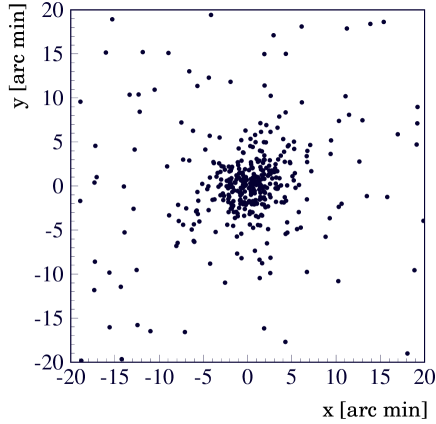
Figure 2: Angular distribution of reconstructed showers in a local coordinate system centered on the Crab pulsar. Events were selected on the basis of the predicted angular error ($<$ 3’ in both directions) and on the basis of image shapes (mean scaled width $<1.2$).

While the evaluation of statistical errors is straight forward, the control of systematic errors is more difficult. The pointing of the telescopes is referenced to and corrected offline on the basis of star images (Pühlhofer et al. hegra_pointing (1997)), and the achievable pointing precision has been investigated in considerable detail. We are confident to achieve a pointing deviation of less than $\pm 0.5^{\prime}$ in each coordinate. Indeed, when the Crab data set was subdivided into seasonal subsets, the reconstructed source position was in all cases consistent with the nominal source location – the position of the Crab pulsar.

Table 1: Width of the angular distribution of events relative to the source, comparing the Mrk 501 and Crab data sets with Monte Carlo simulations using the measured gamma-ray energy spectrum as an input. Data sets are selected according to the estimate of the angular resolution, as provided by the shower reconstruction algorithm. The quoted width values are derived using a Gaussian fit to the projected angular distribution. For the last two rows of the table, only the central part of the distribution is fit; there are significant non-Gaussian tails (both in the Monte Carlo and in the data).

Selection on	Mrk 501 MC	Mrk 501 data	Crab MC	Crab data
angular resolution [arc min]	[arc min]	[arc min]	[arc min]	[arc min]
$\leq$ 2.4	$2.43\pm 0.05$	$2.46\pm 0.06$	$2.41\pm 0.05$	$2.41\pm 0.14$
$\leq$ 3	$2.81\pm 0.04$	$2.83\pm 0.05$	$2.81\pm 0.04$	$2.70\pm 0.10$
$\leq$ 6	$3.58\pm 0.03$	$3.63\pm 0.04$	$3.64\pm 0.04$	$3.70\pm 0.09$
all events	$4.23\pm 0.04$	$4.26\pm 0.04$	$4.30\pm 0.04$	$4.37\pm 0.10$

To evaluate the level at which the angular resolution is understood, we use the sample of gamma-rays from the AGN Mrk 501 as a reference set (see Aharonian et al. (1999b , 1999d ) for details on this data set), assuming that Mrk 501 represents a point source. Table 1, columns 2,3 compare the measured angular distribution for different subsets of events with the Monte-Carlo predictions. ‘Angular resolution’ again refers to the Gaussian width of the projected angular distribution of events. Excellent agreement between data and Monte-Carlo is seen for all data sets. We note that the resolution estimates given by the reconstruction algorithm are low by 10% to 15%, for the samples selected for good resolution. The $\leq$ 2.4’ sample, e.g., should show a 2.2’ resolution, compared to the measured value of 2.46’. Given the relatively crude parametrization of image parameter errors used in the reconstruction (Hofmann et al., hegra_reco (1999)), a deviation at this level is not unexpected, and in any case the effect is fully reproduced by the simulations.

After these preliminaries, we can now address the Crab data set. Fig. 3(a) shows the background-subtracted angular distribution of reconstructed showers relative to the source direction, projected onto the axes of a local coordinate system, after a cut on the estimated error of less than 3’. Superimposed is the corresponding distribution of Monte-Carlo events, generated with the measured Crab spectrum. Fig. 3(b) shows the corresponding comparison with gamma-rays from Mrk 501. In particular after the selection on good angular resolution, the two event samples are very similar in their characteristics (mean predicted resolution, mean number of telescopes contributing to the reconstruction, etc.) and can be compared directly, despite the differences in the energy spectrum of the two sources. Table 1, cols. 4,5 list the widths of the distributions for the Crab gamma-rays, and the corresponding simulations. In general, we find, within the statistical errors, good agreement between the Crab and Mrk 501 data sets, and between Crab data and Monte-Carlo.

Another option to allow a direct comparison of the Mrk 501 and Crab data sets is not to look at the angular deviations $(x,y)$ between a gamma-ray and the source, but rather to normalize these quantities with the angular resolutions $\sigma_{o,x},\sigma_{o,y}$ predicted event-by-event by the reconstruction algorithm. Ideally, one expects to see a Gaussian distribution of unit width, independently of the energy spectrum, the number of telescopes active for a given data set, etc. The observed distributions are indeed Gaussian; as mentioned above, their widths differ by up to 10% to 15% from unity, depending on the selection of events. Most importantly, however, these width values are consistent between all four sets of events (Mrk 501 MC, Mrk 501 data, Crab MC, Crab data), within errors of 1.5% or less for the large-statistics sets where all events are included. This agreement demonstrates that there are no uncontrolled systematic effects between the two experimental data sets, or between the experimental data and the simulations.

Figure 3: (a) Full points: background-subtracted angular distribution of gamma-rays, projected onto the axes $(x,y)$ of a local coordinate system centered on the Crab pulsar. Events are selected to provide an angular resolution of better than 3’. Superimposed, as open points, the corresponding distribution of Monte-Carlo events, normalized to the same area. (b) Comparison of the angular distributions of gamma rays from the Crab Nebula (full points) and from Mrk 501 (open points).

Since the width of the angular distribution of gamma-rays from the Crab Nebula is consistent with the expected width, and with the width observed for Mrk 501, we can only give an upper limit on the source size. Taking into account the statistical errors on the Crab sample and on the reference samples, we find – following Caso et al. (pdg (1998)) – 99% confidence level upper limits of 1.0’ for the sample with a cut at 3’ resolution, and 1.3’ for the $\leq$ 2.4’ sample. To be conservative, and since it was always planned to use the $\leq$ 2.4’ sample as a safest compromise between statistical and systematic uncertainties, we adopt the 1.3’ limit. Adding in additional systematic uncertainties due to pointing precision, we quote a final limit of 1.5’ for the rms source size at a median energy of 2 TeV.

A possible contribution of gamma-rays from hadronic processes is generally expected to be most relevant at higher energies, in the 10 TeV to 100 TeV range. Therefore, the source size was also studied for an event sample with reconstructed energies above 5 TeV; data are consistent with a point source and the corresponding limit on the rms source size is 1.7’. Limited statistics prevent studies at even higher energies.

The elliptical shape of the X-ray emission region suggests to perform the same analysis in a rotated coordinate system, with its axes aligned along the major and minor axes of the X-ray profile. Results obtained for the width in the major and minor direction do not show any significant difference. Given the fact that the limits are large compared to the (rms-)size of the X-ray emission region, this observation is not surprising. The TeV source is reconstructed 0.2’ from the location of the pulsar, and is consistent both with the location of the pulsar, and with the center of gravity of the X-ray emission region, within the systematic errors in the telescope pointing (less than $\pm 0.5^{\prime}$ in each coordinate). While the statistical error alone is small enough to resolve a shift of 0.3’ as observed in the X-ray image, current systematic errors prevent such a measurement at TeV energies.

The limits obtained in this work are included in Fig. 1.

We note in passing that also the widths of the distributions obtained for the AGN Mrk 501 are consistent with MC expectations, indicating the absence of a halo on the arcminute scale. Potential halo types for AGNs include wide pair halos (Aharonian, Coppi & Völk 1994) or narrow halos caused by intergalactic magnetic fields (Plaga 1995). For a relatively near source such as Mrk 501, a pair halo would be much wider than the field of view of the camera and could not be detected as an increased apparent source size; the other type of halo speculated in (Plaga 1995) would be well below our resolution. We do not see any time-dependence of the source size, or any correlation with the TeV gamma-ray flux. Details will be given elsewhere.

4 Concluding remarks

The size limits given in this work illustrate the precision which can nowadays be reached in TeV gamma-ray astrophysics; a number of potential galactic and extragalatic sources are predicted to be extended sources on this scale.

A few remarks concerning the interpretation of the limits: the values quoted above refer to the rms source size, with the implicit assumption that source strength is distributed over an area which is similar to, or small compared to the angular resolution of the instrument, such that the convolution of the source distribution and the Gaussian response function can again be approximated by a Gaussian distribution. This is obviously the case for a roughly Gaussian source, and was explicitly checked for two alternative distributions, namely (a) the case that the source strength is uniformly distributed over the surface of a sphere of radius $r$, resulting in an rms source width of $r/\sqrt{3}$, and (b) the case that the source is uniformly distributed inside a sphere of radius $r$, with an rms size of $r/\sqrt{5}$. The limit on 1.5’ rms size can be reliably translated into a limit on the radius of a surface source of 2.6’, or on the radius of a volume source of 3.4’. We note, however, that one can construct source models with a large rms source width which would not be detected by our method. One example is a combination of a localized source at the center with a weak halo with an extension of a few degrees or more. Such a faint, diffuse halo could not be detected, yet formally results in a large rms width of the source. However, given that it is hard to imagine to have TeV emission even beyond the radio emission region, such scenarios are hardly relevant for the Crab Nebula.

The limit on the size of the TeV emission region of the Crab Nebula is, by a factor around 4, larger than the size predicted by the standard inverse Compton models for gamma-ray production in the nebula. The limits, however, approach the sizes expected for hadronic production models, where high-energy gamma-rays are produced by nucleon interactions, more or less uniformly throughout the nebula.

References

- (1) Aharonian, F.A., Coppi, P.S. & Völk, H.J., 1994, ApJ 423, L5
- (2) Aharonian, F.A. & Atoyan, A.M., 1998, in ‘Neutron Stars and Pulsars’, S. Shibata & M. Sato, Eds., and astro-ph/9803091
- (3) Aharonian, F.A., et al., 1999a, Astropart. Phys. 10, 21
- (4) Aharonian, F.A., et al., 1999b, A&A 342, 69
- (5) Aharonian, F.A., at al., 1999c, A&A 346, 913
- (6) Aharonian, F.A., et al., 1999d, A&A 349, 11
- (7) Amato, E., et al., submitted, and astro/ph-9911163
- (8) Aschenbach, B. & Brinkmann, W., 1975, A&A 41, 147
- (9) Atoyan, A.M. & Aharonian, F.A., 1996, Mon. Not. R. Astron. Soc. 278, 525
- (10) Bednarek, W. & Protheroe, R.J., 1997, Phys. Rev. Lett. 71, 2616
- (11) Bietenholz, M.F., et al., 1997, ApJ 490, 291
- (12) Bulian, N., et al., 1998, Astroparticle Phys. 8, 223
- (13) Burdett, A.M., et al., 1999, Proc. 26th ICRC, Salt Lake City, and astro-ph/9906318
- (14) Caso, C., et al., 1998, Europ. Phys. J. C3, 1
- (15) Daum, A., et al., 1997, Astropart. Phys. 8, 1
- (16) De Jager, O.C., & Harding, A.K., 1992, ApJ 396, 161
- (17) Harnden,F.R., & Seward, F.D., 1984, ApJ 283, 279
- (18) Hennessy, G.S., et al., 1992, ApJ 395, L13
- (19) Hermann, G., 1995, Proceedings of the Int. Workshop “Towards a Major Atmospheric Cherenkov Detector IV”, Padua, M. Cresti (Ed.), p. 396
- (20) Hester,J.J., et al., 1995, ApJ 448, 240
- (21) Hillas, A.M., 1985, Proc. 19th ICRC, La Jolla, Vol. 3, 445
- (22) Hillas, A.M., et al., 1998, ApJ 503, 744
- (23) Hofmann,W., et al., 1999, Astropart. Phys. 12, 135
- (24) Kennel, C.F. & Coroniti, F.V., 1984. ApJ 283, 710
- (25) Konopelko, A., 1999a, Proc. 16th ECRS, J. Medina, Ed., and astro-ph/9901094
- (26) Konopelko, A., et al., 1999b, Astropart. Phys. 10, 275
- (27) Ku, W., et al., 1976, ApJ 204, L77
- (28) Makishima, K., et al., 1981, Space Sci. Rev. 30, 259
- (29) Plaga, R., 1995, Nature 374, 430
- (30) Pühlhofer, G., et al., 1997, Astropart. Phys. 8, 101
- (31) Tanimori, T., et al., 1998, ApJ 492, L33
- (32) Vacanti, G., et al., 1991, ApJ 377, 467
- (33) Weekes, T.C., et al., 1989, Astrophys. J. 342, 379
- (34) Weisskopf, M.C., et al., 2000, astro-ph/0003216
- (35) Wilson, A.S., 1972, Mon. Not. R. Astron. Soc. 157, 229
- (36) Woltjer, L., 1957, Bull. Astr. Inst. Netherl. 13, 301