A simulated $\tau$CDM cosmology cluster catalogue: the NFW profile and the temperature-mass scaling relations

Abstract

We have extracted over 400 clusters, covering more than 2 decades in mass, from three simulations of the $\tau$CDM cosmology. This represents the largest, uniform catalogue of simulated clusters ever produced. The clusters exhibit a wide variety of density-profiles. Only a minority are well-fit in their outer regions by the widely used density profile of Navarro, Frenk & White (1977, hereafter NFW). Others have steeper outer density profiles, show sharp breaks in their density profiles, or have significant substructure. If we force a fit to the NFW profile, then the best-fit concentrations decline with increasing mass, but this is driven primarily by an increase in substructure as one moves to higher masses. The measured temperature-mass relations for properties measured within a sphere enclosing a fixed overdensity all follow the self-similar form, $T\propto M^{2/3}$, however the normalisation is lower than in observed clusters. The temperature-mass relations for properties measured within a fixed physical radius are significantly steeper then this. Both can be accurately predicted using the NFW model.

1 Introduction

Clusters of galaxies are used to constrain cosmological parameters as they are the largest gravitationally bound systems and preserve imprints of the evolution of the universe. One of the most reliable predictors for the mass-function of collapsed objects is that of Press & Schechter (1974). Although based on naïve assumptions, it has been widely used because of its simple form and, more importantly, because the mass function is in excellent agreement with many N-body simulations (e.g. Lacey & Cole 1993; but see Gross et al. 1998; Governato et al. 1999; Jenkins et al. 2000).

In practice, cluster masses are not easily measured. For this reason, other properties such as X-ray luminosity or temperature are used to estimate the mass. The former of these is notoriously unreliable as it depends strongly upon emission from the core of the cluster; hence we will concentrate on the latter in this paper. A simple application of the virial theorem suggests that the mean temperature of an object that has collapsed to the virial radius, $r_{\rm vir}$, follows the scaling law

$$T_{\rm vir}\propto{M_{\rm vir}\over r_{\rm vir}}\propto M_{\rm vir}^{2/3}(1+z_{\rm form}),$$ (1)

where $M_{\rm vir}$ is the mass within $r_{\rm vir}$ and $z_{\rm form}$ is the formation redshift. In practice, clusters are assumed to have formed at the redshift that they are observed, and the virial radius is defined as the radius of a sphere enclosing an overdensity of 180 (in critical-density cosmologies) relative to the mean density at that redshift.

Equation 1 is often assumed to be a rigorous theoretical prediction, but this is not the case. It assumes that the constant of proportionality in Equation 1 is the same for low- and high-mass clusters, but there is no reason why this need be true. For a power-law density fluctuation spectrum of dark-matter particles, the theory of self-similarity tells us that the population of clusters at one redshift is a scaled version of the population at another redshift, but that is not the same as saying that coeval low- and high-mass clusters are similar in form. Even if the clusters do have similar morphologies, we may still get different proportionality constants if we measure their properties within the virial radius, as this will correspond to different multiples of the half-mass radius in each case.

Another deficiency of Equation 1 is that it predicts only the virial temperature—there is empirical evidence that the observed (emission-weighted) X-ray temperature of the intracluster medium, $T_{X}$, is greater than the virial temperature (e.g. Edge & Stewart 1991a,b; Bahcall & Lubin 1994). Were these to be in constant ratio, then the scaling relations would be preserved, however this is unlikely to be the case. Physical processes such as shock-heating and radiative cooling act only on the gaseous component of clusters and not on the dark matter. Furthermore, these two processes have different dependencies upon density and so will break the expected self-similarity.

Hjorth, Oukbir & van Kampen (1998), in a sample of 8 clusters whose masses are inferred from weak and strong gravitational lensing and temperatures are measured from ASCA, confirm that (very roughly) $T_{X}\propto M/r$. Most observers, however, report the direct relation between $T_{X}$ and $M$ without an explicit dependence upon $r$ and so that is what we will do here. The observations are discussed further in later sections when we can compare them with our own results.

The scaling relation of Equation 1 has been tested using hydrodynamical simulations with varying degrees of success. We will discuss these further in Section 6.1. On the basis of this, various authors have sought to constrain cosmological parameters from the observed X-ray cluster temperature and luminosity functions, for example, Lilje (1992), Viana & Liddle (1996), Eke, Cole & Frenk (1996), Henry (1997), Markevitch (1998), Eke et al. (1998), and Viana & Liddle (1999).

Because the scaling laws of galaxy clusters are used so extensively as the basis of cosmological models, we are undertaking a series of N-body, hydrodynamical simulations to investigate the X-ray properties of clusters of galaxies in detail. It is intended eventually to produce catalogues of clusters covering at least two decades in mass, for several different variants of the CDM cosmology, and with a variety of physical processes acting on the intracluster medium. In this current paper we report on the first of these catalogues for a non-radiative simulation in the $\tau$CDM cosmology. The catalogue is generated by combining three simulations (128³ particles each of gas and dark-matter) in which we resolve over 400 clusters at moderate resolution. Thus we have the correct boundary conditions for large-scale structure and a reasonable dynamic range with which to test the scaling relations.

We look at the circular velocity profiles of the clusters to see whether they all have the same form, such as the commonly-used NFW model. We find both that individual clusters show a wide range of profiles and that the parameters describing an average cluster are a function of mass. Thus, there is no a priori reason to suppose that the cluster population should follow the scaling law described in Equation 1. Nevertheless, it turns out, somewhat fortuitously, that the deviations of the mean cluster population from the scaling law are small, although the scatter from individual clusters can be quite large. When measured within a fixed physical radius, however, the dependence of temperature upon mass is steeper than that given by Equation 1.

Because this current simulation does not include radiative cooling, it cannot be an accurate reproduction of the real Universe. Nevertheless, we have deliberately kept the model simple in order to investigate how accurately, or otherwise, this simple model follows the self-similar scaling laws between temperature and mass. Future papers will then look at the additional effects of cooling and non-gravitational heating.

We briefly describe the simulations and cluster identification in Section 2, and also discuss our choice of softening length. In Section 3, we look at the density profiles of the clusters and compare them with the NFW model. We derive predictions for the scaling relations in the NFW model in Section 4, then compare these with those of our simulated clusters in Section 5. We compare our results with previous work in Section 6 and summarise our conclusions in Section 7.

2 Numerical method

2.1 The simulations

We have carried out three simulations with 128³ particles each of gas and dark matter. The cosmological parameters were as follows: density parameter, $\Omega=1$; cosmological constant, $\Lambda=0$; power spectrum shape parameter, $\Gamma=0.21$; and a linearly-extrapolated root-mean-square dispersion of the density fluctuations on a scale 8 ${h^{-1}}$ Mpc, ${\sigma_{8}}=0.60$. The Hubble parameter is irrelevant as we did not allow the gas to cool; the baryon fraction was set to a low value, $\Omega_{b}=0.06$ so that the gas makes only a minor contribution to the gravitational potential. The three simulations had different box-sizes, corresponding to different mass-resolutions, as listed in Table 1. We also carried out two further simulations of the middle-sized box to test the effect of changing the gravitational softening: these are shown in italics in the Table.

Table 1: Run parameters for each of the simulations: box size/$h^{-1}$Mpc; softening/$h^{-1}$kpc; dark-matter particle mass/$h^{-1}M_{\odot}$; minimum resolved cluster mass/$h^{-1}M_{\odot}$; minimum ratio of the 2-body relaxation time in the core of the clusters to the age of the Universe. The runs used in the catalogues are shown in normal font; the comparison test runs are shown in italics.

box	soft	$M_{\rm dm}$	$M_{\rm lim}$	$t_{r,{\rm min}}/t_{0}$
50.0	20	$1.6\times 10^{10}$	$8.22\times 10^{12}$	2.4
112.9	10	$\it 1.8\times 10^{11}$	$\it 9.47\times 10^{13}$	0.12
112.9	50	$1.8\times 10^{11}$	$9.47\times 10^{13}$	3.0
112.9	100	$\it 1.8\times 10^{11}$	$\it 9.47\times 10^{13}$	11.9
153.0	68	$4.6\times 10^{11}$	$2.37\times 10^{14}$	3.4

We use a parallel version of the Hydra N-body/SPH code (Couchman, Thomas & Pearce, 1995; Pearce & Couchman, 1997). The simulations were executed on the Cray T3E at the Edinburgh Parallel Computing Centre as part of the Virgo Consortium’s programme of investigations into large-scale structure.

2.2 Cluster identification

Initially we identify clusters in our simulation by searching for groups of dark matter particles within an isodensity contour of 180, as described in Thomas et al. (1998). We work with a preliminary catalogue of all objects with more than 30 particles, then retain only those which have a total mass within the virial radius exceeding $M_{\rm lim}$, corresponding to 500 particles of each species. The use of a small mass for the preliminary cluster selection ensures that our catalogue is complete. We have checked that using a different isodensity threshold, a different selection algorithm, or using gas particles instead of dark-matter particles to define the cluster, leads to an almost identical cluster catalogue—the only difference being the merger or otherwise of a small number of binary clusters.

We define the centre of the cluster to be the position of the densest gas particle. This will usually correspond to the peak of the X-ray emission and has the advantage that it is independent of the cluster selection method.

2.3 Substructure statistic

Much of the modelling that we will do on the clusters supposes that they are smooth and spherically-symmetric. In practice most clusters show some degree of substructure. Following Crone et al. (1996) and Thomas et al. (1998), we measure substructure by comparing the positions of the density maximum, $\mbox{\boldmath$r$}_{\rm d}$, and the centroid, $\mbox{\boldmath$r$}_{\rm c}$ of the cluster, where the latter is averaged over all particles within an isodensity contour of 180 times the background density. More specifically

$$S={|\mbox{\boldmath$r$}_{\rm d}-\mbox{\boldmath$r$}_{\rm c}|\over r_{180}},$$ (2)

where $r_{180}$ is the radius of a sphere enclosing a mean density equal to 180 times the background density.

In some of the figures that follow, we indicate the clusters with the more prominent substructure, $S>0.2$, by plotting them with open symbols: 14 per cent of the clusters fall into this category.

2.4 Choice of softening

In any N-body simulation, it is necessary to introduce a gravitational softening in order that 2-body interactions do not become important. Thomas & Couchman (1992) estimated the minimum ratio of the 2-body relaxation time to the age of the Universe (which occurs in the core of the cluster, close to the softening radius) to be

$${t_{r,{\rm min}}\over t_{0}}\sim 1.3\,N_{s}^{1\over 2}\left({{\rm soft}\over 10\,h^{-1}{\rm kpc}}{10\,h^{-1}{\rm Mpc}\over{\rm box}}\right)^{3\over 2}$$ (3)

where we have put in parameters appropriate to the current simulations. Here $N_{s}$ is the number of particles within $\sqrt{e}$ times the softening length. The values given in Table 1 are for the smallest clusters extracted from each run; the relaxation time scales as $T^{1/2}$ for larger clusters because these have more particles within the softening length.

In a similar calculation to that of Thomas & Couchman, Steinmetz & White (1997) estimated the mean 2-body heating timescale for the cluster as a whole. They found that

$$\langle t_{r}\rangle\sim\sqrt{3\over\pi}\,{3N\over 32\ln\Lambda}\,t_{c},$$ (4)

where $N/2$ is the number of particles within the half-mass radius, $R_{h}$, of the halo, $\ln\Lambda\approx 3$ is the Coulomb logarithm, and $t_{c}=2\pi R_{h}/v_{c}$ is the orbital period at $R_{h}$, where $v_{c}$ is the circular velocity. The dependence upon the softening is much smaller than in Equation 3 which was measuring numerical relaxation in the core of the cluster. Putting in numbers appropriate to our halos, we find the heating timescales for the lowest-mass clusters in each run are approximately 10 times the age of the Universe (the heating rate scales roughly in inverse proportion to mass for higher-mass clusters). Thus we might expect the gas to be heated by up to 10 percent relative to the dark matter (the results of the tests, reported below, suggest that the heating is slightly smaller than this).

Because theoretical estimates of the numerical heating are so uncertain, we tested the sensitivity of our results to changes in the softening. Three simulations of the 112.9 $h^{-1}$Mpc box were carried out which differed only in having softenings of 10, 50 and 100 $h^{-1}$kpc, as shown in Table 1. For each cluster detected in the simulations, we measured the mean specific energy of particles within the virial radius (the radius of a sphere that encloses 180 times the mean density). Figure 1 shows $\beta_{180}$, the ratio of the mean specific energy of all particles to that of the gas particles.

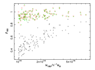
Figure 1: The ratio of the mean specific energy (thermal plus kinetic) of all particles to the gas specific energy within the virial radius for three different values of the softening: crosses, 10 $h^{-1}$kpc; circles, 50 $h^{-1}$kpc; stars, 100 $h^{-1}$kpc.

As can be seen from the Figure, the effect of using too small a softening can be severe. Putting soft=$10\,h^{-1}$kpc into Equation 3 gives $t_{r,{\rm min}}/t_{0}\approx$0.12–0.24 for the lowest-to-highest mass clusters shown in the Figure. The Steinmetz & White criterion makes only a very slight distinction between the three runs with different softening (which enters Equation 4 only via the Coulomb logarithm) and so should be regarded as a necessary but not sufficient condition to prevent artificial heating.

Figure 2 shows the profile of $\beta$ as a function of radius (i.e. $\beta(r)$ is the ratio of the mean specific energy of all particles to the mean specific energy of gas particles within spherical shells about the cluster centre). Because individual profiles show large variations in $\beta$, we have averaged the profiles of the 70-80 smallest clusters, $M<2\times 10^{14}h^{-1}$$\rm\,M_{\odot}$, that show minimal substructure ($S<0.2$: see Section 2.3)—these are the clusters with the lowest values of $t_{r,{\rm min}}/t_{0}$. There is no evidence for core heating in the runs with softenings of 50 and 100 $h^{-1}$kpc, whereas for the 10 $h^{-1}$kpc softeing run $\beta$ is suppressed not only in the core but throughout the cluster. This suggests that much of the heating is going on in sub-halos before the cluster forms. As the properties of these sub-halos are similar to those of the final cluster core, this would explain why the Thomas & Couchman formula (Equation 3) is more appropriate than that of Steinmetz & White (Equation 4).

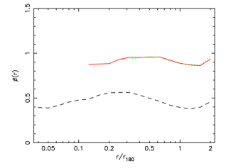
Figure 2: The ratio of the mean specific energy (thermal plus kinetic) to the gas specific energy as a function of radius for the 70-80 lowest-mass clusters that have minimal substructure, in the 112.9$\,h^{-1}$Mpc simulations. The dashed, solid and dotted lines are for softenings of 10, 50 and 100$\,h^{-1}$kpc, respectively.

It is clear from Figures 1 and 2, that there is little difference between the results for softenings of 50 and 100 $h^{-1}$kpc. They have similar values of $\beta_{180}$ and the radial variation in $\beta$ is minimal. We conclude that a softening of 50 $h^{-1}$kpc is adequate for our purposes.

The softenings for each of the other two boxes were chosen to give a similar central value of $t_{r,{\rm min}}/t_{0}$ for the lowest-mass clusters as in the 50 $h^{-1}$kpc softening run. The values of $\beta_{180}$ for each of the three production simulations are shown in Figure 3. Clusters with significant substructure, $S>0.2$, are shown as open symbols; smooth clusters with solid symbols. In this figure and all those that follow, clusters from the simulations of side 50.0, 112.9 and 153.0 $h^{-1}$Mpc are shown as triangular, circular and square symbols, respectively.

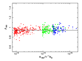
Figure 3: The ratio of the gas specific energy (thermal plus kinetic) to the dark matter specific energy within the virial radius for all clusters. In this and subsequent figures, clusters extracted from the 50, 112.9 and 153 $h^{-1}$Mpc boxes are plotted using triangular, circular and square symbols, respectively. The 14 percent of the clusters with $S>0.2$ are plotted with open symbols; the others with solid symbols. The best fit constant is show by the solid line.

Navarro & White (1993) and Pearce, Thomas & Couchman (1994) have shown that gas can gain energy from dark-matter during gravitational collapse even in the absence of numerical heating. The mechanism is quite straight-forward: both the gas and dark matter are stirred during the collapse, however the gas is able to thermalise its kinetic energy, then pick up more at the expense of the dark matter. There is no reason to suppose that this process should have occurred equally in low- and high-mass clusters. There are hints of a slight decline in $\beta_{180}$ at low masses in Figure 3, but to a good approximation, $\beta_{180}$ is independent of mass and equal to 0.94$\pm 0.03$. Thus the fractional heating is comparable to, but slightly smaller than, the estimate of 10 per cent that we made from the Steinmetz & White formula.

Because the gas has a greater specific energy than the dark matter, it is more extended and hence the baryon fraction within the virial radius is smaller than the global average. We measure it to be approximately $(0.85\pm 0.02)\,\Omega_{b}$ in our simulated clusters, independent of mass.

3 Cluster profiles

In clusters, the dark matter is dynamically dominant. It is therefore important to have a good model of the dark-matter mass distribution. Navarro, Frenk & White (1995, 1996, 1997) showed that the density profiles of simulated clusters in a wide variety of cosmological models are well-described by the formula

$$\rho={\rho_{0}\over x\,(1+x)^{2}},$$ (5)

where $r=ax$ is the radius and $\rho_{0}$ and $a$ are free parameters, and went so far as to describe this as a ‘universal density profile’. This formula must break down at large radii as it predicts infinite mass, but it appears to hold out to the virial radius, defined (in critical-density models) as the radius, $r_{180}$, enclosing a mean overdensity of 180.

In a previous paper Thomas et al. (1998) found that the NFW formula was indeed a good approximation to the mass distribution of an average cluster, but that there was a wide dispersion in the rate at which the density was declining at the virial radius. Hence we introduce a more general profile

$$\rho={\rho_{0}\over x\,(1+x)^{s}},$$ (6)

where $s$ is a constant. Because the name is now so well-established in the literature, we call this the ‘generalised NFW’ model, although we note that the case $s=3$ was introduced first, by Hernquist (1990).

The resolution of the simulations presented in this paper is not sufficient to determine the density profile in the cores of the clusters. This has been looked at in depth by Moore et al. (1998) and by Jing & Suto (2000). There is now evidence to suggest that the inner density cusp rises more steeply than $\rho\propto r^{-1}$, but that is of little consequence for the overall dynamics of the cluster and so we will stick with Equation 6 here.

3.1 Best-fit circular speed profiles

The density profiles of individual clusters are often very noisy which makes them difficult to match to any given theoretical profile. It is better to use a cumulative profile such as the circular speed, $v_{\rm c}$, which is anyway a dynamically more relevant quantity. For the above distribution,

$$v_{\rm c}^{2}\propto{(1+x)^{s-1}-(s-1)\,x-1\over x\,(1+x)^{s-1}}$$ (7)

when $s\neq 2$, and

$$v_{\rm c}^{2}\propto{(1+x)\ln(1+x)-x\over x\,(1+x)}$$ (8)

when $s=2$.

An example of a circular-speed profile is given in Figure 4 together with the best-fit function of the form of Equation 7. We have fitted and plotted the curve between twice the softening and twice the virial radius. This particular cluster was chosen because the goodness-of-fit as measured by the mean-square deviation from the theoretical curve is the median value for all the clusters. As can be seen, there are kinks in the profile, showing evidence of substructure: this is typical of most of the clusters in our catalogue.

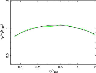
Figure 4: The circular-speed profile for one of the clusters. The best-fit theoretical model is shown by the smooth curve.

The best-fit values of $s$ as a function of cluster mass are shown in Figure 5. Note that $s$ has been limited to be less than or equal to 10.

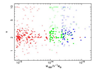
Figure 5: $s$ versus $M_{180}$ for all the clusters. The solid symbols represent clusters for which the slope of the density profile at two virial radii is within 25 per cent of the asymptotic slope at large radii.

The asymptotic density profile at large radii has a slope of $-(s+1)$. However, this is not always representative of the slope at two virial radii, the outer radius to which we fit the rotation curve. Hence we plot with solid symbols in the Figure only those clusters for which the two differ by less than $0.2s$—this corresponds to a characteristic radius $a<0.5r_{180}$.

A quick glance at Figure 5 makes the suggestion that $s=2$ is a universal density profile seem surprising. However, it is hard to measure the density profiles in the outer parts of clusters with any degree of accuracy and the answer that one gets often depends upon the radial extent of the fit. At one virial radius, the slope of the density profile is far from $-(s+1)$ and so the asymptotic slope is poorly constained. In addition, $s$ and $a$ are strongly correlated and it is often possible to get a reasonable fit by forcing $s=2$ and allowing $a$ to vary. Hence the statement that the profile within one virial radius is ‘consistent with and NFW profile’ is largely meaningless. It is for this reason that we choose to fit the profile within two virial radii instead.

We define clusters to be consistent with an NFW profile if the asymptotic slope of their density profile lies between $-2.8$ and $-3.2$ (i.e. $1.8<s<2.2$). Just under a quarter of the clusters meet this criterion.

The best-fit profiles of many clusters plotted with open symbols show a high value of $s$. However, this does not indicate steep density profiles at large radii because the best-fit core radii rise to compensate. Rather, it indicates that the functional form of the generalised NFW profile is a poor representation of the cluster. As an example consider the cluster shown in Figure 6.

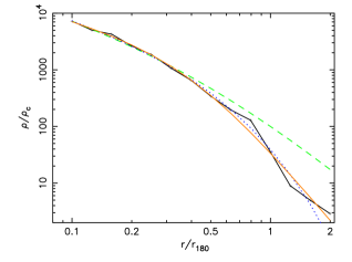
Figure 6: The density profile for one of the clusters. The dashed line shows the best-fit NFW model. The dotted line shows the best-fit generalised NFW model with $s=10$. The solid line shows a better, alternative model, as described in the text.

This is a smooth cluster: visually it appears spherically-symmetric and its substructure parameter is small, $S=0.038$. In addition, the best-fitting ellipsoid (see Thomas et al. 1998) is amongst the most spherical of any cluster with axial ratios of 1.14:1.0:0.94. However, the density profile, even out to 0.8 virial radii, is poorly fit by an NFW profile (dashed line). Also, it shows a sharp change in slope at this radius that cannot be matched by any generalised NFW profile. The dotted line shows a generalised NFW model with $s=10.$ and $a=3.1\,r_{180}$. In order to reproduce the sharp decline in density at the virial radius, $s$ has to be very large, but this then leads to a density profile that is declining far too rapidly in the outer parts of the cluster (and would steepen even more at radii larger than those shown in the Figure). A better representation of the density profile in this case is given by the dotted line which corresponds to the function

$$\rho={\rho_{0}\over x\,(1+x^{2})^{s/2}},$$ (9)

where $x=r/a$ as before, and $s=3.2$, $a=0.40\,r_{180}$. This value of $s$ is a much better estimate of the asymptotic slope of the density profile at large radii.

It can be seen from Figure 5 that the line $s=3$ roughly separates the solid from the open symbols in the upper half of the plot. Thus, where the outer slope of the density profile is well-defined, it generally lies between $-3$ (an NFW profile) and $-4$ (a Hernquist profile). The open symbols represent clusters, like that shown in Figure 6, that have a sharper break in their density profile than can be fit by a generalised NFW profile: these comprise about 30 per cent of the total cluster sample.

The open symbols that correspond to values of $s$ less than 2 are mostly clusters that show some degree of substructure, for which the density profile is not well-defined. These comprise another 16 percent of the cluster population.

Although the spread in $s$ is large, there is a weak trend for $s$ to increase with mass. To make this more evident, we define an average low-mass and an average high-mass cluster by selecting all relatively smooth clusters, $S<0.2$, in the mass ranges $M<1.2\times 10^{13}h^{-1}$$\rm\,M_{\odot}$and $M>3.0\times 10^{14}h^{-1}$$\rm\,M_{\odot}$. The resulting profiles are extremely well-fit by our theoretical model with slopes of $s=2.0$ and $s=2.3$, respectively.

It is clear from the above analysis that there is no ‘universal profile’ for dark matter halos. A substantial proportion of clusters show obvious substructure, and even those that don’t exhibit a wide variety of functional forms for the spherically-averaged density profiles of halos.

3.2 Best-fit NFW profiles and concentrations

The concept of a universal density profile is an attractive one. It makes modelling of observed clusters much simpler and it has the advantage that there is only one free parameter—the ratio of the characteristic radius in the NFW formula to the virial radius, $x_{180}=r_{180}/a(s=2)$. Therefore, we wish to see how well one can approximate cluster properties by assuming that they all follow the NFW profile, in defiance of the results of Section 3.1.

The best-fit values of $x_{180}$ as a function of mass are shown in Figure 7. There is a general trend of decreasing concentration as one moves to higher masses, but once again the scatter is large. The solid line in Figure 7 corresponds to the function

$$x_{180}=3.7\,\left(M\over 10^{15}h^{-1}\hbox{$\rm\,M_{\odot}$}\right)^{-0.1}.$$ (10)

The 86 per cent of the clusters with $S<0.2$ are spread equally above and below the line. We shall use this relation in the analysis that follows to see how well the simple NFW model predicts the measured scaling relations between temperature and mass.

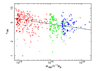
Figure 7: The measured concentration assuming an NFW profile, $x_{180}$, versus mass within the virial radius, $M_{180}$, for all the clusters. The 14 percent of the clusters with $S>0.2$ are plotted with open symbols; the others with solid symbols.

We can compare our concentration parameters to those of Navarro, Frenk & White (1997), by measuring halo mass in terms of $M_{*}$, the mass of a spherical region with root-mean-square linear density fluctuation of 1.69 today. For our simulations, $M_{*}\approx 3.3\times 10^{12}h^{-1}\hbox{$\rm\,M_{\odot}$}$, and $M_{180}/M_{*}$ ranges from 3 to 300. This gives concentrations in good agreement with their CDM models.

Interestingly, Figure 8 shows that the measured concentrations are highly-correlated with the substructure statistic. Thus low concentrations do not normally occur in spherically-symmetric clusters, but come from spherical averaging of clusters that have substructure. This suggests that the weak trend of decreasing concentration with increasing mass is driven primarily by the fact that substructure increases with mass, as shown in Figure 9.

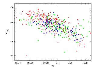
Figure 8: $x_{180}$ versus $S$ for all the clusters. Note that six points to the left and the bottom of this plot have been omitted for clarity.

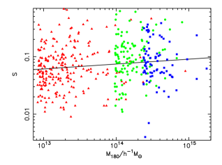
Figure 9: $S$ versus $M_{180}$ for all the clusters. A couple of points have been omitted from the bottom of the plot, for clarity. The solid line shows a median line that divides both the triangles and the circles plus squares into two equal groups.

We conclude this section by plotting in Figure 10 the temperature profiles for the mean clusters described above. The lower curve in each panel shows the gas temperature in units of keV$/k$, while the upper curve shows the total specific energy of the gas (thermal plus kinetic) in the same units. It should be noted that the gas is approximately isothermal within about one-third of the virial radius, but that its temperature drops rapidly in the outer parts of the cluster. This is a reflection of the fact that the specific energy of the dark matter declines in the outer regions of the cluster, because the ratio between the two is approximately constant out to two virial radii.

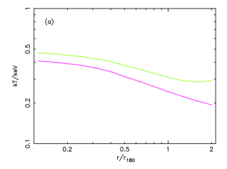
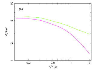
Figure 10: Mean temperature profiles for (a) 79 low-mass, and (b) 34 high-mass clusters, as described in the text. The upper curve in each case shows the total specific energy of the gas and the lower curve the temperature, both in units of keV/k.

It is a matter of some debate in the literature as to whether the observed temperature profiles of clusters are isothermal or decline to large radii. Using ASCA data, Irwin & Bregman (2000) and White (2000) infer flat or slowly increasing temperature profiles within 0.3 $r_{\rm 180}$, whereas Markevitch et al. (1998) find that the temperature drops by a factor of two within 0.5 $r_{180}$. It is clear from our simulations that isothermal profiles beyond about 0.3 $r_{\rm 180}$ are inconsistent with our simple model and would probably require some form of non-gravitational heating.

4 Predicted scaling relations

In this section, we predict scaling relations for model clusters under the assumptions that they are spherically-symmetric, isolated and in hydrodynamical equilibrium. It is not that we are asserting that these assumptions are true, but rather we want to see how well such a simple model will perform and to test the sensitivity of the scaling relations to changes in the model parameters.

By scaling everything in terms of a characteristic radius, $a$, and density $\rho_{0}$, for each cluster, we can make all the variables dimensionless. We write $r=ax$ and $\rho=\rho_{0}\tilde{\rho}$, where

$$\tilde{\rho}={1\over x\,(1+x)^{s}}.$$ (11)

and the tilde indicates a dimensionless quantity. Similarly, for the mass within radius $r$,

$$m=4\pi\rho_{0}\,a^{3}\tilde{m}$$ (12)

where

$$\tilde{m}=\int_{0}^{r/a}\tilde{\rho}\,x^{2}\mbox{d}x.$$ (13)

When we observe clusters, we usually measure their properties at or within the virial radius, $r_{\rm vir}=a\,x_{\Delta_{c}}$ at which their enclosed density equals some multiple, $\Delta_{c}$, of the critical density of the universe. For the $\tau$CDM model that we consider in this paper, $\Delta_{c}=180$, but we will set $r_{\delta}=a\,x_{\delta}$ and leave $\delta$ as a free parameter, so as to be completely general in our argument.

From the above definitions, we can write $\rho_{0}$ in terms of $x_{\delta}$,

$$\rho_{0}=60\,\delta_{180}\,\rho_{c}\,{x_{\delta}^{3}\over\tilde{m}_{\delta}},$$ (14)

where $\rho_{c}$ is the critical density, $\delta_{180}=\delta/180$ and $\tilde{m}_{\delta}=\tilde{m}(x_{\delta})$.

4.1 The virial temperature-mass relation

We next calculate the velocity dispersion, $\sigma$ as a function of radius for the NFW profile. To do this, we assume that the velocity ellipsoid is isotropic. It then becomes convenient to write $\sigma^{2}=kT/\mu m_{H}$, where $k$ is the Boltzmann constant, $\mu m_{H}$ is the mean particle mass for the gas, and $T$ is the ‘dynamical temperature’ of the halo. If the specific energy of the gas and dark-matter were the same, then $T$ would be equal to the gas temperature.

The spherically-symmetric Jeans’ Equation for a fluid with an isotropic velocity dispersion is

$${\mbox{d}(\tilde{\rho}\tilde{T})\over\mbox{d}x}=-{\tilde{m}\tilde{\rho}\over x^{2}},$$ (15)

where

$$T={G\mu m_{H}\over k}\,4\pi\rho_{0}a^{2}\,\tilde{T}.$$ (16)

We are now in a position to calculate the mean dynamical temperature, $T_{\delta}$, within radius $r_{\delta}$. By definition,

$$\tilde{m}_{\delta}\,\tilde{T}_{\delta}=\int_{0}^{\tilde{m}_{\delta}}\tilde{T}\,\mbox{d}\tilde{m}=\int_{0}^{x_{\delta}}\tilde{\rho}\,\tilde{T}\,x^{2}\mbox{d}{x}.$$ (17)

Combining Equations 12 and 16 to eliminate $a$, and then substituting for $\rho_{0}$ from Equation 14, gives

$$k\,T_{\delta} = G\mu m_{H}\,(240\pi\rho_{c}\,\delta_{180})^{1\over 3}\,{x_{\delta}\,\tilde{T}_{\delta}\over\tilde{m}_{\delta}}\,m_{\delta}^{2\over 3}$$ (18)

$$\approx 16.0\,\delta_{180}^{1\over 3}\,{x_{\delta}\,\tilde{T}_{\delta}\over\tilde{m}_{\delta}}\,\left(m_{\delta}\over 10^{15}h^{-1}\hbox{$\rm\,M_{\odot}$}\right)^{2\over 3}\hbox{keV},$$

where we have taken $\mu m_{H}\approx 10^{-27}$kg, corresponding to a fully-ionized cosmic mix of elements.

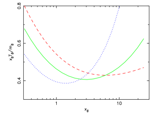
Figure 11: The shape factor $x_{\delta}\,\tilde{T}_{\delta}/\tilde{m}_{\delta}$ in the dynamical temperature-mass relation of Equation 18. The dashed, solid and dotted lines correspond to $s=1.5$, 2 and 3, respectively.

When $\delta=\Delta_{c}$, then $T_{\delta}$ is the ‘virial temperature’. We will use the notation $T_{180}$ rather than $T_{\rm vir}$, to make explicit that we are referring to an overdensity of 180 (as in other cosmologies, the virial radius would correspond to a different overdensity).

If all clusters are self-similar (e.g. if they all follow the NFW model), and if we measure the total mass, $m_{\delta}$, and mean dynamical temperature, $T_{\delta}$, within $r_{\delta}$, then it is often assumed that they must obey the relation $T_{\delta}\propto m_{\delta}^{2/3}$. This is not strictly true, however, because of the presence of the $x_{\delta}\tilde{T}_{\delta}/\tilde{m}_{\delta}$ term which varies with concentration, $x_{\delta}$.

We show the variation of $x_{\delta}\,\tilde{T}_{\delta}/\tilde{m}_{\delta}$ with $x_{\delta}$ in Figure 11 for values of $s=1.5$, 2 and 3. We see that for values of $x_{180}$ in the range 1.5 to 10 that are typical when fitting the NFW profile to clusters, $x_{180}\,\tilde{T}_{180}/\tilde{m}_{180}$ lies in the narrow range 0.4–0.47. Fitting $s=1.5$ profiles instead would give smaller values of $x_{180}$, and fitting $s=3$ profiles larger values, so that these too give approximately the same answer. Thus the virial temperature-mass relation is robust to variations in the density profile.

4.2 The gas density profile and the X-ray temperature-mass relation

The virial temperature-mass relation predicted above is of little use observationally. Instead we need to use the emission-weighted, X-ray temperature. Previous studies such as Eke, Navarro & Frenk (1998) and Makino, Susaki & Suto (1998) have calculated the mean X-ray temperature and the luminosity of the intracluster medium assuming that it is isothermal and sitting in an NFW potential. Figure 10 shows that the gas is far from isothermal and so we instead make the assumption, as indicated by Figure 2, that the ratio of the specific energies of the gas and dark matter is everywhere constant and equal to $\beta=0.94$, i.e. $T_{\rm gas}=T/\beta$.

We will further assume that the dark matter is dynamically dominant. Then

$${1\over\tilde{\rho}_{\rm gas}}\,{\mbox{d}(\tilde{\rho}_{\rm gas}\tilde{T}_{\rm gas})\over\mbox{d}x}={1\over\tilde{\rho}}\,{\mbox{d}(\tilde{\rho}\,\tilde{T})\over\mbox{d}x},$$ (19)

which can be expanded to give

$${\mbox{d}\ln\tilde{\rho}_{\rm gas}\over\mbox{d}\ln x}={\mbox{d}\ln\tilde{\rho}\over\mbox{d}\ln x}-(1-\beta)\,{\mbox{d}\ln\tilde{P}\over\mbox{d}\ln x},$$ (20)

where $\tilde{P}=\tilde{\rho}\tilde{T}$. This shows that the gas is able to support itself more effectively and hence has a shallower density gradient than the dark matter. For $\beta=0.94$, the asymptotic density gradient at large radii is $-2.7$, compared to $-3$ for the dark matter.

The mean X-ray temperature within radius $r_{\delta}$ is defined by

$$\tilde{L}_{\delta}\,\tilde{T}_{X,\delta}=\int_{0}^{\tilde{L}_{\delta}}\tilde{T}_{\rm gas}\,\mbox{d}\tilde{L},$$ (21)

where

$$\tilde{L}(x)=\int_{0}^{x}\tilde{\rho}_{\rm gas}^{2}\,\tilde{T}_{\rm gas}^{1\over 2}\,\mbox{d}x$$ (22)

and $\tilde{L}_{\delta}=\tilde{L}(x_{\delta})$. Note that we have assumed that the emissivity of the gas scales as $\tilde{T}_{\rm gas}^{1/2}$, although this is only really true at high temperatures where bremsstrahlung dominates. However, the dominant contribution to the variation in the integrand in Equation 22 comes from $\tilde{\rho}_{\rm gas}$ and so this is a reasonable approximation.

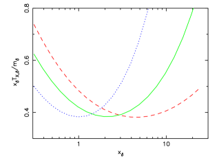
Figure 12: The shape factor $x_{\delta}\,\tilde{T}_{X,\delta}/\tilde{m}_{\delta}$ in the X-ray temperature-mass relation. The dashed, solid and dotted lines correspond to $s=1.5$, 2 and 3, respectively.

The values of the normalisation factor in the X-ray temperature-mass relation, $x_{\delta}\,\tilde{T}_{X,\delta}/\tilde{m}_{\delta}$, are shown in Figure 12. They can be seen to rise more steeply at large concentrations than in Figure 11. This is because the X-ray temperature declines far less steeply with radius than the dynamical one used previously. Figure 12 suggests that the range of concentrations seen in our simulated clusters will add quite a lot of scatter to the mean X-ray temperatures within the virial radius, with the more concentrated clusters being hotter than the less-concentrated ones for a given mass by up to 40 per cent.

5 Measured scaling relations

5.1 The virial temperature-mass relation

The location of each of our clusters on the $T_{180}$-$m_{180}$ plane is shown in Figure 13. Also shown by the dashed line is the best-fit power-law

$$k\,T_{180}\approx 6.9\,\left(m_{180}\over 10^{15}h^{-1}\hbox{$\rm\,M_{\odot}$}\right)^{0.67\pm 0.02}\hbox{keV},$$ (23)

which corresponds to a value of $x_{\delta}\tilde{T}_{\delta}/\tilde{m}_{\delta}=0.43$.

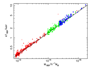
Figure 13: $T_{180}$ versus $M_{180}$ for all the clusters. In this and subsequent figures in this section, the 14 per cent of clusters that have a substructure statistic $S>0.2$ are plotted with open symbols; others as filled symbols. The dashed line shows the best-fit power-law. The solid line shows the prediction from the isotropic NFW model.

The predicted relation from Equation 18, using the median concentrations, $x_{180}$, taken from Equation 10, is shown by the solid line in the Figure. It can be seen that this predicts temperatures that are slightly too low, although the spread in temperatures is consistent with the spread in $x_{180}$ seen in Figure 7.

It would be possible to reconcile the predicted and measured relations by using slightly larger values of $x_{180}$: Figure 8 shows that the most regular clusters are biased towards higher concentrations. An alternative explanation for the low virial temperatures is that the dark matter velocity ellipsoid is not isotropic, as radial orbits are less efficient at supporting the particles within a given potential than transverse ones. This is discussed further in Section 6.2.

5.2 X-ray versus virial temperatures

The ratios of the dynamical temperatures to the X-ray temperatures, averaged within the virial radii, are shown in Figure 14.

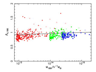
Figure 14: The ratio of the dynamical temperature to the X-ray temperature within the virial radius for all clusters. The prediction from the isotropic NFW model is show by the solid line.

The prediction from the isotropic NFW model with concentrations given by Equation 10 is shown by the solid line. It can be seen that the theoretical curve mimics the data in that it predicts that low-mass clusters should have lower values of $\beta_{X,180}$ than high-mass ones. However the mean measured values of $\beta_{X,180}$ lie about 0.1 below the predictions. Once again, this could be reconciled by using higher values of $x_{180}$ or an anisotropic dark matter velocity ellipsoid.

Although virial temperatures are notoriously difficult to measure, there is empirical evidence that the observed, X-ray temperatures of the intracluster medium are greater than the virial temperatures (e.g. Edge & Stewart 1991a,b; Bahcall & Lubin 1994). The latter give a value of $\beta_{X,180}=0.94$ for the highest-mass clusters, which is not too dissimilar from the values that we find in Figure 14. However, the results of the next section suggest values that are lower than this.

5.3 X-ray temperature-mass relations within a fixed overdensity

The relationship between X-ray temperature and mass within the virial radius is shown in Figure 15. The dashed line shows the best-fit relation from Evrard, Metzler & Navarro (1996, hereafter EMN),

$$k\,T_{X,180}\approx 7.85\,\left(m_{180}\over 10^{15}h^{-1}\hbox{$\rm\,M_{\odot}$}\right)^{0.67\pm 0.02}\hbox{keV}.$$ (24)

They extracted 58 clusters in the temperature range 1–10 keV, from three different sets of cosmological simulations with a variety of cosmological parameters. We have used the information given in their paper to interpolate their results to an overdensity of 180—our results are in good agreement.

The temperature normalisation is slightly higher than for the dynamical temperature-mass relation and corresponds to $x_{\delta}\tilde{T}_{\delta}/\tilde{m}_{\delta}=0.49$. The prediction from Equation 18 using values of $x_{180}$ taken from Equation 10 is shown by the solid line on the Figure. Once again it gives temperatures that are slightly too low.

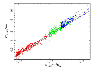
Figure 15: The X-ray temperature versus mass within the virial radius. The dashed line shows the best-fit power law; the dotted line shows the best observational results from Horner, Mushotzky & Scharf (1999) and the solid line shows the prediction from the isotropic NFW model.

The most extensive observational investigation of the $T_{X}$-$M_{\rm 180}$ relation is by Horner, Mushotzky & Scharf (1999) who used many different ways to determine the mass within the virial radius. Their preferred measure, based on X-ray emissivity and temperature profiles, gives $T_{X}\propto M_{\rm 180}^{2/3}$, while those obtained from the isothermal $\beta$-model and X-ray surface brightness deprojections are flatter, $T_{X}\propto M_{\rm 180}^{0.5-0.56}$. They suggest that the slopes of these latter two measures are too low because they assume a dark matter density profile of ${\rho_{\rm dark}\propto r^{-2}}$ whilst observations and simulations suggest that it is steeper, ${\rho_{\rm dark}\propto r^{-2.4}}$.

The preferred relation from Horner, Mushotzky & Scharf (1999) is shown as a dotted line in Figure 15. From this it is clear that either the measured cluster masses are too low, or more likely dissipationless simulations predict X-ray temperatures that are smaller than the observed values. If we combine the results from Figures 14 and 15 then this argues that observed high-mass clusters have values of $\beta_{X,180}\approx 2/3$.

This high value of $\beta_{X,180}$ might be thought to provide evidence for heating of the intracluster medium, but in fact radiative cooling can have the same effect! Pearce et al. (2000) have shown that the removal of low-entropy gas by cooling in the core of the cluster can raise the X-ray temperature of the cluster by 20 to 40 percent. This cooling is relatively more important in low-mass clusters and so would have the effect of flattening the $T_{X}$-$M$ relation slightly.

Mohr, Mathiesen & Evrard (1999) find in a sample of 45 clusters that the ICM is more extended than the dark-matter and that $T_{X}\mathrel{\hbox to0.0pt{\lower 3.0pt\hbox{$\sim$}\hss}\raise 2.0pt\hbox{$\propto$}}M_{\rm gas}^{1/2}$. In our simulations, we also find that the gas is more extended than the dark matter, due to its higher specific energy. However, the baryon fraction within the virial radius is approximately 0.85, independent of mass, and so obtain a temperature-gas mass relation that parallels the one for the total mass, $T_{X}\mathrel{\hbox to0.0pt{\lower 3.0pt\hbox{$\sim$}\hss}\raise 2.0pt\hbox{$\propto$}}M_{\rm gas}^{0.67}$. Physical processes such as heating or radiative cooling are once again required (and act in the correct sense) to reconcile the observations and simulations.

In Figure 16, we show a similar plot to Figure 15, but for the X-ray temperature-mass relation within an overdensity contour of 1000.

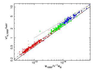
Figure 16: The X-ray temperature versus mass within a spherical shell enclosing an overdensity of 1000. The dashed line shows the best-fit power law, the dotted line shows the observational results from Nevalainen, Markevitch & Forman (2000), and the solid line shows the prediction from the isotropic NFW model.

Once again, the isotropic NFW model slightly underpredicts the X-ray temperatures (but agrees with the results of EMN). The best-fit power law is consistent with the self-similar prediction

$$k\,T_{X,1000}\approx 13.0\,\left(m_{1000}\over 10^{15}h^{-1}\hbox{$\rm\,M_{\odot}$}\right)^{0.67}\hbox{keV}.$$ (25)

The dotted line shows the observational results from Nevalainen, Markevitch & Forman (2000). The observed temperatures are again higher than the predictions from this non-radiative model but in a way that is now mass-dependent—this is consistent with our expectation that the effects of cooling and/or heating would be greater in lower-mass clusters.

5.4 The X-ray temperature-virial radius relation

From an observational point of view, it is much easier to measure the virial radius rather than the virial mass, and so it is surprising that more authors do not report the former. There is no extra information here, however, as the two are simply related and so it is possible to rewrite Equations 24 and 25 in terms of virial radius and X-ray temperature:

$$r_{180}\approx 1.9\,\left(k\,T_{X,180}\over 10\,\mbox{keV}\right)^{1\over 2}\,h^{-1}\mbox{Mpc},$$ (26)

$$r_{1000}\approx 0.85\,\left(k\,T_{X,1000}\over 10\,\mbox{keV}\right)^{1\over 2}\,h^{-1}\mbox{Mpc}.$$ (27)

These follow with the self-similar form in that they have slopes of ${1\over 2}$. $r_{180}$ agrees with the results of EMN; $r_{1000}$ has a slightly lower normalisation.

We note that the only observational measurement of $r_{1000}$ by Vikhlinin, Forman & Jones (1999) is at first sight in gross disagreement with our prediction. They have

$$r_{1000}\approx 0.415\,\left(k\,T_{X,1000}\over 10\,\mbox{keV}\right)^{0.57}\,h^{-1}\mbox{Mpc}$$ (28)

which gives a value at 5 keV of 1.04 $h^{-1}$Mpc—far in excess of the simulation results. The reason for this discrepancy is that Vikhlinin et al. have defined overdensity with respect to a mean baryon abundance of $\Omega_{b}h^{2}=0.010$ which is much lower than either recent determination from primordial nucleosynthesis ($\Omega_{b}h^{2}=0.019$, Tytler et al. 2000) or from X-ray measurements of the baryon fraction ($\Omega_{b}h^{2}=0.0594h^{1/2}$, Ettori & Fabian 1999). We can turn the argument around and ask what baryon abundance would make our results compatible with Vikhlinin et al.. The radii they quote enclose a baryon overdensity of about 230 in our models. Hence we require

$$\Omega_{b}h^{2}\approx 0.010\,{1000\over 230}\approx 0.043,$$ (29)

This agrees with the value from Etorri & Fabian for $h=0.54$.

5.5 Temperature-mass relations within the Abell radius

If we measure cluster properties within a fixed radius, rather than a fixed overdensity, then the deviation from the self-similar scaling relations can be quite large. This is shown in Figure 17 where we plot, for within the Abell radius, emission-weighted temperature versus mass. The best-fit power law, shown as the dashed line, has a slope of 0.81.

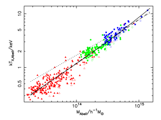
Figure 17: X-ray temperature versus mass, for properties averaged within the Abell radius, for all the clusters. The dashed line shows the best-fit power law. The dotted line is the relation from Equation 24 for properties averaged within the virial radius. The solid line shows the corrected relation as described in the text.

The reason for the steeper slope is that, for low-mass clusters, the Abell radius is greater than the virial radius and so we are averaging properties over a larger volume than before. This has the effect of lowering the X-ray temperature slightly (because the X-ray temperature is heavily weighted by emission from the centre of the cluster this effect is small), but greatly increasing the mass. For high-mass clusters, however, the virial radii are similar to the Abell radii and so there is no change.

Because the X-ray temperatures are almost unaltered, the mass-temperature relation can be estimated by simply multiplying the right-hand-side of Equation 24 by the ratio of the mass within an Abell radius to that within the virial radius, $M_{\rm Abell}/M_{180}$. We have done this, using Equation 26 to estimate the virial radii and assuming that the mass profile follows the NFW model. The result, shown as the solid line in Figure 17, closely follows the data points.

Figure 18 is the same as for Figure 17, but for properties averaged within half an Abell radius. Once again the best-fit power law has a slope, 0.86, that is steeper than the self-similar relation, and the corrected NFW model provides an excellent fit to the data.

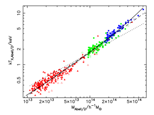
Figure 18: X-ray temperature versus mass, for properties averaged within half the Abell radius, for all the clusters. The dashed line shows the best-fit power law. The dotted line is the relation from Equation 24 for properties averaged within the virial radius. The solid line shows the corrected relation as described in the text.

6 Discussion

6.1 Comparison with previous simulations

Previous authors have also looked at scaling relations in simulations of clusters without radiative cooling. All agree that the gas is more extended than the dark matter, but disagree on the details of the $T_{X}$-$M$ relation. The studies split into two types: those that simulate a small number of clusters in detail, and those that, like us, look at a large number of clusters at moderate resolution.

Navarro, Frenk & White (1995) simulate only 6 clusters, extracted from a low-resolution simulation, but choose these to span a factor of thirty in mass and adjust the particle mass so that each cluster contains several thousand particles within the virial radius. They find a $T_{X}$-$M$ relation in agreement with the virial relation and values of $\beta$ of about unity (where their $\beta$, as ours, includes a contribution from unthermalised motions in the gas) with no dependence upon mass.

EMN have taken the Navarro, Frenk & White results and compared them with two other sets of simulations of isolated clusters from Metzler (1995) and Mohr et al. (1995). These span a range of cosmologies and use two distinct codes, yet yield very similar results. It should be noted that EMN do not quote results for an overdensity of 180, but they give sufficient information in their paper to allow one to interpolate from their preferred overdensity of 500. Once we do so, we find a $T_{X}$-$M$ relation essentially identical to ours.

Eke, Navarro & Frenk (1998) perform a similar study for 10 clusters in a $\Lambda$-CDM cosmology, ranging over a factor of only three in mass. Their results are consistent with the scaling relations but cover too small a dynamic range to provide a strong constraint.

By contrast, Bryan & Norman (1998) use a smaller box and simulate a large number of clusters at relatively poor resolution. They find that $\beta$ is an increasing function of cluster mass which suggests that numerical heating is having an effect. They also find a $T_{X}$-$M$ relation that is flatter than the self-similar one, but only for an open cosmology.

Yoshikawa, Jing & Suto (2000) have undertaken similar simulations to ourselves, but with a poorer spatial resolution and covering a smaller mass-range. They too find the expected slope of ${2\over 3}$ for the $T_{X}$-$M$ relation.

6.2 Beyond the isotropic NFW model

It can be seen from Figures 13 and 15 that the isotropic NFW model underpredicts the virial temperature slightly and the X-ray temperature quite a lot.

One possible explanation for the low virial temperatures is that the dark matter velocity ellipsoid is not isotropic, as radial orbits are less efficient at supporting the particles within a given potential than transverse ones.

We have checked that a ratio of the transverse to radial velocity dispersion of $\sigma_{t}=0.9\,\sigma_{r}$ is sufficient to bring the dashed and solid lines in Figures 13 and 15 into close agreement. We choose not to report on this in detail, however, because we believe that it overly-complicates the simple model that we are trying to test. It should be remembered that few of our clusters are free from some form of substructure and this too would invalidate the simple NFW model.

We prefer to conclude that the isotropic NFW model does pretty well, whilst bearing in mind that it underestimates the temperatures slightly.

7 Conclusions

We extract clusters, covering more than 2 decades in mass, from three simulations of the $\tau$CDM cosmology. This represents the largest, uniform catalogue of simulated clusters ever produced.

We fit the circular-speed profiles of the clusters with models corresponding to spherically-symmetric density profiles of the form

$$\rho={\rho_{0}\over x\,(1+x)^{s}},$$ (30)

where $s=2$ corresponds to the renowned NFW profile.

We find that the scatter in the best-fit values of $s$ is large, with under a quarter of the clusters being accurately fit by the NFW model. The others either have steeper outer slopes in their density profiles, show a sharp break in their density profiles that cannot be fit by the above form, or have significant substructure. However, the mean, smooth, low-mass cluster does have $s\approx 2$, whereas the equivalent high-mass cluster has a steeper profile with $s\approx 2.8$.

When we force $s=2$, then the cluster concentrations show a large scatter, but the median concentration declines slightly with mass. This is driven primarily by an anti-correlation between concentration and substructure, with substructure being more prevalent in high-mass clusters.

We investigate how well this median NFW model predicts the cluster temperature-mass scaling relations, by deriving theoretical relationships between both dynamical and emission-weighted, X-ray temperature and mass in the isotropic NFW model, as a function of cluster concentration. The virial temperature-mass relation, averaged within a spherical region enclosing an overdensity of 180, closely mimics the self-similar form and lies a few per cent above the NFW prediction.

The gas in our clusters is hotter than the dark matter but we do not attach much significance to this: there will be a small amount of true and numerical heating due to heating by clumps and individual particles of dark matter. More importantly, we have chosen in this paper to neglect the effects of radiative cooling and heating associated with metal enrichment of the intracluster medium.

When measured within spheres enclosing a fixed overdensity, the X-ray temperature versus virial mass relation has a slope of approximately 0.67, in agreement with the self-similar prediction and with previous work (but extending over a greater mass-range). The normalisation is lower than that of the observations. This is almost certainly because we have chosen to neglect cooling and/or heating.

The radius-temperature relation is in agreement with the measured value of Vikhlinin, Forman & Jones (1999) provided that the baryon fraction is large, as indicated by Ettori & Fabian (1999).

When averaged within an Abell radius (or half an Abell radius), the X-ray temperature versus mass relation is steeper, with a slope of 0.81 (or 0.86). This is because the Abell radius is a greater multiple of the virial radius in low-mass clusters as compared to high-mass ones and so increases their measured mass.

We have not commented on the X-ray luminosity in this paper, because our simulations are not able to fully resolve the X-ray emission in the cluster cores. This core gas has a cooling time that is anyway less than the age of the Universe and so cannot be correctly modelled using a non-radiative simulation. We note that the results of Pearce et al.(2000) suggest that radiative cooling will act so as to raise the temperature of the intracluster medium and so tend to bring our simulated clusters into agreement with the observations.

In future papers we will contrast the dynamics of the gas and dark matter in clusters, consider the effect of heating and cooling processes, and compare the results from different cosmological models.

References

- [1] Bahcall N., Lubin L., 1994, ApJ, 426, 513
- [2] Bryan G. L., Norman, M. L., 1998, ApJ, 495, 80
- [3] Couchman H. M. P., Thomas P. A., Pearce F. R., 1995, MNRAS, 452, 797
- [4] Crone M. M., Evrard A. E., Richstone D. O., 1996, ApJ, 467, 489
- [5] Edge A. C., Stewart G. C., 1991a, MNRAS 252, 414
- [6] Edge A. C., Stewart G. C., 1991b, MNRAS 252, 428
- [7] Eke V. R., Cole S., Frenk C. S., 1996, MNRAS, 282, 263
- [8] Eke V. R., Cole S., Frenk C. S., Henry J. P., 1998, MNRAS, 298, 1145
- [9] Eke V. R., Navarro J. F., Frenk C. S., 1998, ApJ, 503, 569
- [10] Ettori S. & Fabian A. C., 1999, MNRAS, 305, 834
- [11] Evrard A. E., Metzler C. A., Navarro J. F., 1996, ApJ, 469, 494
- [12] Governato F., Babul A., Quinn T., Tozzi P., Baugh C. M., Katz N., Lake G., 1999, MNRAS, 307, 949
- [13] Gross M. A. K., Somerville R. S., Primack, J. R., Holtzman, J., Klypin, A., 1998, MNRAS, 301, 81
- [14] Henry J. P., 1997, ApJ, 489, L1
- [15] Hernquist L., 1990, ApJ, 356, 359
- [16] Hjorth J., Oukbir J., van Kampen, E., 1998, MNRAS, 298, L1
- [17] Horner D. J., Mushotzky R. F., Scharf C. A., 1999, ApJ, 520, 78
- [18] Irwin J. A., Bregman J. N., 2000, ApJ, submitted (astro-ph/0003123)
- [19] Jenkins A., Frenk C. S., White S. D. M., Colberg J. M., Cole S., Evrard A. E., Yoshida N., 2000, MNRAS, submitted (astro-ph/0005620)
- [20] Jing Y. P., Suto, Y., 2000, ApJ, 529, 69
- [21] Lacey C. G., Cole S., 1993, MNRAS, 262, 627
- [22] Lilje P. B., 1992, ApJ, 386, L33
- [23] Makino N., Susaki S., Suto Y., 1998, ApJ, 497, 555
- [24] Markevitch M., 1998, ApJ, 504, 27
- [25] Markevitch M., Forman W. R., Sarazin C. L., Vikhlinin A., 1998, ApJ, 503, 17
- [26] Metzler C. A., 1995, Ph.D. thesis, Univ. of Michigan
- [27] Mohr J. J., Evrard A. E., Fabricant D. G., Gheller M. J., 1995, ApJ, 447, 8
- [28] Mohr J. J., Mathiesen B., Evrard A. E., 1999, 517, 627
- [29] Moore B., Governato F., Quinn T., Stadel J., Lake, G., 1998, ApJ, 499, 5
- [30] Navarro J. F., Frenk C. S., White S. D. M., 1995, MNRAS, 275, 720
- [31] Navarro J. F., Frenk C. S., White S. D. M., 1996, ApJ, 462, 563
- [32] Navarro J. F., Frenk C. S., White S. D. M., 1997, ApJ, 490, 493
- [33] Navarro J. F., White S. D. M., 1993, MNRAS, 265, 271
- [34] Nevalainen J., Markevitch M., Forman W., 2000, ApJ, 532, 694
- [35] Pearce F. R., Couchman H. M. P., 1997, New Astron., 2, 411
- [36] Pearce F. R., Thomas P. A., Couchman H. M. P., 1994, MNRAS, 268, 953
- [37] Pearce F. R., Thomas P. A., Couchman H. M. P., Edge A. C., 2000, MNRAS, in press (astro-ph/9912013)
- [38] Press W. H., Schechter P. G., 1974, ApJ, 187, 425
- [39] Steinmetz M., White S. D. M., 1997, MNRAS, 288, 545
- [40] Thomas P. A. et al.(the Virgo Consortium), 1998, MNRAS, 296, 1061
- [41] Thomas P. A., Couchman H. M. P., 1992, MNRAS, 257, 11
- [42] Tytler D., O’Meara J. M., Suzuki N., Lubin D., 2000, PhST, 85, 12
- [43] Viana P. T. P., Liddle A. R., 1996, MNRAS, 281, 323
- [44] Viana P. T. P., Liddle A. R., 1999, MNRAS, 303, 535
- [45] Vikhlinin A, Forman W., Jones C., 1999, ApJ, 525, 47
- [46] White D. A., 2000, MNRAS, submitted (astro-ph/9909467)
- [47] Yoshikawa K., Jing Y. P., Suto Y., 2000 (astro-ph/0001076)