PARAMETER ESTIMATION IN ASTRONOMY
WITH POISSON-DISTRIBUTED DATA.
II. THE MODIFIED CHI-SQUARE-GAMMA STATISTIC

Abstract

I investigate the use of Pearson’s chi-square statistic, the Maximum Likelihood Ratio statistic for Poisson distributions, and the chi-square-gamma statistic (Mighell 1999, ApJ, 518, 380) for the determination of the goodness-of-fit between theoretical models and low-count Poisson-distributed data. I demonstrate that these statistics should not be used to determine the goodness-of-fit with data values of 10 or less.

I modify the chi-square-gamma statistic for the purpose of improving its goodness-of-fit performance. I demonstrate that the modified chi-square-gamma statistic performs (nearly) like an ideal $\chi^{2}$ statistic for the determination of goodness-of-fit with low-count data. On average, for correct (true) models, the mean value of modified chi-square-gamma statistic is equal to the number of degrees of freedom $(\nu)$ and its variance is $2\nu$ — like the $\chi^{2}$ distribution for $\nu$ degrees of freedom. Probabilities for modified chi-square-gamma goodness-of-fit values can be calculated with the incomplete gamma function.

I give a practical demonstration showing how the modified chi-square-gamma statistic can be used in experimental astrophysics by analyzing simulated X-ray observations of a weak point source (S/N$\approx 5.2\,$; 40 photons spread over 317 pixels) on a noisy background (0.06 photons per pixel). Accurate estimates (95% confidence intervals/limits) of the location and intensity of the X-ray point source are determined.

1 INTRODUCTION

The goodness-of-fit between an observation of $N$ data values, $x_{i}$, with errors, $\sigma_{i}$, and a model, $m_{i}$, can be determined by using the standard chi-square statistic:

$$\chi^{2}\equiv{\sum_{i=1}^{N}}\left[\frac{x_{i}-m_{i}}{\sigma_{i}}\right]^{2}\,.$$ (1)

The standard chi-square statistic is the appropriate statistic to determine the goodness-of-fit whenever the errors can be described by a normal (a.k.a. Gaussian) distribution.

Let us consider a more complicated situation where all the data values come from a pure counting experiment where each measurement, $n_{i}$, is a random integer deviate drawn from a Poisson (po1837 (1837), p. 205 et seq.) distribution,

$$P(k;\mu)\equiv\frac{\mu^{k}}{k!}e^{-\mu}\,,$$ (2)

with a mean value of $\mu$. The use of equation (1) in analyzing Poisson-distributed data is technically never correct. While the Poisson distribution approaches the normal distribution as the Poisson mean approaches infinity, a Poisson distribution never actually becomes a normal distribution even at very large Poisson mean values. The normal distribution is always symmetric; the coefficient of skewness for the normal distribution is zero. Poisson distributions are always asymmetric; the coefficient of skewness for a Poisson distribution of mean $\mu$ is $\mu^{-1/2}$. While the Poisson distribution is almost symmetric about the mean for large mean values, its shape becomes progressively more asymmetric as the mean approaches zero. Thus the standard assumption that a Poisson distribution is approximately normally distributed is a good approximation only when the coefficient of skewness is negligible (e.g., $\mu^{-1/2}\!\ll\!1$).

How does one then determine the goodness-of-fit with Poisson-distributed data? Historically, many $\chi^{2}$ statistics have been proposed for the analysis of Poisson-distributed data. This paper will investigate the following four:
Pearson’s $\chi^{2}$:

$$\chi_{\rm{P}}^{2}\equiv{\sum_{i=1}^{N}}\frac{(n_{i}-m_{i})^{2}}{m_{i}}\ ,$$ (3)

where the expectation value of the mean of the parent Poisson distribution of the $i$th data value is assumed to be equal to the Poisson deviate [$\langle\,\mu_{i}\,\rangle=n_{i}$] and the square of the measurement error is assumed to be equal to the mean of the model Poisson distribution [$\sigma^{2}_{i}=m_{i}$];
the modified Neyman’s $\chi^{2}$:

$$\chi_{\rm{N}}^{2}\equiv{\sum_{i=1}^{N}}\frac{(n_{i}-m_{i})^{2}}{{\rm{max}}(n_{i},1)}\ ,$$ (4)

where the expectation value of the mean of the parent Poisson distribution of the $i$th data value is assumed to be equal to the Poisson deviate [$\langle\,\mu_{i}\,\rangle=n_{i}$] and the square of the measurement error is assumed to be equal to Poisson deviate or one — whichever is greater [$\sigma^{2}_{i}={\rm{max}}(n_{i},1)$];
the Maximum Likelihood Ratio statistic for Poisson distributions:

$$\chi^{2}_{\lambda}\equiv 2{\sum_{i=1}^{N}}\left[m_{i}-n_{i}+n_{i}\ln\left(\frac{n_{i}}{m_{i}}\right)\right]$$ (5)

(see, e.g., Baker & Cousins baco1984 (1984) and references therein);
and the chi-square-gamma statistic (Mighell mi1999 (1999); hereafter PaperI):

$$\chi^{2}_{\gamma}\equiv{\sum_{i=1}^{N}}\frac{\left[n_{i}+\min\left(n_{i},1\right)-m_{i}\right]^{2}}{n_{i}+1}\ ,$$ (6)

where the expectation value of the mean of the parent Poisson distribution of the $i$th data value is assumed to be equal to the Poisson deviate plus a small correction factor of zero for zero deviates and one in all other cases [$\langle\,\mu_{i}\,\rangle=n_{i}+\min(n_{i},1)$] and the square of the measurement error is assumed to be equal to the Poisson deviate plus one [$\sigma^{2}_{i}=n_{i}+1$].

In PaperI, I demonstrated that the application of the standard weighted mean formula, $\left[\sum_{i}{n_{i}\sigma^{-2}_{i}}\right]/\left[\sum_{i}{\sigma^{-2}_{i}}\right]$, to determine the weighted mean of data, $n_{i}$, drawn from a Poisson distribution, will, on average, underestimate the true mean by $\sim$$1$ for all Poisson mean values larger than $\sim$$3$ when the common assumption is made that the error of the $i$th observation is $\sigma_{i}=\max(\sqrt{n_{i}},1)$. This small, but statistically significant offset, explains the long-known observation that chi-square minimization techniques which use the modified Neyman’s $\chi^{2}$ statistic [eq. (4)] to compare Poisson-distributed data with model values, $m_{i}$, will typically predict a total number of counts that underestimates the actual total by about $1$ count per bin (see, e.g., Bevington be1969 (1969), Wheaton et al. weet1995 (1995)).

Based on my finding that the weighted mean of data drawn from a Poisson distribution can be determined using the formula $\left[\sum_{i}\left[n_{i}+\min\left(n_{i},1\right)\right]\left(n_{i}+1\right)^{-1}\right]/\left[\sum_{i}\left(n_{i}+1\right)^{-1}\right]$, I proposed that the chi-square-gamma statistic, $\chi^{2}_{\gamma}$ [eq. (6)], should always be used to analyze Poisson-distributed data in preference to the modified Neyman’s $\chi^{2}$ statistic. Following my own advice, I will not discuss the modified Neyman’s $\chi^{2}$ statistic in the remainder of this article.

The chi-square distribution for $\nu$ degrees of freedom approaches a Gaussian distribution with a mean equal to $\nu$ (i.e., $\mu\equiv\nu$) and a variance equal to $2\nu$ (i.e., $\sigma^{2}\equiv 2\nu$) as the number of degrees of freedom approaches infinity. Ideally, a $\chi^{2}$ statistic for Poisson distributions for $\nu$ (independent) degrees of freedom would exhibit the same behavior as the number of degrees of freedom approaches infinity for all Poisson mean values (i.e., $\mu\!>\!0$).

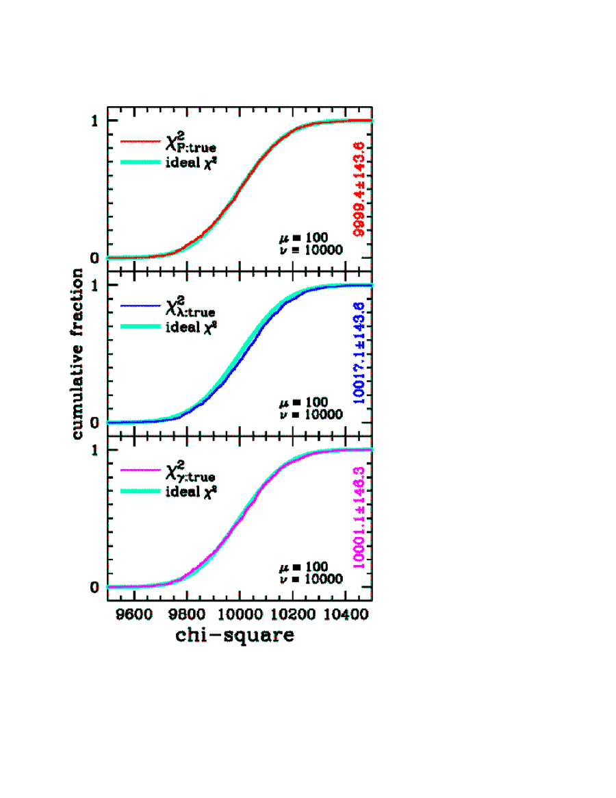
Do the $\chi^{2}_{\rm{P}}$, $\chi^{2}_{\lambda}$, and the $\chi^{2}_{\gamma}$ statistics perform as expected for large Poisson mean values? These three $\chi^{2}$ statistics are applied to the same data set in Fig. 1 (top to bottom, respectively). For this example, an ideal $\chi^{2}$ statistic for Poisson-distributed data would have a cumulative distribution similar to that of the chi-square distribution for $10^{4}$ degrees of freedom which well approximated as the cumulative distribution function of a Gaussian distribution with a mean of $10^{4}$ and a variance of $2\!\times\!10^{4}$. The results of the top and bottom panels are well matched to the expected cumulative distribution; the differences between the expected and measured mean and rms values are not statistically significant. The $\chi^{2}_{\rm{P}}$ and the $\chi^{2}_{\gamma}$ statistics perform as expected with a Poisson mean value of 100. The cumulative distribution of the middle panel, however, clearly deviates from the expected cumulative distribution; the difference between the expected and measured mean and rms values, while small, is statistically significant. The $\chi^{2}_{\lambda}$ does not perform like an ideal $\chi^{2}$ statistic for Poisson distributions with a mean value of 100 — a level that is generally considered to be well above the low-count regime ($\mu\mathrel{<\kern-10.00002pt\lower 3.87495pt\hbox{$\sim$}}25$).

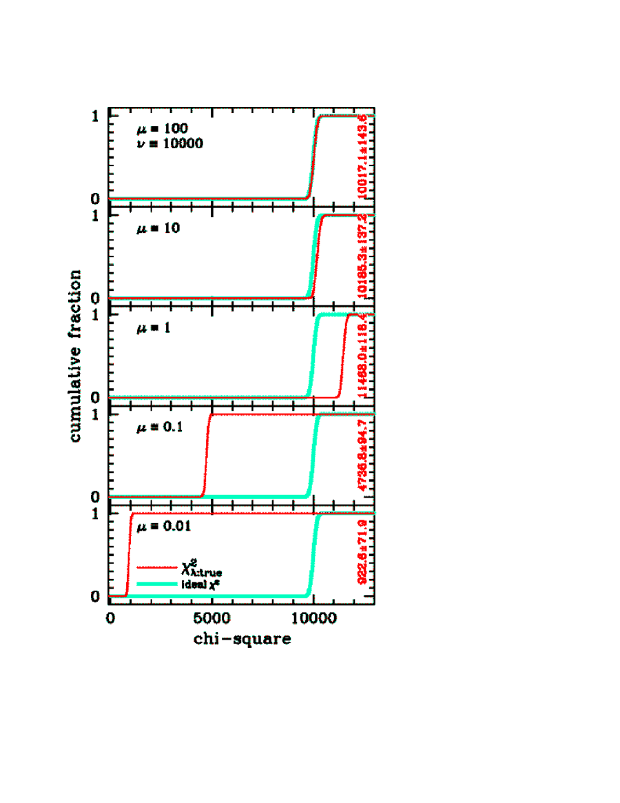
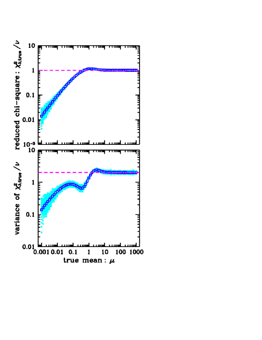
Let us continue the investigation of the performance of the Maximum Likelihood Ratio statistic for Poisson distributions with 1000 samples of $10^{4}$ Poisson deviates with Poisson mean values of 100, 10, 1, 0.1, and 0.001. Figure 2 confirms that the $\chi^{2}_{\lambda}$ statistic does not perform like an ideal $\chi^{2}$ statistic in the low-count regime. The average contribution by the $i$th deviate to an ideal $\chi^{2}$ statistic for the analysis of Poisson-distributed data would be exactly one and the average contribution to its variance would be exactly two. Figure 3 expands the previous analysis of PaperI of the $\chi^{2}_{\lambda}$ statistic over a wide range of Poisson mean values from 0.001 to 1000. The dashed lines of Fig. 3 show the results for an ideal $\chi^{2}$ statistic; one can clearly see that the average contribution to $\chi^{2}_{\lambda}$ is not equal to one and the average contribution to its variance is not equal to two for Poisson mean values $\mathrel{<\kern-10.00002pt\lower 3.87495pt\hbox{$\sim$}}$10. The poor performance of the $\chi^{2}_{\lambda}$ statistic with low-count data may come as a surprise to many readers since it has historically been advocated as being one of the best $\chi^{2}$ statistics for the analysis of Poisson-distributed data.

Chi-square statistics can serve (at least) two distinct purposes: (1) their functional forms can be utilized as the core of parameter estimation algorithms, and (2) their values can serve as a measure of the goodness-of-fit between a model and a data set.
$\bullet$ While the functional form of the $\chi^{2}_{\lambda}$ statistic can be successfully utilized for the purpose of parameter estimation with Poisson-distributed data in the low-count regime (see, e.g., PaperI), the Maximum Likelihood Ratio statistic for Poisson distributions [eq. (5)] should not be used to determine the goodness-of-fit with low-count data where the Poisson mean is $\mathrel{<\kern-10.00002pt\lower 3.87495pt\hbox{$\sim$}}$10.

In this work, I investigate the use of Pearson’s $\chi^{2}$ statistic and the chi-square-gamma statistic for the determination of the goodness-of-fit between theoretical models and data derived from counting experiments. I develop a methodology in §2 which modifies Pearsons’s chi-square statistic for the purpose of improving its goodness-of-fit performance. This methodology is then be applied to modify the chi-square-gamma statistic (§3). The modified chi-square-gamma statistic is shown to perform (nearly) like an ideal $\chi^{2}$ statistic for the determination of goodness-of-fit with low-count data. Simulated X-ray images are analyzed in §4 as a practical demonstration of the possible use of the modified chi-square-gamma statistic in experimental astrophysics. The summary of the paper is presented in §5.

2 THE MODIFIED PEARSON’S $\chi^{2}$ STATISTIC

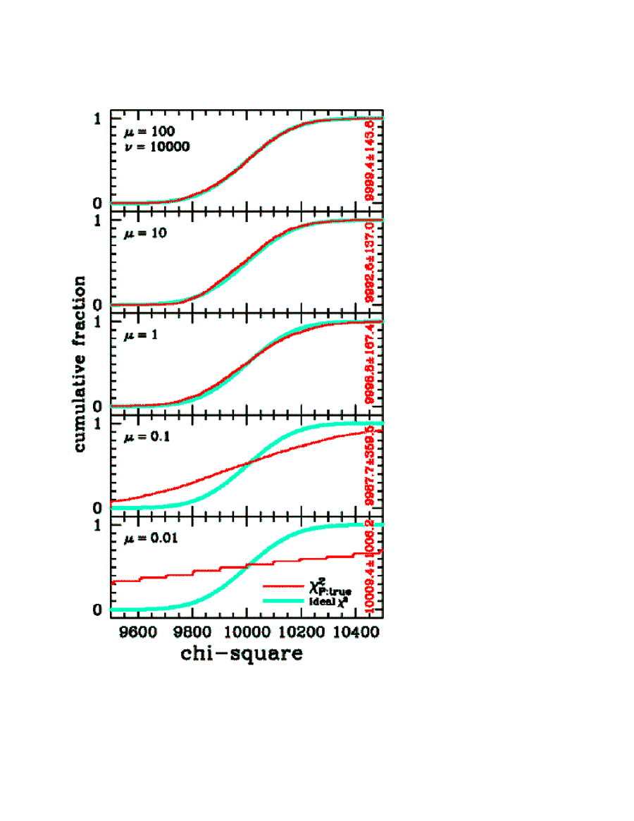
Let us continue the investigation of the performance of Pearson’s $\chi^{2}$ statistic with 1000 samples of $10^{4}$ Poisson deviates with Poisson mean values of 100, 10, 1, 0.1, and 0.001. Figure 4 shows that the $\chi^{2}_{\rm{P}}$ statistic does not perform like an ideal $\chi^{2}$ statistic for Poisson mean values $\mathrel{<\kern-10.00002pt\lower 3.87495pt\hbox{$\sim$}}\!10$. The average contribution by the $i$th deviate to an ideal $\chi^{2}$ statistic for the analysis of Poisson-distributed data would be exactly one and the average contribution to its variance would be exactly two. Figure 5 expands the previous analysis of PaperI of Pearson’s $\chi^{2}$ statistic over a wide range of Poisson mean values from 0.001 to 1000. The dashed lines of Fig. 5 show the results for an ideal $\chi^{2}$ statistic; one can see that while the average contribution to $\chi^{2}_{\rm{P}}$ is one, the average contribution to its variance is not equal to two for Poisson mean values $\mathrel{<\kern-10.00002pt\lower 3.87495pt\hbox{$\sim$}}\!10$.
$\bullet$ Pearson’s $\chi^{2}$ statistic [eq. (3)] should not be used to determine the goodness-of-fit with low-count data where the mean of the parent Poisson distribution is $\mathrel{<\kern-10.00002pt\lower 3.87495pt\hbox{$\sim$}}\!10$.

The variance of Pearson’s $\chi^{2}$ statistic is, by definition,

$$\sigma^{2}_{\chi^{2}_{\rm{P}}}\equiv{\sum_{i=1}^{N}}\left[\frac{(n_{i}-m_{i})^{2}}{m_{i}}-\left(\frac{1}{\nu}{\sum_{j=1}^{N}}\frac{(n_{j}-m_{j})^{2}}{m_{j}}\right)\right]^{2}\,,$$ (7)

where $\nu=N-M$ is the number of independent degrees of freedom, N is the number of data values, and M is the number of free parameters. The variance of the reduced chi-square of a $\chi^{2}$ statistic for a large number of observations should ideally be two. In the limit of a large number of observations of a single Poisson distribution with a mean value of $\mu$, the variance of the reduced chi-square of the Pearson’s $\chi^{2}$ statistic is

$$\sigma^{2}_{\chi^{2}_{\rm{P}}/\infty} \equiv \lim_{N\rightarrow\infty}\left[\frac{\sigma^{2}_{\chi^{2}_{\rm{P}}}}{\nu}\right]$$ (8)

$$\equiv \lim_{N\rightarrow\infty}\left[\frac{1}{\nu}~{}{\sum_{i=1}^{N}}\left\{\frac{(n_{i}-m_{i})^{2}}{m_{i}}-\left[\frac{1}{\nu}~{}{\sum_{j=1}^{N}}\frac{(n_{j}-m_{j})^{2}}{m_{j}}\right]\right\}^{2}\right]$$

$$\equiv \lim_{N\rightarrow\infty}\left[\frac{1}{\nu}~{}{\sum_{i=1}^{N}}\left\{\frac{(n_{i}-m_{i})^{2}}{m_{i}}-\left[\frac{\chi^{2}_{\rm{P}}}{\nu}\right]\right\}^{2}\right]$$

$$\approx \lim_{N\rightarrow\infty}\left[\frac{1}{\nu}~{}{\sum_{i=1}^{N}}\left\{\frac{(n_{i}-m_{i})^{2}}{m_{i}}-\lim_{N\rightarrow\infty}\left[\frac{\chi^{2}_{\rm{P}}}{\nu}\right]\right\}^{2}\right]$$

$$= \lim_{N\rightarrow\infty}\left[\frac{1}{N-M}~{}{\sum_{i=1}^{N}}\left\{\frac{(n_{i}-m_{i})^{2}}{m_{i}}-1\right\}^{2}\right]\hskip 62.59605pt\mbox{[see eq.\ (25) of \hbox{{\sc{PaperI}}}]}$$

$$= \lim_{N\rightarrow\infty}\left[\frac{1}{N-1}~{}{\sum_{i=1}^{N}}\left\{\frac{(n_{i}-\mu_{\rm{P}})^{2}}{\mu_{\rm{P}}}-1\right\}^{2}\right]\hskip 71.13188pt\mbox{[see eq.\ (5) of \hbox{{\sc{PaperI}}}]}$$

$$\approx \lim_{N\rightarrow\infty}\left[\frac{1}{N-1}~{}{\sum_{i=1}^{N}}\left\{\frac{\left(n_{i}-{\displaystyle\lim_{N\rightarrow\infty}}[\mu_{\rm{P}}]\right)^{2}}{{\displaystyle\lim_{N\rightarrow\infty}}[\mu_{\rm{P}}]}-1\right\}^{2}\right]$$

$$= \lim_{N\rightarrow\infty}\left[\frac{1}{N-1}~{}{\sum_{i=1}^{N}}\left\{\frac{(n_{i}-\mu)^{2}}{\mu}-1\right\}^{2}\right]\hskip 76.82243pt\mbox{[see eq.\ (7) of \hbox{{\sc{PaperI}}}]}$$

$$\approx \lim_{N\rightarrow\infty}\left[\frac{1}{N-1}~{}{\sum_{k=0}^{\infty}}\left\{NP(k;\mu)\right\}\left\{\frac{(k-\mu)^{2}}{\mu}-1\right\}^{2}\right]$$

$$= \frac{1}{\mu^{2}}~{}{\sum_{k=0}^{\infty}}P(k;\mu)\left[(k-\mu)^{2}-\mu\right]^{2}$$

$$= 2+\frac{1}{\mu}\ .$$

If we assume that Pearson’s $\chi^{2}$ applied to a large number of observations of a single Poisson distribution with a mean value of $\mu$ always produces a normal distribution with a mean equal to the number of degrees-of-freedom ($\nu$) [see eq. (25) of PaperI] and a variance of $\nu(2+\mu^{-1})$ [see eq. (8)], we can then attempt to create an ideal $\chi^{2}$ statistic for the analysis of Poisson-distributed data by modifying Pearson’s $\chi^{2}$ as follows:

$$\chi_{\rm{PM}}^{2}\equiv{\sum_{i=1}^{N}}\left[\left\{{\chi^{2}_{{\rm{P}}{i}}}-{\langle\chi^{2}_{{\rm{P}}i}\rangle}\right\}\left[{\frac{2}{\sigma^{2}_{\langle\chi^{2}_{{\rm{P}}i}\rangle}}}\right]^{1/2}\!\!+1\,\right]$$ (9)

where

$${\chi^{2}_{{\rm{P}}i}}\equiv\frac{(n_{i}-m_{i})^{2}}{m_{i}}$$ (10)

is the contribution of the $i$th data value to Pearson’s $\chi^{2}$,

$${\langle\chi^{2}_{{\rm{P}}i}\rangle}\equiv 1$$ (11)

is the expectation value of ${\chi^{2}_{{\rm{P}}i}}$ [see eq. (25) of PaperI],

$$\sigma^{2}_{\langle\chi^{2}_{{\rm{P}}i}\rangle}\equiv{2+m_{i}^{-1}}$$ (12)

is the variance of ${\langle\chi^{2}_{{\rm{P}}i}\rangle}$ [see eq. (8)]. Translating the mathematical notation to English, we have (1) shifted the mean of the standard $\chi^{2}_{\rm{P}}$ distribution from $\nu$ times equation (11) to zero, (2) forced the variance of the shifted distribution to be exactly $2\nu$, and then (3) shifted the mean of the variance-corrected distribution from zero back to $\nu$. Thus, by definition, the modified Pearson’s chi-square statistic ($\chi^{2}_{\rm{PM}}$) will have a mean value of $\nu$ and a variance of $2\nu$ — in the limit of a large number of observations.

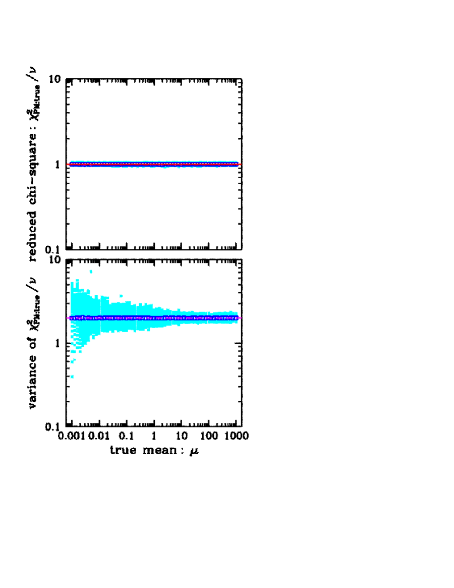
Let us now investigate the performance of the modified Pearson’s $\chi^{2}$ statistic with 1000 samples of $10^{4}$ Poisson deviates with Poisson mean values of 100, 10, 1, 0.1, and 0.001. Figure 6 shows that $\chi^{2}_{\rm{PM}}$ results are significantly better than $\chi^{2}_{\rm{P}}$ results [Fig. 4] — especially for Poisson mean values less than 10. Figure 7 investigates the performance of the modified Pearson’s $\chi^{2}$ statistic over a wide range of Poisson mean values from 0.001 to 1000. The dashed lines of Fig. 7 show the results for an ideal $\chi^{2}$ statistic; one can see that while the average contribution to $\chi^{2}_{\rm{PM}}$ is 1, as expected, and the average contribution to its variance is equal to 2, as expected, the performance is not uniform for all Poisson mean values — the spread seen in the variance plot (bottom panel) increases as the Poisson mean approaches zero.

Figures 6 and 7 indicate the the modified Pearson’s $\chi^{2}$ statistic works well in the perfect case where one has a priori knowledge of the true Poisson mean. In a real experiment, the true mean of the parent Poisson distribution is rarely (if ever) known and model parameters must be estimated from the observations. How well does the modified Pearson’s $\chi^{2}$ statistic work with reasonable parameter estimates? Comparing Fig. 8 with Fig. 6 and Fig. 9 with Fig. 7, we see that the variances are significantly smaller when a realistic model (i.e., the sample mean) is used instead of a perfect model (i.e., the true mean). A statistic that fails with reasonable parameter estimates is not a very useful statistic for the analysis of real observations with low-count data.
$\bullet$ The modified Pearson’s $\chi^{2}$ statistic [eq. (9)] should not be used to determine the goodness-of-fit with low-count data where the mean of the parent Poisson distribution is $\mathrel{<\kern-10.00002pt\lower 3.87495pt\hbox{$\sim$}}\!10$.

3 THE MODIFIED CHI-SQUARE-GAMMA STATISTIC

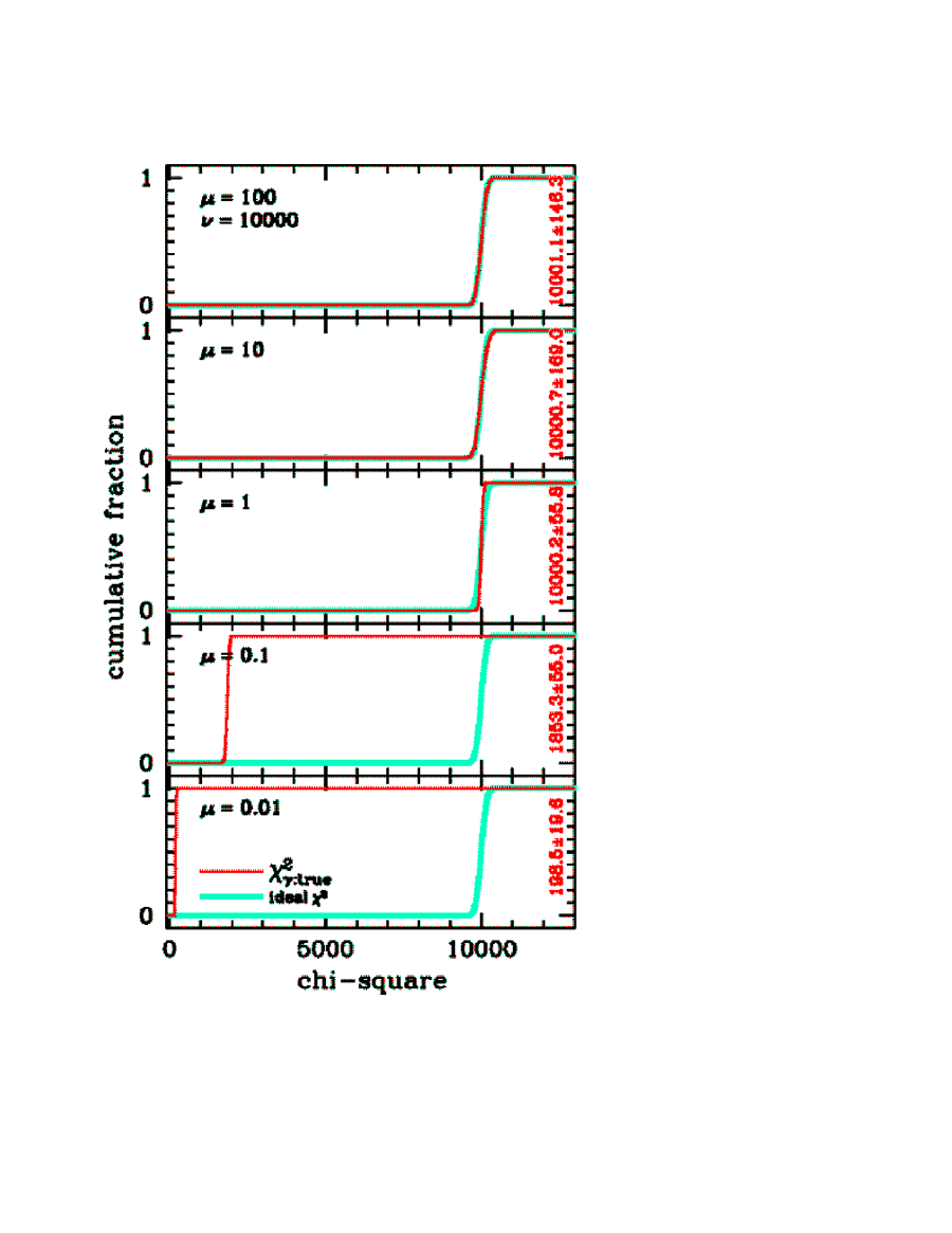
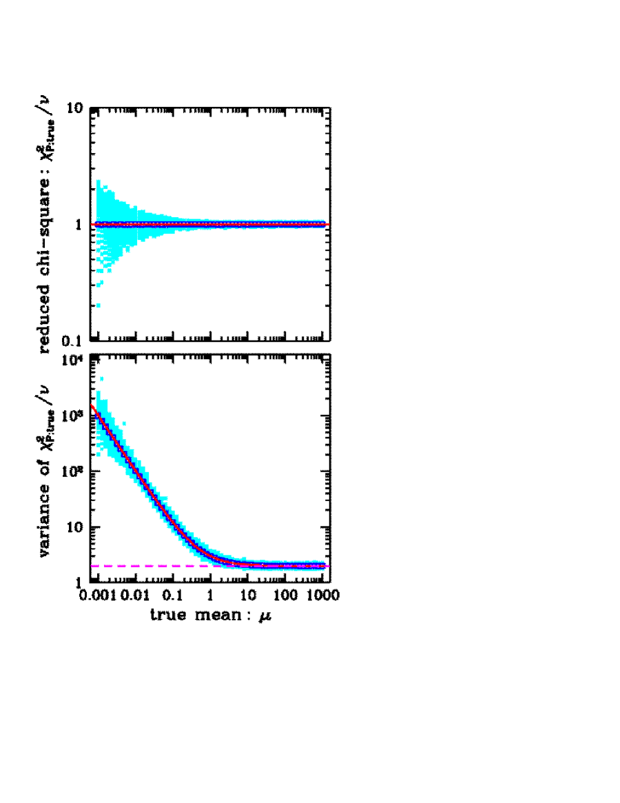
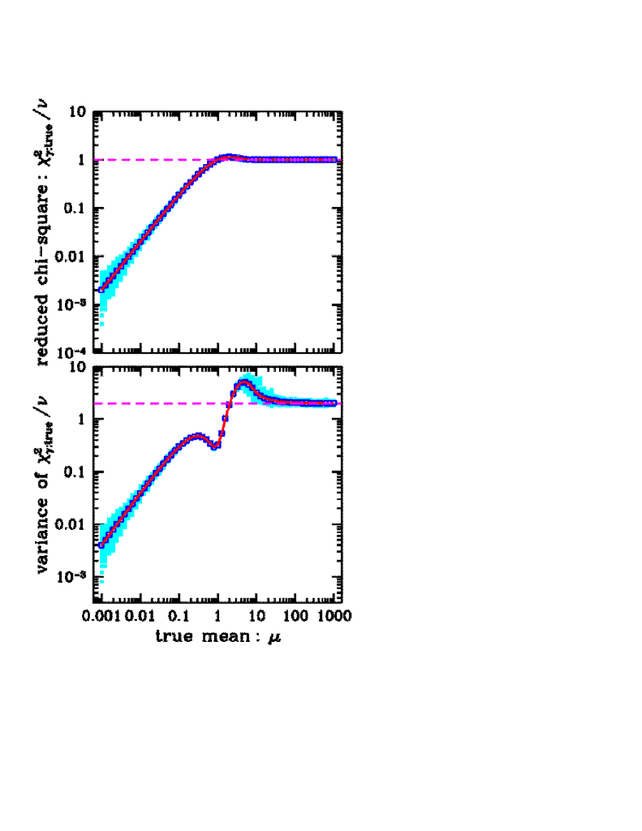
Let us continue the investigation of the performance of the chi-square-gamma statistic with 1000 samples of $10^{4}$ Poisson deviates with Poisson mean values of 100, 10, 1, 0.1, and 0.001. Figure 10 confirms that the $\chi^{2}_{\gamma}$ statistic does not perform like an ideal $\chi^{2}$ statistic in the low-count regime. Figure 11 expands the previous analysis of PaperI of the $\chi^{2}_{\gamma}$ statistic over a wide range of Poisson mean values from 0.001 to 1000. The $\chi^{2}_{\gamma}$ statistic clearly does not perform like an ideal $\chi^{2}$ statistic for Poisson mean values $\mathrel{<\kern-10.00002pt\lower 3.87495pt\hbox{$\sim$}}\!10$.
$\bullet$ The chi-square-gamma statistic [eq. (6)] should not be used to determine the goodness-of-fit with low-count data where the mean of the parent Poisson distribution is $\mathrel{<\kern-10.00002pt\lower 3.87495pt\hbox{$\sim$}}\!10$.

The variance of the chi-square-gamma statistic is, by definition,

$$\sigma^{2}_{\chi^{2}_{\gamma}}\equiv{\sum_{i=1}^{N}}\left[\frac{[n_{i}+{\rm{min}}(n_{i},1)-m_{i}]^{2}}{n_{i}+1}-\left(\frac{1}{\nu}{\sum_{j=1}^{N}}\frac{[n_{j}+{\rm{min}}(n_{j},1)-m_{j}]^{2}}{n_{j}+1}\right)\right]^{2}\,,$$ (13)

where $\nu=N-M$ is the number of independent degrees of freedom, N is the number of data values, and M is the number of free parameters. The variance of the reduced chi-square of a $\chi^{2}$ statistic for a large number of observations should ideally be two. In the limit of a large number of observations of a single Poisson distribution with a mean value of $\mu$, the variance of the reduced chi-square of the chi-square-gamma statistic is

$$\sigma^{2}_{\chi^{2}_{\gamma}/\infty} \equiv \lim_{N\rightarrow\infty}\left[\frac{\sigma^{2}_{\chi^{2}_{\gamma}}}{\nu}\right]$$ (14)

$$\equiv \lim_{N\rightarrow\infty}\left[\frac{1}{\nu}~{}{\sum_{i=1}^{N}}\left\{\frac{\left[n_{i}+{\rm{min}}(n_{i},1)-m_{i}\right]^{2}}{n_{i}+1}-\left[\frac{1}{\nu}~{}{\sum_{j=1}^{N}}\frac{\left[n_{j}+{\rm{min}}(n_{j},1)-m_{j}\right]^{2}}{n_{j}+1}\right]\right\}^{2}\right]$$

$$\equiv \lim_{N\rightarrow\infty}\left[\frac{1}{\nu}~{}{\sum_{i=1}^{N}}\left\{\frac{\left[n_{i}+{\rm{min}}(n_{i},1)-m_{i}\right]^{2}}{n_{i}+1}-\left[\frac{\chi^{2}_{\gamma}}{\nu}\right]\right\}^{2}\right]$$

$$\approx \lim_{N\rightarrow\infty}\left[\frac{1}{\nu}~{}{\sum_{i=1}^{N}}\left\{\frac{\left[n_{i}+{\rm{min}}(n_{i},1)-m_{i}\right]^{2}}{n_{i}+1}-\lim_{N\rightarrow\infty}\left[\frac{\chi^{2}_{\gamma}}{\nu}\right]\right\}^{2}\right]$$

$$= \lim_{N\rightarrow\infty}\left[\frac{1}{N-M}~{}{\sum_{i=1}^{N}}\left\{\frac{\left[n_{i}+{\rm{min}}(n_{i},1)-m_{i}\right]^{2}}{n_{i}+1}-\left[1+e^{-\mu}\left(\mu-1\right)\right]\right\}^{2}\right]\hskip 2.84526pt\mbox{[see eq.\ (29) of \hbox{{\sc{PaperI}}}]}$$

$$= \lim_{N\rightarrow\infty}\left[\frac{1}{N-1}~{}{\sum_{i=1}^{N}}\left\{\frac{\left[n_{i}+{\rm{min}}(n_{i},1)-\mu_{\gamma}\right]^{2}}{n_{i}+1}-\left[1+e^{-\mu}\left(\mu-1\right)\right]\right\}^{2}\right]\hskip 11.38109pt\mbox{[see eq.\ (18) of \hbox{{\sc{PaperI}}}]}$$

$$\approx \lim_{N\rightarrow\infty}\left[\frac{1}{N-1}~{}{\sum_{i=1}^{N}}\left\{\frac{\left[n_{i}+{\rm{min}}(n_{i},1)-{\displaystyle\lim_{N\rightarrow\infty}}[\mu_{\gamma}]\right]^{2}}{n_{i}+1}-\left[1+e^{-\mu}\left(\mu-1\right)\right]\right\}^{2}\right]$$

$$= \lim_{N\rightarrow\infty}\left[\frac{1}{N-1}~{}{\sum_{i=1}^{N}}\left\{\frac{\left[n_{i}+{\rm{min}}(n_{i},1)-\mu\right]^{2}}{n_{i}+1}-\left[1+e^{-\mu}\left(\mu-1\right)\right]\right\}^{2}\right]\hskip 17.07164pt\mbox{[see eq.\ (19) of \hbox{{\sc{PaperI}}}]}$$

$$\approx \lim_{N\rightarrow\infty}\left[\frac{1}{N-1}~{}{\sum_{k=0}^{\infty}}\left\{NP(k;\mu)\right\}\left\{\frac{\left[k+{\rm{min}}(k,1)-\mu\right]^{2}}{k+1}-\left[1+e^{-\mu}\left(\mu-1\right)\right]\right\}^{2}\right]$$

$$= {\sum_{k=0}^{\infty}}P(k;\mu)\left\{\frac{\left[k+{\rm{min}}(k,1)-\mu\right]^{2}}{k+1}-\left[1+e^{-\mu}\left(\mu-1\right)\right]\right\}^{2}$$

$$= \mu^{3}e^{-\mu}\left[{\rm{Ei}}(\mu)-\gamma_{\rm{EM}}-{\rm{ln}}(\mu)+4\right]-\mu^{2}-\mu+e^{-\mu}\!\left[-2\mu^{2}+2\mu+1\right]+e^{-2\mu}\!\left[-\mu^{2}+2\mu-1\right]\!,$$

where Ei$(x)$ is the exponential integral of $x$ $[\mbox{Ei}(x)=-\int_{-x}^{\infty}\frac{e^{-t}}{t}\,dt=\int_{-\infty}^{x}\frac{e^{-t}}{t}\,dt\mbox{~{}for~{}}x\!>\!0]$ and $\gamma_{\rm{EM}}\equiv\lim_{n\rightarrow\infty}\left[\left\{\sum_{i=1}^{n}\frac{1}{n}\right\}-\ln(n)\right]\approx 0.5772156649$ is the Euler-Mascheroni constant. Equation (14) approaches the expected value of 2 for large Poisson mean values [see the solid curve in the bottom panel of Fig. 11].

If we assume that chi-square-gamma statistic is applied to a large number of observations of a single Poisson distribution with a mean value of $\mu$ always produces a normal distribution with a mean equal to the number of degrees of freedom ($\nu$) times see equation (29) of PaperI and a variance of $\nu$ times equation (14), we can then attempt to create an ideal $\chi^{2}$ statistic for the analysis of Poisson-distributed data by modifying the chi-square-gamma statistic as follows:

$$\chi_{\rm{\gamma{M}}}^{2}\equiv{\sum_{i=1}^{N}}\left[\left\{{\chi^{2}_{{\gamma}i}}-{\langle\chi^{2}_{\gamma{i}}\rangle}\right\}\left[{\frac{2}{\sigma^{2}_{\langle\chi^{2}_{\gamma{i}}\rangle}}}\right]^{1/2}\!\!+1\,\right]$$ (15)

where

$${\chi^{2}_{{\gamma}i}}\equiv\frac{\left[n_{i}+\min\left(n_{i},1\right)-m_{i}\right]^{2}}{n_{i}+1}$$ (16)

is the contribution of the $i$th data value to the chi-square gamma statistic,

$${\langle\chi^{2}_{\gamma{i}}\rangle}\equiv 1+e^{-m_{i}}\left(m_{i}-1\right)$$ (17)

is the expectation value of ${\chi^{2}_{{\gamma}i}}$ [see equation (29) of PaperI], and

$$\sigma^{2}_{\langle\chi^{2}_{\gamma{i}}\rangle} \equiv m_{i}^{3}e^{-m_{i}}\left[{\rm{Ei}}(m_{i})-\gamma_{\rm{EM}}-{\rm{ln}}(m_{i})+4\right]-m_{i}^{2}-m_{i}+$$ (18)

$$e^{-m_{i}}\left[-2m_{i}^{2}+2m_{i}+1\right]+e^{-2m_{i}}\left[-m_{i}^{2}+2m_{i}-1\right]$$

is the variance of ${\langle\chi^{2}_{\gamma{i}}\rangle}$ [see equation (14)]. Translating the mathematical notation to English, we have (1) shifted the mean of the standard $\chi^{2}_{\rm{P}}$ distribution from $\nu$ times equation (17) to zero, (2) forced the variance of the shifted distribution to be exactly $2\nu$, and then (3) shifted the mean of the variance-corrected distribution from zero back to $\nu$. Thus, by definition, the modified chi-square statistic statistic ($\chi^{2}_{\gamma\rm{M}}$) will have a mean value of $\nu$ and a variance of $2\nu$ — in the limit of a large number of observations.

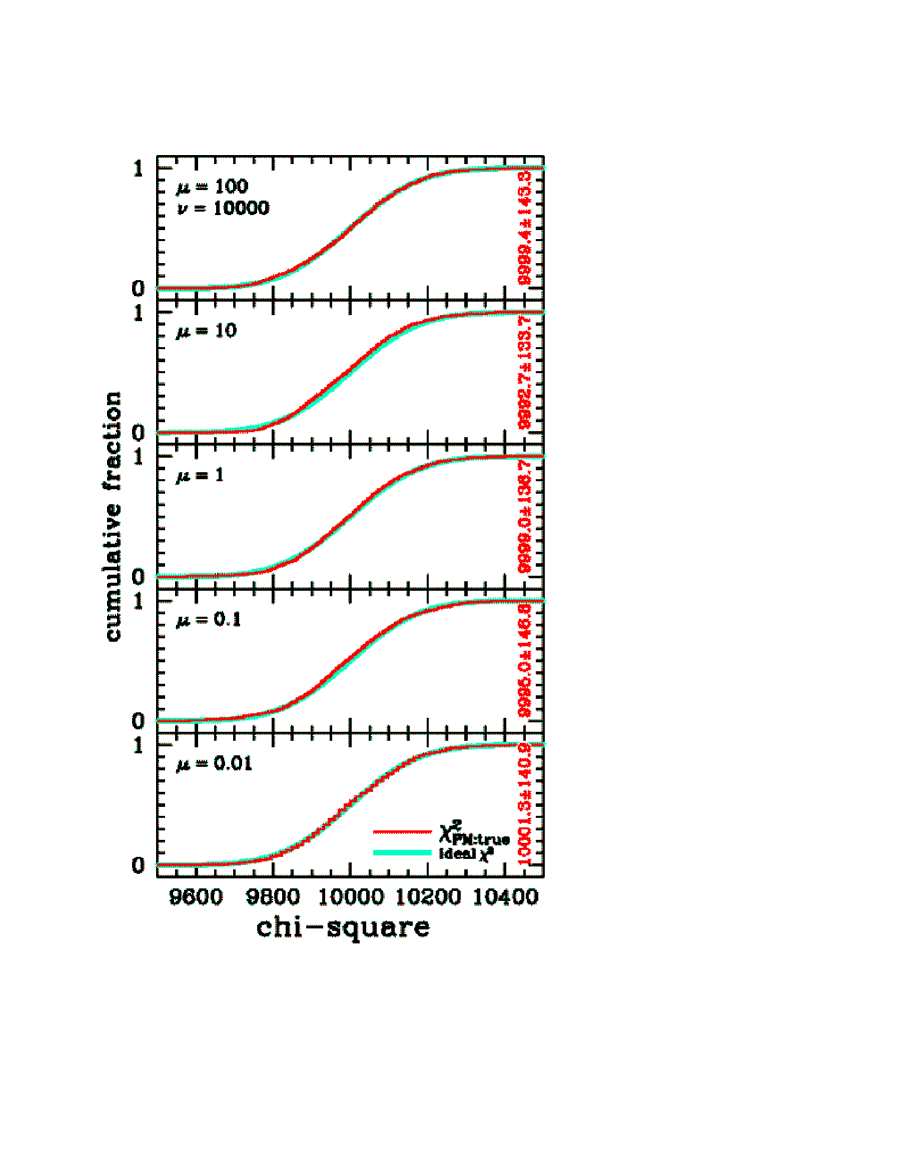
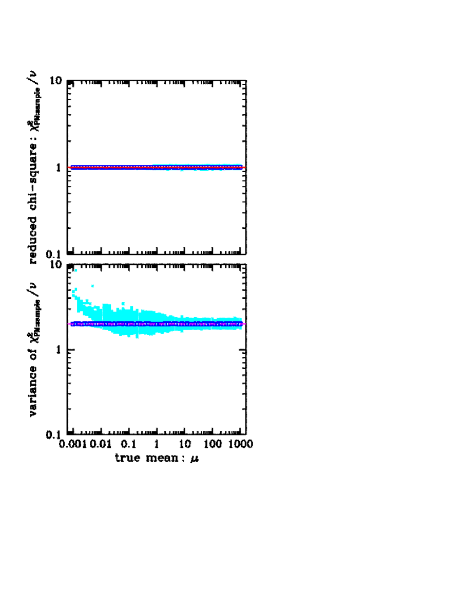
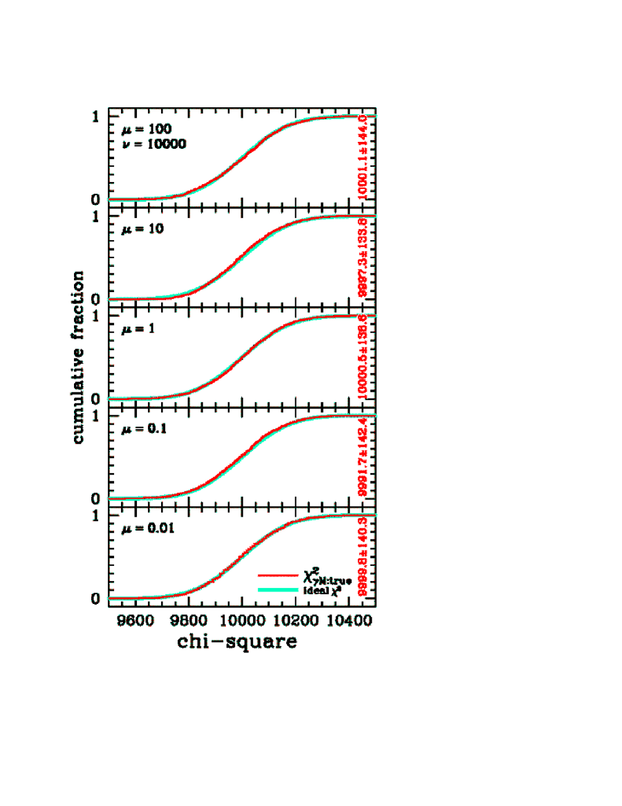
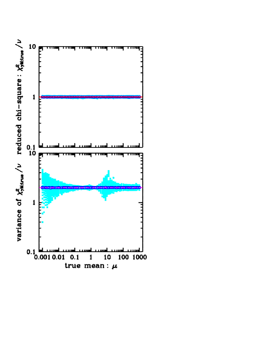
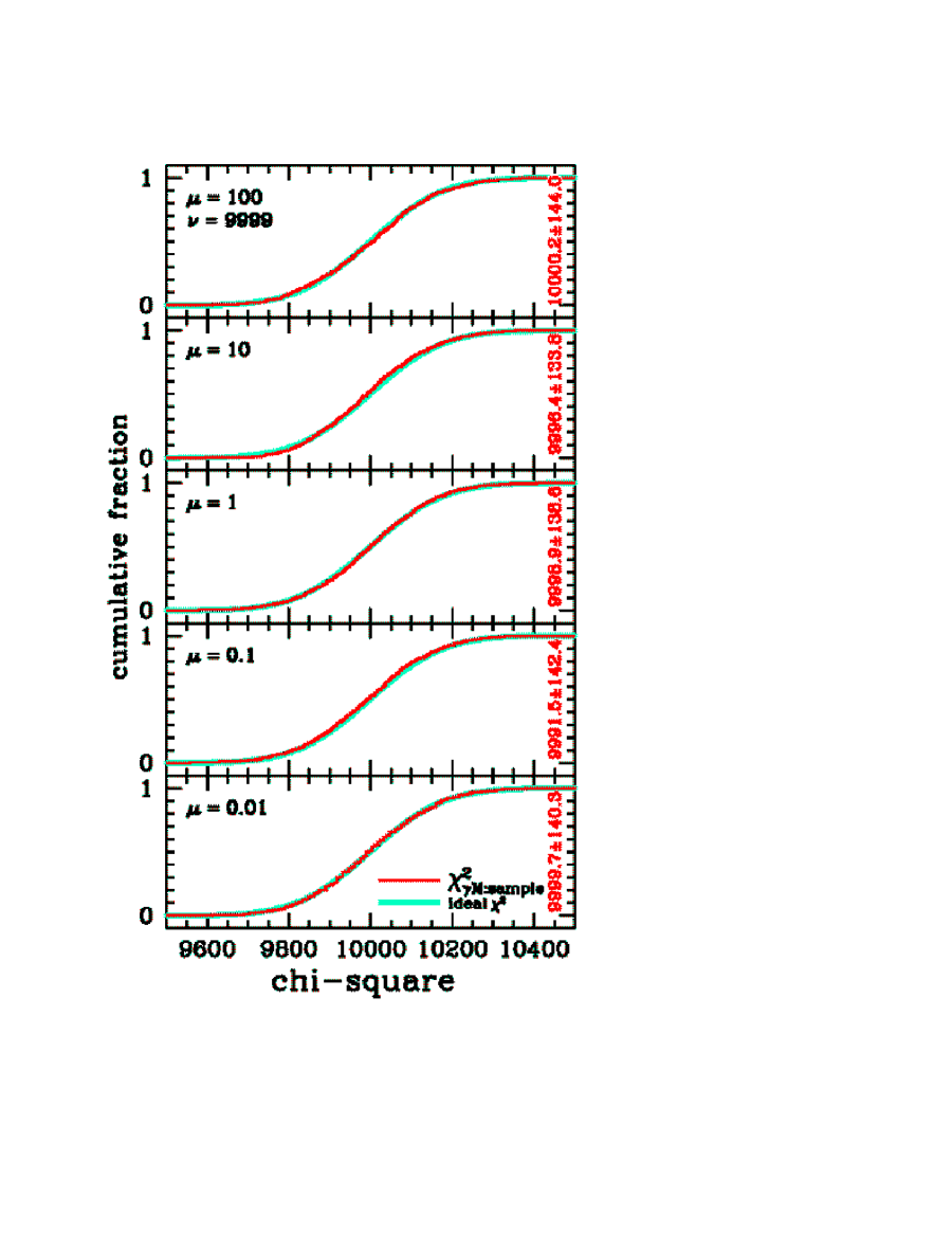
Let us now investigate the performance of the modified chi-square-gamma statistic with 1000 samples of $10^{4}$ Poisson deviates with Poisson mean values of 100, 10, 1, 0.1, and 0.001. Figure 12 shows that $\chi^{2}_{\gamma\rm{M}}$ results are significantly better than the $\chi^{2}_{\gamma}$ results [Fig. 10] — especially for Poisson mean values less than 10. Figure 13 investigates the performance of the $\chi^{2}_{\gamma\rm{M}}$ statistic over a wide range of Poisson mean values from 0.001 to 1000. The dashed lines of Fig. 13 show the results for an ideal $\chi^{2}$ statistic; one can see that while the average contribution to $\chi^{2}_{\gamma\rm{M}}$ is 1, as expected, and the average contribution to its variance is equal to 2, as expected, the performance is not uniform for all Poisson mean values. The bump seen in the bottom panel of Fig. 13 near the Poisson mean value of 10 is an artifact caused by the $\rm{min}(n_{i},1)$ offset in the numerator of the definition of the chi-square-gamma statistic [eq. (6)].

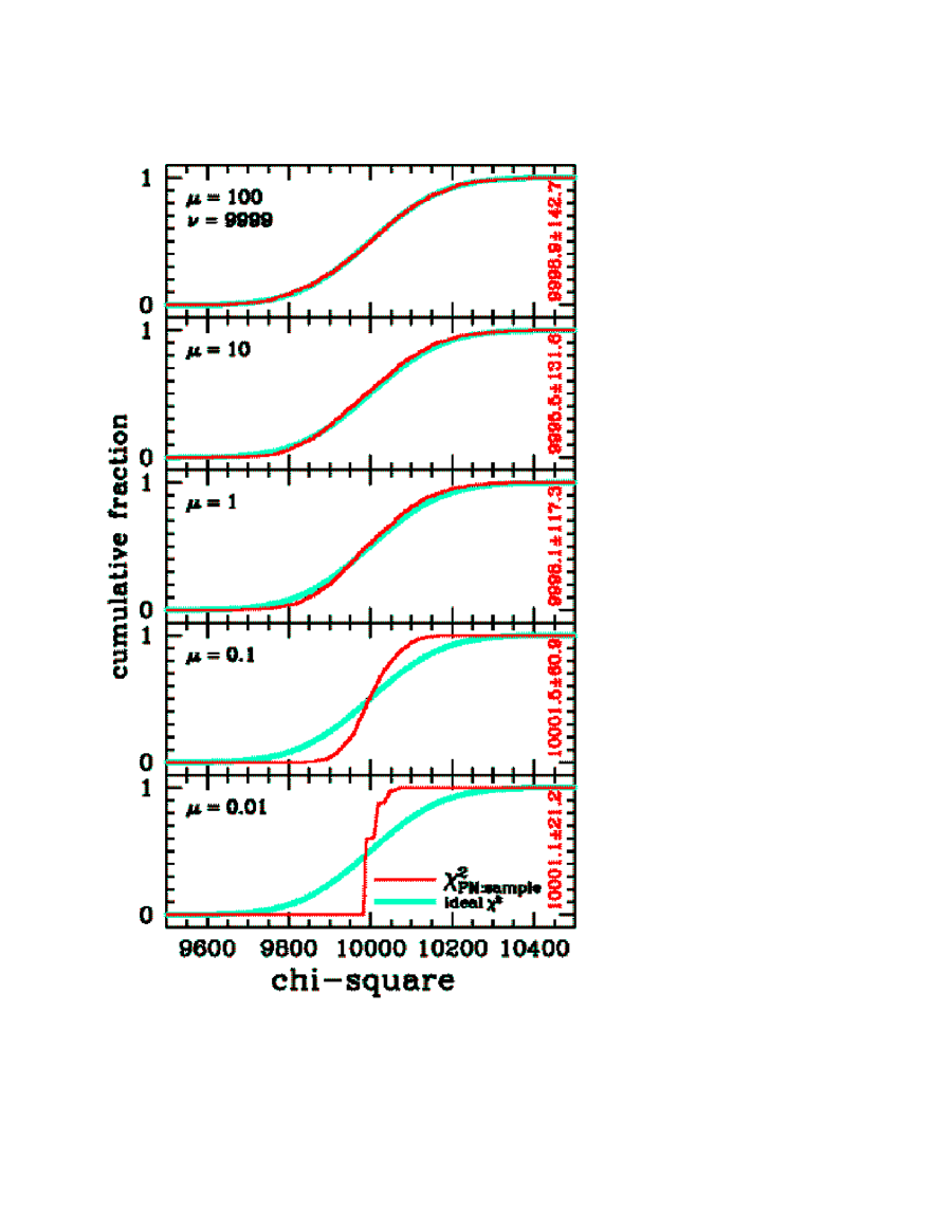
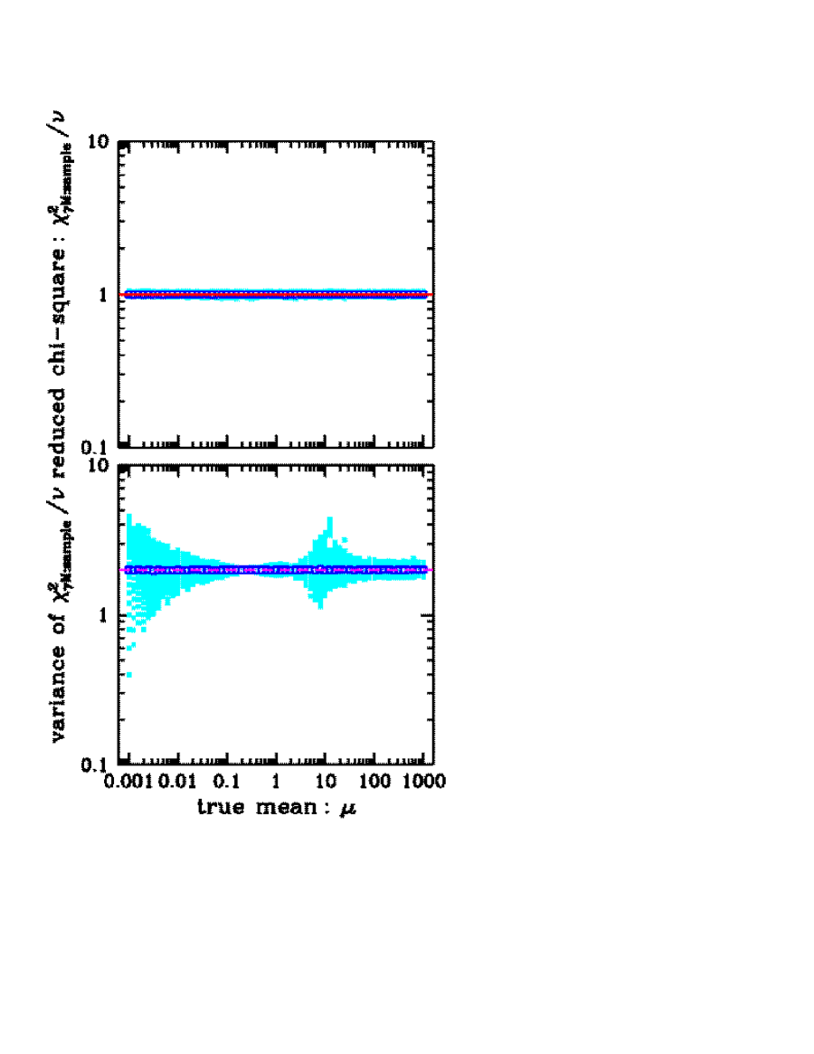
Figures 12 and 13 indicate the the modified chi-square-gamma statistic works well in the perfect case where one has a priori knowledge of the true Poisson mean. How well does the modified chi-square-gamma statistic work with reasonable parameter estimates? Comparing Fig. 14 with Fig. 12 and Fig. 15 with Fig. 13, we see that the results for the modified $\chi^{2}_{\gamma}$ statistic with a realistic model (i.e., the sample mean) are nearly identical to those obtained with a perfect model (i.e., the true mean).
$\bullet$ The modified chi-square-gamma [eq. (15)] statistic performs (nearly) like an ideal $\chi^{2}$ statistic for the determination of the goodness-of-fit with low-count data. On average, for a large number of observations, the mean value of $\chi^{2}_{\gamma\rm{M}}$ statistic is equal to the number of degrees of freedom $(\nu)$ and its variance is $2\nu$ — like the $\chi^{2}$ distribution for $\nu$ degrees of freedom.

4 SIMULATED X-RAY IMAGES

I now demonstrate the new modified chi-square-gamma statistic by using it to study simulated X-ray images. Cash (ca1979 (1979)) applied his $C$ statistic to the problem of determining the position of a weak source in a X-ray image. Let us use Cash’s Point Spread Function (PSF) but with a resolution of 100 pixels per unit area:

$$\phi(x,y)\equiv\left\{\begin{array}[]{ll}\displaystyle\frac{\pi}{3}\left(1-r\right)&\mbox{for $r\leq 1$,}\\ 0&\mbox{for $r>1$,}\end{array}\right.$$ (19)

where $r^{2}=(x/10)^{2}+(y/10)^{2}$. This PSF has the volume integral of

$$\Phi(x,y)\equiv\left\{\begin{array}[]{ll}\displaystyle 6\left[\frac{r^{2}}{2}-\frac{r^{3}}{3}\right]&\mbox{for $r\leq 1$,}\\ 1&\mbox{for $r>1$.}\end{array}\right.$$ (20)

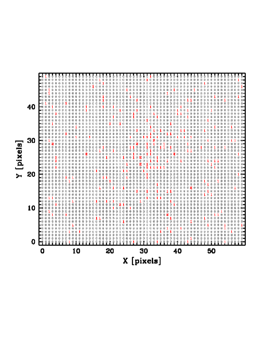
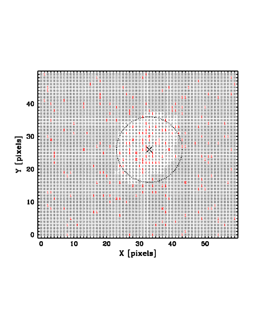
Figure 16 shows a simulated observation of a point source with an intensity of 40 X-ray photons on a background flux of 0.06 X-ray photons per pixel. This observation contains 2786 pixels with 0 photons, 204 pixels with 1 photons, and 10 pixels with 2 photons. There are a total of 56 photons found in the 317 pixels within a radius of 10 pixels of the center of the X-ray point source which is located at the $(x,y)$ position of $(33,26)$. This is clearly a marginal detection of a weak X-ray point source on a noisy background; the peak signal-to-noise ratio ($\sim$5.2) occurs at a radius of $\sim$8 pixels.

We will now use the modified chi-square-gamma statistic to answer the following questions about this X-ray image:

1. Is there an X-ray point source in the image?

2. If so, where is it located?

3. What is its total intensity?

The exact determination of the location and intensity of the X-ray point source in Fig. 16 is precluded by the fact that this particular observation contains only low-count data — we must be content with realistic estimates for the location and intensity based on a detailed statistical analysis of the data.

Our first objective is to determine if there is an X-ray point source in the observation. One way this can be done is to investigate the region(s) containing non-point-source pixels (data values). This approach requires knowledge of the background flux level — which we will henceforth assume is constant throughout the entire image. We begin by making a rough first estimate of the background flux level by dividing the total number of photon in the image by the total number of pixels: $0.0747$ $(\approx 224\,/\,3000)$ photons per pixel.

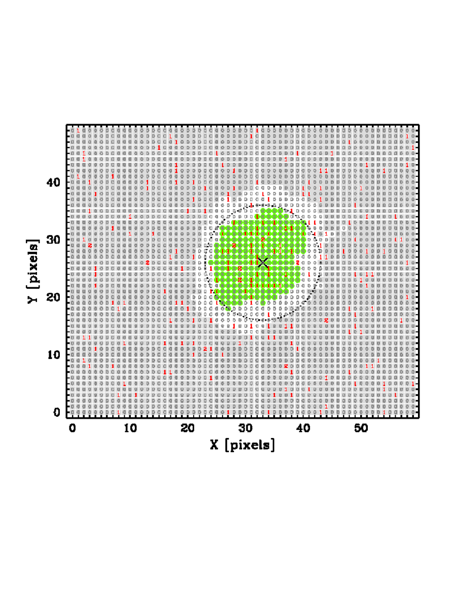
The background flux level estimate may be significantly improved with a bit more work. There are 18 photons in the 317 pixels within 10 pixels of the position $(12,15)$ of Fig. 16. Is the detection of 18 photons consistent with the expected value of 23.6799 $(=0.0747\times 317)$ photons? The upper and lower 99.9% single-sided confidence limits for 18 photons are 35.35 and 7.662, respectively [see Tables 1 and 2 of Gehrels ge1986 (1986)]. I conclude that the pixel at $(12,15)$ is a background pixel (shown as such with a gray box in Fig. 17) because the expected number of background photons lies within the range of the upper and lower 99.9% single-sided confidence limits of the observed number of photons (i.e., $7.662\leq 23.6799\leq 35.35$). There are 56 photons in the 317 pixels within 10 pixels of the position $(33,26)$ of Fig. 16. The upper and lower 99.9% single-sided confidence limits for 56 photons are 83.1784 and 35.6834, respectively [see eqs. (10) and (14) of Gehrels ge1986 (1986)]. I conclude that the pixel at $(33,26)$ is not a background pixel because the expected number of background photons is less than the lower 99.9% single-sided confidence limit of the observed number of photons (i.e., $23.6799<35.6834$). This conclusion was expected since $(33,26)$ is the center of the X-ray source. The 2676 gray pixels in Fig. 17 have a total of 162 photons. We can now make a second estimate of the background flux: $0.0605$ $(\approx 162\,/\,2676)$ photons per pixel. Repeating this process once more yields the final estimate of the background flux: $0.0601$ $(\approx 153\,/\,2547)$ photons per pixel. The measurement error for this estimate is approximately 0.0049 $(\approx\sqrt{153+1}\,/\,2547)$. The final estimate of the X-ray background flux, $0.0601\!\pm\!0.0049$, is in excellent agreement with the true value of 0.06 [see Fig. 18].

I conclude that Fig. 16 has at least one X-ray point source because the entire data set is not consistent with a X-ray background flux of 0.0601 photons per pixel for every pixel. Assuming that there is only one X-ray source, we can make the first rough estimate of its location by stating that it probably is located at a non-gray pixel location in Fig. 18. There are 453 non-background pixels in Fig. 18 with a total of 71 photons. This fact allows us to restrict the uncertainty of the location of the X-ray point source to about 15% $(\approx 453\,/\,3000)$ of the total image. Assuming a background flux of 0.06 photons per pixel, we expect that 27 $(\approx 453\times 0.06)$ photons of the total 71 photons found in the non-background pixels would be due to the background and not the point source. We can now make the first rough estimate of the intensity of the X-ray source: 44 $(=\!71\!-\!27)$ photons.

There are 48 photons in the 317 pixels within 10 pixels of the position $(24,26)$ of Fig. 16. Is this photon sum consistent with a model of a 40 photon point source centered at that location on a background of 0.06 photons per pixel? The upper and lower 95% single-sided confidence limits for 48 photons is 61.05 and 37.20 photons, respectively. The model predicts that we should find 58.9802 photons within a radius of 10 pixels. The 48 photons found within 10 pixels of $(24,26)$ is consistent with the model (shown as such with a dark-gray circle in Fig. 18), because the expected number of photons lies within the range of the upper and lower 95% single-sided confidence limits of the observed number of photons (i.e., $37.20\leq 58.9802\leq 61.05$). There are 217 circled pixels in Fig. 18. This fact allows us to further restrict the uncertainty of the location of the X-ray point source to $\sim$7.2% $(\approx 217\,/\,3000)$ of the total image.

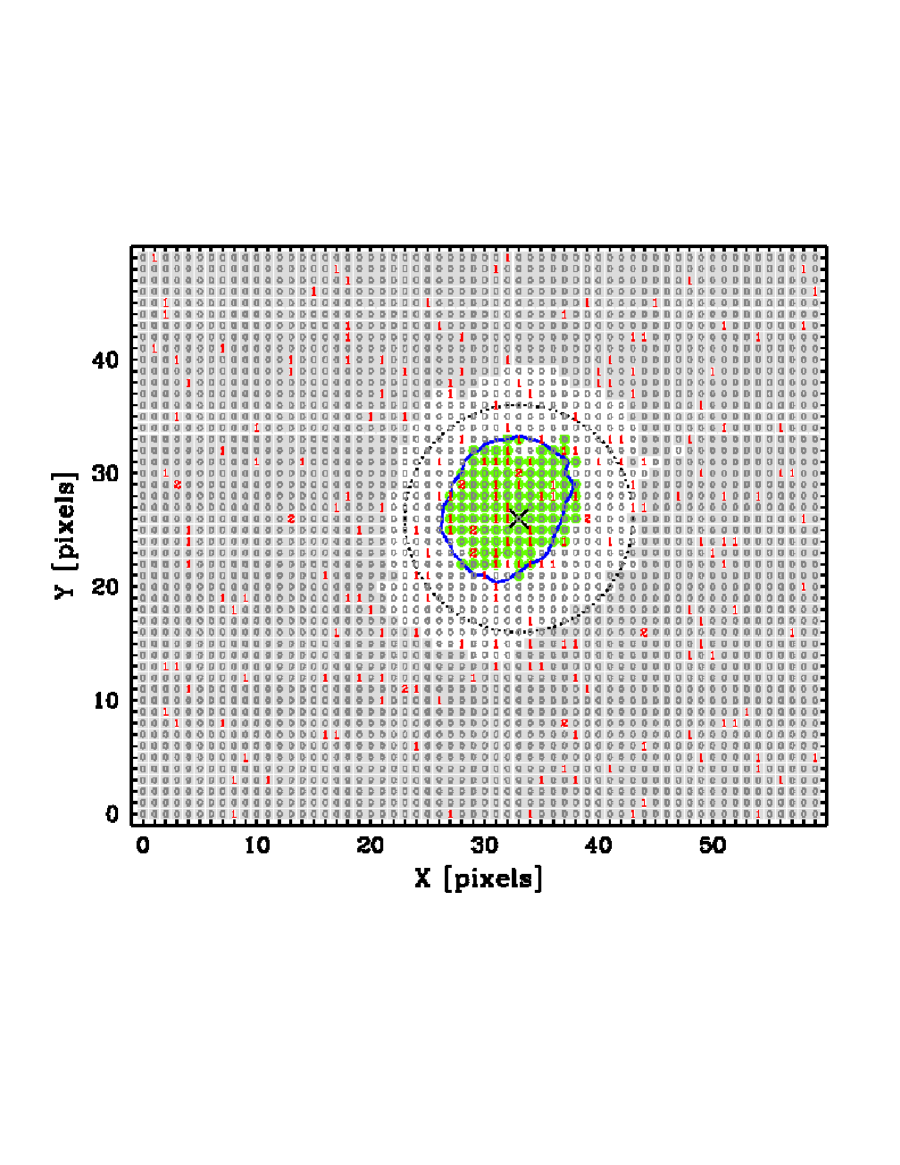
Since the peak signal-to-noise ratio occurs near a radius of 8 pixels, we now investigate if we can improve our estimate of the location of the X-ray point source by considering photon sums within a smaller aperture with a radius of 8 instead of 10 pixels. There are 34 photons in the 197 pixels within a radius of 8 pixels of the position $(26,26)$ of Fig. 16. Is this photon sum consistent with a model of a 40 photon point source centered at that location with a background of 0.06 photons per pixel? The upper and lower 95% single-sided confidence limits for 34 photons is 45.27 and 25.01 photons, respectively. The model predicts that we should find 47.2664 photons within a radius of 8 pixels. The 34 photons found within 8 pixels of $(26,26)$ is not consistent with the model since the expected number of photons is greater than the upper 95% single-sided confidence limit of the observed number of photons (i.e., $47.2664>45.27$). However, the 39 photons found within 8 pixels of $(27,26)$ is consistent with a 40 photon point source centered at $(27,26)$ on a background of 0.06 photons per pixel (i.e., $29.33\leq 47.2664\leq 50.94$). There are a total of 111 circled pixels in Fig. 19 . This fact allows us to further restrict the uncertainty of the location of the X-ray point source to $\sim$3.7% $(=111\,/\,3000)$ of the total image.

One way to boost the data out of the low-count regime is to compare the cumulative radial distribution of the model with the cumulative radial distribution of the data. The modified chi-square-gamma statistic was used to compare the cumulative radial distribution of the model (10 1-pixel-wide bins $\Rightarrow$ 10 degrees-of-freedom) with the cumulative radial distribution of the data (similarly formatted). At the position of $(27,26)$ the value of $\chi^{2}_{\gamma{\rm M}}$ for the cumulative radial distributions was computed to be 13.7338 ($\nu\equiv 10$) for a model of a 40 photon point source centered at $(27,26)$ on a background of 0.06 photons per pixel. The 95th percentage point for the chi-square distribution with 10 degrees of freedom may be found in several standard references: 18.3 (CRC Handbook of Chemistry and Physics, Lide & Frederikse crc1994 (1995), p. A-106), 18.31 (Bevington be1969 (1969), p. 315) and 18.3070 (Abramowitz & Stegun abst1964 (1964), p. 985). I conclude that the image location $(27,26)$ is within the 95% confidence interval because the value of the modified chi-square-gamma statistic is less than the 95th percentage point for the chi-square distribution with 10 degrees of freedom (i.e. $13.7338\!<\!18.3070$). The probability that the observed chi-square value for a correct model should be less than a value of $\chi^{2}$ for $\nu$ degrees of freedom is $P(\chi^{2}|\nu)=P(\frac{\nu}{2},\frac{\chi^{2}}{2})$ where the latter function is the incomplete gamma function [ $P\equiv 1-Q$; see, e.g., the GAMMP routine in Numerical Recipes (Press et al. pret1986 (1986))]. If we assume that $\chi^{2}_{\gamma{\rm M}}$ is distributed like the $\chi^{2}$ distribution, then we can assign a probability for the modified chi-square-gamma value for 10 degrees of freedom: $P(13.7338|10)=P(\frac{10}{2},\frac{13.7338}{2})=0.814517$. There is thus a $\sim$81.5% chance that the observed modified chi-square-gamma statistic will be less than 13.7338 for 10 degrees of freedom. The contour in Fig. 19 shows the 95% confidence interval of the X-ray point source based on the $\chi^{2}_{\gamma{\rm M}}$ analysis of the cumulative radial distribution of the data. The value of $\chi^{2}_{\gamma{\rm M}}$ for the cumulative radial distribution at $(26,26)$ was computed to be 30.4707 giving a probability of $\sim$99.9%; this location in Fig. 19 lies outside the 95% confidence interval.

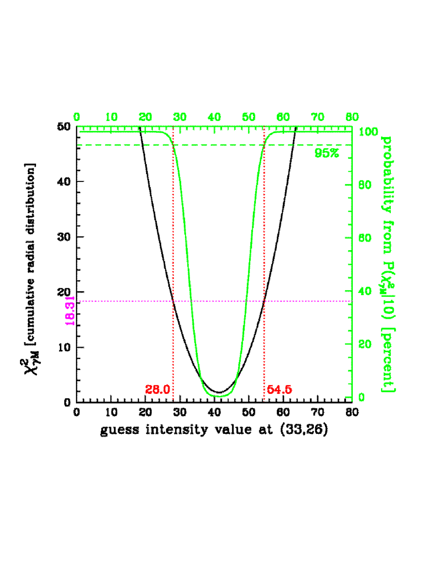
We can further use the modified chi-square-gamma statistic with the cumulative radial distribution to determine the 95% confidence limits of the intensity of the X-ray source in the image (see Fig. 20 ). The upper and lower single-sided 95% confidence limits for the intensity of an X-ray point source at $(33,26)$ in Fig. 16 is 54.5 and 28.0, respectively. The true intensity of the X-ray source is 40 photons. Given a background flux uncertainty of $\sigma_{B}=0.0049$ photons per pixel (see above), we can approximate the theoretical rms measurement error for a 40 photon point source spread over 317 pixels $(A=317$ px${}^{2})$ as $\sigma\approx\sqrt{40+1}+A\sigma_{B}\approx 8.0$ photons. The difference between the upper and lower 95% single-sided confidence limits is approximately 3.3 standard deviations of the normal probability function. This fact can be used to approximate an rms measurement error for our intensity estimate of $\sigma_{I}\approx 8.0$ [$\approx(54.5-28.0)/(2\times 1.65)$] photons. The $\chi^{2}_{\gamma{\rm M}}$ analysis using the cumulative radial distribution has yielded an excellent intensity estimate.

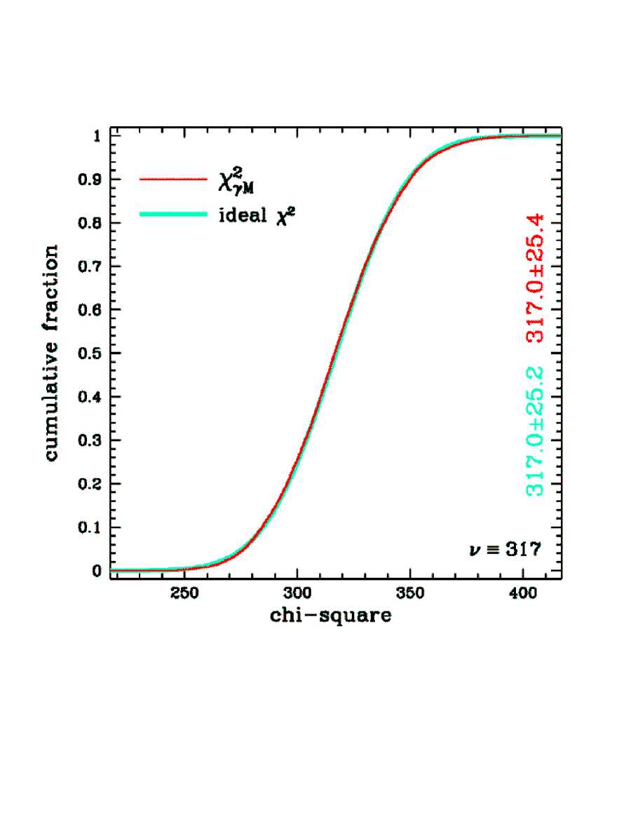
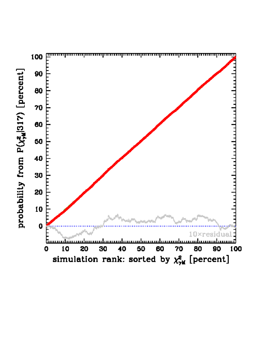
The analysis presented in Figures 19 and 20 is predicated on the assumption that the modified chi-square-gamma statistic is distributed like $\chi^{2}$. But is this assumption valid? Figure 21 shows that the analysis of $10^{4}$ simulated X-ray observations like Fig. 16 yields modified chi-square-gamma values that are distributed like the chi-square distribution for $\nu\equiv 317$ degrees of freedom: a Gaussian distribution with a mean of $\nu$ and a variance of $2\nu$. The above analysis has assumed that the probability that the observed modified chi-square-gamma value for a correct model should be less than a value of $\chi^{2}$ for $\nu$ degrees of freedom can be given as $P(\chi^{2}_{\gamma{\rm M}}|\nu)$. Assuming that the predicted probability from $P(\chi^{2}_{\gamma{\rm M}}|\nu)$ is an accurate prediction of the true probability, then the predicted probability of the 9500th simulated observation of a total of 10000 (sorted by $\chi^{2}_{\gamma{\rm M}}$ value) should be very close to 95%; Fig. 22 indicates that this is indeed the case (i.e., the probability for the $\chi^{2}_{\gamma{\rm M}}$ value of the 9500th simulated observation is 94.8666%). Since $\chi^{2}_{\gamma{\rm M}}$ statistic is distributed (nearly) like the $\chi^{2}$ distribution, the usage of the incomplete gamma function to predict probabilities for modified chi-square-gamma values appears to be justified in practical analysis problems.

5 SUMMARY

I investigated the use of Pearson’s chi-square statistic [eq. (3)], the Maximum Likelihood Ratio statistic for Poisson distributions [eq. (5)], and the chi-square-gamma statistic [eq. (6)] for the determination of the goodness-of-fit between theoretical models and low-count Poisson-distributed data. I concluded that none of these statistics should be used to determine the goodness-of-fit with data values of 10 or less.

I modified Pearson’s chi-square statistic for the purpose of improving its goodness-of-fit performance. I demonstrated that modified Pearson’s $\chi^{2}$ statistic [eq. (9)] works well in the perfect case where one has a priori knowledge of the correct (true) model. In a real experiment, however, the true mean of the parent Poisson distribution is rarely (if ever) known and model parameters must be estimated from the observations. I demonstrated that the modified Pearson’s $\chi^{2}$ statistic has a variance that is significantly smaller than that of the $\chi^{2}$ distribution when realistic models, defined as having parameters estimated from the observational data, are compared with Poisson-distributed data. Any statistic that fails with models based on reasonable parameter estimates is not a very practical statistic for the analysis of astrophysical observations. I concluded that the modified Pearson’s $\chi^{2}$ statistic should not be used to determine the goodness-of-fit with low-count data values of 10 or less.

I modified the chi-square-gamma statistic for the purpose of improving its goodness-of-fit performance. I demonstrated that the modified chi-square-gamma statistic [eq. (15)] performs (nearly) like an ideal $\chi^{2}$ statistic for the determination of goodness-of-fit with low-count data. On average, for correct (true) models, the mean value of the modified chi-square-gamma statistic is equal to the number of degrees of freedom $(\nu)$ and its variance is $2\nu$ — like the $\chi^{2}$ distribution for $\nu$ degrees of freedom.

An ideal $\chi^{2}$ statistic for the determination of goodness-of-fit with low-count data should fail in a predictable manner. Hypothesis testing of low-count Poisson-distributed data with the modified Pearson’s $\chi^{2}$ statistic will produce the peculiar and undesirable result that correct models are more likely to be rejected than realistic models [cf. Fig. 6 with Fig. 8]. The modified chi-square-gamma statistic is a practical statistic to use for hypothesis testing of astrophysical data from counting experiments because it performs (nearly) like an ideal $\chi^{2}$ statistic for realistic and correct models in the low-count and the high-count data regimes; accurate and believable probabilities for $\chi^{2}_{\gamma{\rm M}}$ goodness-of-fit values can be calculated with the incomplete gamma function [Figs. 21 and 22]. A lot of nothing can tell you something — as long as there are some observations with signal in them.

 

Figure 1: A simulated data set of 1000 samples (“observations”) of $10^{4}$ Poisson deviates (“measurements”) per sample was created assuming a mean value $\mu$$\equiv$$100$ for each Poisson deviate. Each sample in this data set was then analyzed using Pearson’s $\chi^{2}$ statistic [top; definition: eq. (3)], the Maximum Likelihood Ratio statistic for Poisson distributions [middle; definition: eq. (5)], and the chi-square-gamma statistic [bottom; definition: eq. (6)]. The model of the $i$th deviate in each sample was set to the true mean value of parent Poisson distribution (i.e., $m_{i}\!=\!\mu\!\equiv\!100$) and the number of independent degrees-of-freedom was therefore equal to the number of deviates per sample (i.e. $\nu\!\equiv\!10^{4}$). Compare the cumulative distribution for each statistic with the cumulative distribution function of a Gaussian distribution with a mean of $10^{4}$ and a variance of $2\!\times\!10^{4}$ [thick curve in each panel]. The number and error shown on the right side of each panel is the mean and rms value of the 1000 samples shown in that panel; ideally these values should be about $10000\!\pm\!141.4\,$.

Figure 2: The cumulative distribution functions for 1000 samples of $10^{4}$ Poisson deviates (top to bottom: $\mu\equiv 100,10,1,0.1$, and 0.01) analyzed using the Maximum Likelihood Ratio statistic for Poisson distributions [definition: eq. (5)]. In all cases, $\nu\!\equiv\!10^{4}$ and $m_{i}$ was set to the true mean value of the data set. Other details as in Fig. 1.

Figure 3: Top panel: Reduced chi-square as a function of the true Poisson mean ($0.001\leq\mu\leq 1000$ with 10 mean values per decade) for the Maximum Likelihood Ratio statistic for Poisson distributions with the model of the $i$th deviate set to the mean value of the parent Poisson distribution. The open squares show the results of the analysis of one sample composed of $10^{7}$ Poisson deviates ($\nu\equiv 10^{7}$) at each given Poisson mean value. The filled squares show the results of the analysis of 1000 subsamples of the $10^{7}$ Poisson deviates ($\nu\equiv 10^{4}$) previously analyzed as one large sample. The scatter of the filled squares with respect to the open squares is real and is due to random fluctuations of the parent Poisson distributions. The dashed line shows the ideal value of one. Bottom panel: The variance of the reduced chi-square values shown in the top panel. The dashed line shows the ideal value of two.

Figure 4: The cumulative distribution functions for 1000 samples of $10^{4}$ Poisson deviates (top to bottom: $\mu\equiv 100,10,1,0.1$, and 0.01) analyzed using Pearson’s $\chi^{2}$ statistic [definition: eq. (3)] (same input data set as for Fig. 2). In all cases, $\nu\!\equiv\!10^{4}$ and $m_{i}$ was set to the true mean value of the data set. Other details as in Fig. 1.

Figure 5: Reduced chi-square as a function of the true Poisson mean for Pearson’s $\chi^{2}$ statistic with the model of the $i$th deviate set to the true mean value of the parent Poisson distribution (same input data set as for Fig. 3). The solid line connecting the open squares in the bottom panel is the formula $2+\mu^{-1}$ [see eq. (8)]. Other details as in Fig. 3.

Figure 6: The cumulative distribution functions for 1000 samples of $10^{4}$ Poisson deviates (top to bottom: $\mu\equiv 100,10,1,0.1$, and 0.01) analyzed using the modified Pearson’s $\chi^{2}$ statistic [definition: eq. (9)] (same input data set as for Fig. 2). In all cases, $\nu\!\equiv\!10^{4}$ and $m_{i}$ was set to the true mean value of the data set. Other details as in Fig. 1.

Figure 7: Reduced chi-square as a function of the true Poisson mean for the modified Pearson’s $\chi^{2}$ statistic with the model of the $i$th deviate set to the true mean value of the parent Poisson distribution (same input data set as for Fig. 3). Other details as in Fig. 3.

Figure 8: The cumulative distribution functions for 1000 samples of $10^{4}$ Poisson deviates (top to bottom: $\mu\equiv 100,10,1,0.1$, and 0.01) analyzed using the modified Pearson’s $\chi^{2}$ statistic (same input data set as for Fig. 2). In all cases, $\nu\!\equiv\!10^{4}$ and $m_{i}$ was set to the sample mean. Other details as in Fig. 1.

Figure 9: Reduced chi-square as a function of the true Poisson mean for the modified Pearson’s $\chi^{2}$ statistic with the model of the $i$th deviate set to the sample mean (same input data set as for Fig. 3). Other details as in Fig. 3.

Figure 10: The cumulative distribution functions for 1000 samples of $10^{4}$ Poisson deviates (top to bottom: $\mu\equiv 100,10,1,0.1$, and 0.01) analyzed using the $\chi^{2}_{\gamma}$ statistic [definition: eq. (6)] (same input data set as for Fig. 2). In all cases, $\nu\!\equiv\!10^{4}$ and $m_{i}$ was set to the true mean value of the data set. Other details as in Fig. 1.

Figure 11: Reduced chi-square as a function of the true Poisson mean for the $\chi^{2}_{\gamma}$ statistic statistic with the model of the $i$th deviate set to the true mean value of the parent Poisson distribution (same input data set as for Fig. 3). The solid line connecting the open squares in the top panel is the formula $1+e^{-\mu}\left(\mu-1\right)$ [eq. 29 of PaperI]. The solid line connecting the open squares in the bottom panel is equation (14). Other details as in Fig. 3.

Figure 12: The cumulative distribution functions for 1000 samples of $10^{4}$ Poisson deviates (top to bottom: $\mu\equiv 100,10,1,0.1$, and 0.01) analyzed using the modified $\chi^{2}_{\gamma}$ statistic [definition: eq. (15)] (same input data set as for Fig. 2). In all cases, $\nu\!\equiv\!10^{4}$ and $m_{i}$ was set to the true mean value of the data set. Other details as in Fig. 1.

Figure 13: Reduced chi-square as a function of the true Poisson mean for the modified $\chi^{2}_{\gamma}$ statistic with the model of the $i$th deviate set to the true mean value of the parent Poisson distribution (same input data set as for Fig. 3). Other details as in Fig. 3.

Figure 14: The cumulative distribution functions for 1000 samples of $10^{4}$ Poisson deviates (top to bottom: $\mu\equiv 100,10,1,0.1$, and 0.01) analyzed using the modified $\chi^{2}_{\gamma}$ statistic (same input data set as for Fig. 2). In all cases, $\nu\!\equiv\!10^{4}$ and $m_{i}$ was set to the sample mean. Other details as in Fig. 1.

Figure 15: Reduced chi-square as a function of the true Poisson mean for the modified $\chi^{2}_{\gamma}$ statistic with the model of the $i$th deviate set to the sample mean (same input data set as for Fig. 3). Other details as in Fig. 3.

Figure 16: The simulated X-ray observation. A 40 photon X-ray point source is located at the $(x,y)$ position of $(33,26)$ on a background of 0.06 photons per pixel. The Point Spread Function is $\phi(x,y)\equiv(\pi/3)[1-\mbox{min}(r,1)]$ where $r^{2}=(x/10)^{2}+(y/10)^{2}$. This is the same PSF used by Cash (ca1979 (1979)) but with a resolution of 100 pixels per unit area.

Figure 17: Gray boxes indicate pixels with a total number of photons within a radius of 10 pixels that are consistent (within the 99.9% upper and lower single-sided confidence limits of the observed photon total) with the estimated background flux level of 0.0747 photons per pixel. The X marks the center of the X-ray point source and the dotted circle has a radius of 10 pixels which is the maximum size of the PSF. Other details as in Fig. 16.

Figure 18: Gray boxes indicate the pixels with a total number of photons within a radius of 10 pixels that are consistent (within the 99.9% upper and lower single-sided confidence limits of the observed photon total) with the true background flux level of 0.06 photons per pixel. Dark-gray circles indicate the pixels with a total number of photons within a radius of 10 pixels that are consistent (within the 95% upper and lower single-sided confidence limits of the observed photon total) with the model of a 40 photon point source at that pixel location on a background of 0.06 photons per pixel. Other details as in Fig. 17.

Figure 19: Dark-gray circles indicate the pixels with a total number of photons within a radius of 8 pixels that are consistent (within the 95% upper and lower single-sided confidence limits of the observed photon total) with the model of a 40 photon point source at that pixel location on a background of 0.06 photons per pixel. All pixels within the solid black contour are within the 95% confidence interval as determined by the $\chi^{2}_{\gamma{\rm M}}$ analysis of the cumulative radial distribution of the data within 10 pixels is compared with the cumulative radial distribution of a model of a 40 photon point source at that pixel location on a background of 0.06 photons per pixel. Note how well the 95% confidence interval of the $\chi^{2}_{\gamma{\rm M}}$ analysis of the cumulative radial distribution matches the region described by the circled pixels. Other details as in Fig. 18.

Figure 20: The photon distribution of the 317 pixels within a radius of 10 pixels of the location $(33,26)$ of Fig. 16 was transformed to a cumulative radial distribution (10 1-pixel-wide bins $\Rightarrow$ 10 degrees-of-freedom) and then compared, using the modified chi-square-gamma statistic, with 80 models of the observation: a 1 to 80 photon (in steps of 1 photon) X-ray point source at $(33,26)$ on a background of 0.06 photons per pixel (i.e., the true background). The 95th percentage point for the chi-square distribution with 10 degrees of freedom is 18.31 [i.e. $P(18.31|10)=0.95\,$]. Assuming that $\chi^{2}_{\gamma{\rm M}}$ is distributed like $\chi^{2}$, we see that the upper and lower single-sided 95% confidence limits for the intensity of an X-ray point source at $(33,26)$ in Fig. 16 is 54.5 and 28.0, respectively. The true intensity of the X-ray source is 40 photons.

Figure 21: A data set of $10^{4}$ realizations of the the same model used to make Fig. 16 was created. Each sample in this data set was then analyzed using the modified chi-square-gamma statistic at the location $(33,26)$ – the true location of the simulated X-ray point source of 40 photons on a background of 0.06 photons per pixel. All 317 pixels within a radius of 10 pixels (the size of the PSF) were compared to the true model value at that location and the number of independent degrees-of-freedom was therefore equal to the number of pixels analyzed (i.e. $\nu\!\equiv\!317$). Compare the cumulative distribution with the cumulative distribution function of a Gaussian distribution with a mean of $317$ and a variance of $\sqrt{2\!\times\!317}~{}(\approx 25.2)$ [thick curve]. The numbers with errors shown on the right side give the mean and rms value for the $\chi^{2}_{\gamma{\rm M}}$ (top) and ideal $\chi^{2}$ (bottom) statistics.

Figure 22: The $10^{4}$ simulations of Fig. 21 were sorted by the value of the modified chi-square-gamma statistic. The dark plot shows the probablity $P(\chi^{2}_{\gamma{\rm M}}|317)$ as a function of the sorted $\chi^{2}_{\gamma{\rm M}}$ values. The gray plot on the bottom shows the residuals from the ideal one-to-one correspondance. The predicted probabilities for the 9000th, 9500th, and 9900th sorted simulations were 90.2069%, 94.8666%, and 98.9497%, which agrees very well with the expected probabilities of 90%, 95%, and 99%, respectively. For the entire simulation, the mean and rms value of the resiuals is $0.0013\!\pm\!0.0038$ percentage points — note that the residuals never exceeds 1 percent. Figures 21 and 22 indicate that the assumption that the $\chi^{2}_{\gamma{\rm M}}$ statistic is distributed like the $\chi^{2}$ distribution was valid.

References

- (1) Abramowitz, M., & Stegun, I. 1964, “Handbook of Mathematical Functions with Formulas, Graphs, and Mathematical Tables”, Applied Mathematics Series 55, ed. M. Abramowitz & I. Stegun (Washington, D.C.: NBS)
- (2) Baker, S., & Cousins, R. D. 1984, Nuclear Instruments and Methods in Physics Research, 221, 437
- (3) Bevington, P.R. 1969, Data Reduction and Error Analysis for the Physical Sciences, (New York: McGraw-Hill)
- (4) Cash, W. 1979, ApJ, 228, 939
- (5) Lide, D. R., & Frederikse, H. P. R. 1994, CRC Handbook of Chemistry and Physics, ed. D. R. Lide & H. P. R. Frederikse (Boca Raton: CRC Press)
- (6) Gehrels, N. 1986, ApJ, 303, 336
- (7) Mighell, K. J. 1999, ApJ, 518, 380 (PaperI)
- (8) Poisson, S.-D. 1837, Recherches sur la Probabilité des Jugements en Matière Criminelle et en Matière Civile (Paris: Bachelier)
- (9) Press, W. H., Flannery, B. P., Teukolsky, S. A., & Vetterling, W. T. 1986, Numerical Recipes (Cambridge: Cambridge University Press)
- (10) Wheaton, W. A., et al. 1995, ApJ, 438, 322