Interpreting the optical data of the Hubble Deep Field South: colors, morphological number counts and photometric redshifts

Abstract

We present an analysis of the optical data of the Hubble Deep Field South. We derive F300W_AB, F450W_AB, F606W_AB and F814W_AB number  counts  for  galaxies  in  our  catalogue (Volonteri et al. 2000): the number-counts relation has an increasing slope up to the limits of the survey in all four bands. The slope is steeper at shortest wavelengths: we estimated $\gamma_{F300W_{AB}}\sim 0.47\pm 0.05$, $\gamma_{F450W_{AB}}\sim 0.35\pm 0.02$, $\gamma_{F606W_{AB}}\sim 0.28\pm 0.01$ and $\gamma_{F814W_{AB}}\sim 0.28\pm 0.01$. The color-magnitude relations of galaxies shows an initial blueing trend, which gets flat in the faintest magnitude bin and the sample contains a high fraction of galaxies bluer than local sources, with about $50\%$ of sources with F814W${}_{AB}>27$ having (F450W-F606W)_AB bluer than a typical local irregular galaxy. Morphological number counts are actually dominated by late type galaxies, while early type galaxies show a decreasing slope at faint magnitudes. Combining this information with photometric redshifts, we notice that galaxies contributing with a steep slope to the number counts have $z\gtrsim 1$, suggesting a moderate merging. However we emphasize that any cut in apparent magnitude at optical wavelengths results in samples biased against elliptical galaxies, affecting as a consequence the redshift distributions and the implications on the evolution of galaxies along the Hubble sequence.

1 Introduction

The Hubble Deep Field South (HDF-S) was observed in October 1998 by the Hubble Space Telescope (HST). It is the southern counterpart of the Hubble Deep Field North (HDF-N) and shares its characteristics of depth and spatial resolution. The HDF-S is a four arcmin² survey located at RA 22$h$ 32$m$ 56$s$, DEC -60^∘ 33’ 02”, observed during 150 orbits with the Wide Field Planetary Camera 2 (WFPC2). HDF-S images cover a wavelength range from the ultraviolet to near-infrared with 4 broad-band filters: F300W, F450W, F606W, F814W. Details about observations and data reduction may be found in the  Hubble  Deep  Field  South  web page (http://www.stsci.edu/ ftp/science/hdfsouth/hdfs.html).

The main goal of these surveys, HDF-N and HDF-S, is to study faint galaxies, in particular to investigate the nature of the faint blue galaxies excess and the evolution of galaxies (e.g. Ellis 1997).

Faint galaxy counts have been of paramount importance to show that galaxies do evolve with redshift, even if the overall scenario and the physical processes that led to evolution are still debated. An excess of observed galaxies with respect to a no-evolution model begins to appear at B$\sim 21-22$ (e.g. Maddox et al. 1990; Jones et al. 1991; Metcalfe et al. 1991) and continues to rise up to B$>28$ (Metcalfe et al. 1995) exceeding by a factor 4 to 10, depending on the choice of $q_{0}$ (0-0.5) and on the LF (see e.g. Koo & Kron 1992; Ellis 1997). This excess has actually undoubtly proved that galaxies evolve. However, the analysis of the optical data have not offered a unequivocal interpretation: the steepening of the faint end luminosity function (LF) of galaxies at high redshifts (Lilly et al. 1995; Ellis et al. 1996) suggests that either the typical luminosity of galaxies was brighter by $\sim 1$ magnitude at $z\sim 0.7$ or that there were 2-3 times more galaxies at this epoch. Most likely both luminosity and number density evolution are acting: luminosity evolution seems to play an important role at least on disk galaxies as shown by the results obtained by Schade et al. (1995) and Lilly et al. (1998) on the CFRS-LDSS sample. On the other hand also mergers of galaxies seem to significantly contribute to the evolution of both the luminosity function and luminosity density of the Universe at least down to $z\sim 1$ (Le Fèvre et al. 2000). Analyzing high resolution ground based imaging of blue galaxies at redshift $z<0.7$, Colless et al. (1994) actually noticed that most of them have a close companion at a projected distance of about 10 kpc. This result suggests the presence of merging at $z<0.5$, which could increase the star formation, explaining the blue colors of the sources.

Disentangling the effects of luminosity and number density evolution is fundamental in understanding the nature of field galaxy formation and evolution, allowing a direct comparison with models. For instance, semi-analytical models of galaxy formation in hierarchical clustering scenarios, assuming that galaxies assemble through successive merger events from smaller sub-units, make concrete predictions about the evolution of merger rate, morphological mix and relative redshift distribution (e.g. Baugh et al. 1996; Kauffmann 1996; Kauffmann & Charlot 1998). In this scenario the number density of galaxies should increase with redshift, their sizes should decrease and the fraction of high redshift galaxies ($z>2$) in an IR-selected sample should be very low. Moreover the morphological mix should change in favour of late type and irregular galaxies which thus would dominate both galaxy counts at faint magnitudes and the high redshift tail of the redshift distribution, where a lack of elliptical galaxies should be observed. Most of these predictions have been the object of detailed analysis of data resulting in conflicting results. For instance, some works claim a deficit of ellipticals at $z>1$ (Zepf 1997; Franceschini et al. 1998; Barger et al. 1999) and a very low fraction ($\sim 5\%$) of $z>2$ galaxies in a K$<21$ selected sample (Fontana et al. 1999). On the contrary other authors find a constant comoving density of ellipticals down to $z\sim 2$ (e.g. Benítez et al. 1999; Broadhurst & Bowens 2000) and a strong clustering signal of EROs in K-selected samples (Daddi et al. 2000). HST Medium Deep Survey (MDS), on the other hand, indicates that a large fraction of galaxies at moderate redshift ($z\sim 0.5$) are actually intrinsically faint and exhibit peculiar morphologies suggestive of merging (Griffiths et al. 1994; Driver et al. 1995; Glazebrook et al. 1995; Neuschaefer et al. 1997). The results derived from the morphological analysis on the HDF-N data (van den Bergh et al. 1996; Abraham et al. 1996; Driver et al. 1998) seem to confirm the high fraction of apparent irregular/peculiar galaxies with respect to the local universe which may be the cause of the faint blue galaxies excess (Ellis 1997).

Williams et al. (1996) stress also that HDF-N galaxies show a strong bluing color trend: while red galaxies are compatible with an elliptical galaxy colors, most of blue sources are bluer than an irregular galaxy, and these colors might be accounted for only considering luminosity evolution.

Thus it seems that the overall evolutionary scenario is still missed and the understanding of the contribution of the different populations of galaxies to this scenario rather confused.

In this work we present an analysis of number counts, colors and morphological distributions of HDF-S galaxies in an attempt to reveal and better constraint the evolving populations of galaxies. The plan of the paper is as follows: in Section 2 we summarize the steps leading to the creation of the catalogue, the computation of optical galaxy counts is explained in Section 3, in Section 4 the technique used to determine galaxy colors. In Section 5 we discuss our results, both counts and colors, while in Section 6 we present and discuss morphological number counts and in Section 7, by adding the information given by photometric redshifts and number counts models, we disentangle the contribution of different galaxy populations and discuss the interpretation of redshift distributions. Finally, in Section 8 we summarize our results and express our conclusions.

2 Image Analysis

The samples here used are not extracted from the public HDF-S catalogs available on the Web. On the contrary they have been independently created beginning from the optical HST images in order to have a control of the detection procedure and of magnitude estimate. A detailed description of the procedure adopted and the selection criteria used to obtain the catalogs in the different bands, as well as magnitude estimates, can be found in Volonteri et al. (2000). Here we briefly describe the steps related to the derivation of number counts.

The object detection was performed across the area observed in optical bands (WFPC2 field) using SExtractor (Bertin and Arnouts 1996). Images were first smoothed with a Gaussian function having FWHM equal to the one measured on the images ($\approx$ 0.2 arcsec). A detection threshold of 1 sigma per pixel and a minimum detection area equal to the seeing disk ($\approx 0.02$ arcsec${}^{2}=13$ pixel) were adopted to peak up objects. This threshold corresponds to a minimum signal-to-noise ratio of $S/N_{WF}=1.34$ and $S/N_{PC}=0.67$ for the faintest sources detectable on the WF area and on the PC area respectively.

In Table 1 we report for each filter the zero-point (AB magnitude, Oke 1974), the sky RMS estimated by SExtractor and the corresponding 5$\sigma$ limiting magnitude for a point source.

Table 1: RMS sky values and 5$\sigma$ magnitude limit for the different bands.

Filter	zero-point	RMS	mlim
		(ADU/pix)$\times 10^{-5}$
F300W	20.77	1.674	28.87
F450W	21.94	2.284	29.71
F606W	23.04	4.126	30.16
F814W	22.09	2.960	29.58

“Pseudo-total” magnitudes were estimated using the method of Djorgovski et al. (1995) and Smail et al. (1995) on the basis of the following steps:

• the SExtractor isophotal corrected magnitude has been assigned to large sources, i.e. those sources having an isophotal diameter $D_{iso}>\theta_{1}$ and to those sources flagged by SExtractor as “blended”;

• the aperture corrected magnitude (estimated within $\theta_{1}$ and then corrected to $\theta_{2}$, being $\theta_{1}<\theta_{2}$) has been assigned to small sources with $D_{iso}<\theta_{1}$;

$\theta_{1}$ has been defined as the minimum apparent diameter of a galaxy having an effective diameter $r_{e}=10$ kpc. Hereafter we use a $\Lambda=0$ cosmology, with $q_{0}=0.5$ and $H_{0}=50$ km s^-1Mpc^-1 unless differently specified. With this choice $\theta_{1}=1.2$ arcsec. $\theta_{2}$ is the diameter corresponding to the area for which 90$\%$ of the bright sources have a smaller isophotal area (see Volonteri et al. 2000 for a complete description of procedure, tests and results). This procedure was applied independently for each band.

A measure of the detection reliability is necessary in order to evaluate the number of spurious sources included in the sample. We treated this problem statistically, in the hypothesis that noise is symmetrical with respect to the mean sky value. Operationally we first created for each filter a noise frame by reversing the original images to reveal the negative fluctuations and to make negative (i.e. undetectable) real sources (Saracco et al. 1999). Then we run SExtractor with the same detection parameter set used to search for sources in the original images detecting, by definition, only spurious sources. In Figure 1 the magnitude distribution of spurious sources obtained on the WF area and the PC area in the F606W band are shown respectively. Applying a S/N=5 cut off is sufficient to reduce the spurious contamination to a negligible fraction (4$\%$) on the WF area, after removing the edges of the images with lower sensitivity. On the contrary such a cut off is not able to reduce spurious detections to a reasonable level on the PC area, contamination being more than 35$\%$. Thus due to such a large number of spurious sources which would be introduced by the PC data, we restricted the selection of sources to the central WF area only corresponding to 4.38 arcmin². On this area 450, 1153, 1694 and 1416 sources were selected accordingly to the above criteria in the F300W, F450W, F606W and F814W band respectively.

3 Optical Galaxy Counts

To derive galaxy counts, we first removed stars from the sample by using the SExtractor star$/$galaxy classifier. We defined as stars those sources brighter than F814W${}_{AB}=22$ and having a value of the SExtractor “stellarity” index larger than 0.9. This choice will tend to underestimate stars both at faint magnitudes where no classification is considered, and at bright magnitudes where some fuzzy stars could be misclassified as galaxies. On the other hand this will ensure that our galaxy sample is not biased against compact galaxies. The star “cleaning” procedure has classified and removed 14 stars with F814W${}_{AB}<22$ in agreement with the number of stars found in the HDF-N by Mendez et al. (1998) to this depth and in excess by a factor of two with respect to the prediction of the galaxy model of Bahcall & Soneira (1981).

Figure 1: Spurious sources, defined as detections on the reversed (i.e. multiplied by -1) F606W image. The upper panel refers to the WF field, the lower panel to the PC field. The solid line represents the initial detections, the dashed line represents spurious sources left after applying our selection criteria (i.e. a S/N=5 cut off, after removing the edges of the images).

Table 2: Differential number counts in F300W_AB, F450W_AB, F606W_AB and F814W_AB bands over the inner 4.38 arcmin² of the WF area.

F300WAB	$n_{r}$	$\bar{c}$	$N/$0.5 mag/deg2	$\sigma_{N}$	F450WAB	$n_{r}$	$\bar{c}$	$N$/0.5 mag/deg2	$\sigma_{N}$
22.25	—	—	—	—	22.25	3	1	2470	1625
22.75	1	1	820	850	22.75	6	1	4900	2405
23.25	1	1	820	860	23.25	8	1	6575	2754
23.75	7	1	5750	2510	23.75	22	1	18080	5152
24.25	14	1	11510	3730	24.25	27	1	22190	5541
24.75	20	1	16440	4466	24.75	26	1	21370	5074
25.25	24	1	19730	4772	25.25	80	1	65750	10434
25.75	50	1	41100	7345	25.75	83	1	68220	9892
26.25	93	1	76440	10594	26.25	121	1	99450	12025
26.75	103	1.73	179470	21455	26.75	153	1	125750	13211
27.25	286	4.42	767930	93729	27.25	220	1	200710	22752
27.75	—	—	—	—	27.75	208	1.56	266700	24395
28.25	—	—	—	—	28.25	137	3.42	365960	35267
F606WAB	$n_{r}$	$\bar{c}$	$N$/0.5 mag/deg2	$\sigma_{N}$	F814WAB	$n_{r}$	$\bar{c}$	$N$/0.5 mag/deg2	$\sigma_{N}$
22.25	7	1	5753	2764	22.25	11	1	8630	3397
22.75	13	1	10680	3986	22.75	28	1	21960	6169
23.25	15	1	12330	4102	23.25	26	1	20390	5646
23.75	27	1	22190	5797	23.75	35	1	27450	5533
24.25	28	1	23010	5533	24.25	37	1	29020	6071
24.75	38	1	31230	6397	24.75	65	1	50980	8032
25.25	72	1	59180	9346	25.25	94	1	73720	9878
25.75	90	1	73970	10183	25.75	139	1	109020	11794
26.25	129	1	106030	12228	26.25	173	1	135690	12949
26.75	163	1	133970	13440	26.75	235	1	184310	14801
27.25	202	1	166027	14600	27.25	342	1.08	289700	23298
27.75	283	1	232602	17254	27.75	332	1.86	484330	32485
28.25	313	1.31	344730	26643	—	—	—	—	—
28.75	190	2.84	416960	36212	—	—	—	—	—

Completeness correction for faint undetected sources strongly depends on the source apparent spatial structure and on their magnitude. The high resolution of HDF-S images allows the detection of sub-galactic structures, such as HII regions. Moreover the light observed from a high fraction of the galaxies in the HDF-S is emitted in the UV and F450W pass-bands, so that the observed morphology is strongly affected by star formation episodes. These features imply that “typical” profiles of galaxies are not able to well describe the shapes of a lot of galaxies in the HDF-S. Thus, in order to reproduce the manifold of shapes which characterizes sources in the HDF-S, following Saracco et al. (1999), we generated a set of simulated frames by directly dimming the original frames by various factors while keeping constant the RMS. This procedure has allowed us to avoid any assumption on the source profile providing an artificial fair dimmed sample in a real background noise even if it cannot take into account differences due to evolution. We thus define the correction factor $\bar{c}$ as the mean number of dimmed galaxies which should enter the fainter magnitude bin over the mean number of detected ones. In Table. 2 we report the raw counts $n_{r}$, the completeness correction factor $\bar{c}$, the counts per square degree corrected for incompleteness $N$ and their errors $\sigma_{N}$.

Colley et al. (1996) suggested that galaxies in the HDF-N may suffer from a wrong selection. High redshift galaxies on optical images have a lumpy appearance: first the redshift moves the ultraviolet rest-frame light into the optical, so  galaxies  are  observed  in UV rest-frame, where star-forming regions are more prominent; second the fraction of irregular galaxies is higher than locally (van den Bergh et al. 1996, Abraham et al. 1996) and a large number of galaxies may display asymmetry and multiple structure. We treated this feature analyzing our sample in F814W and F450W. The F814W-band catalogue should suffer less from the effects described above, being selected in the reddest filter, the vice versa is true for the F450W-band catalogue (but see Volonteri et al. 2000 for a more detailed analysis). About 20-30$\%$ of sources in F450W-band catalogue have separation $<1$ arcsec. We therefore analyzed these sources, by cross-correlating F814W and F450W catalogues. In the F450W-band catalogue we selected pairs with a separation $<1$ arcsec which were not included in the F814W-band catalogue. These objects were single sources split in the F450W-band (with F450W${}_{AB}\approx$ 27-29), corresponding to a single detection in the F814W-band. We then used SExtractor on the F450W frame, after choosing a higher deblend_mincont$=0.1$.

87 sources, with $21<$F450W${}_{AB}<26$, corresponding to about 7$\%$ of the whole sample, were then considered as single galaxies. In Figure 2 counts obtained with the uncorrected catalogue are shown as stars, while corrected counts are shown as empty circles. In the faintest bins the correction is within the error, accounting for less than 10$\%$ of the counts.

Errors were obtained by quadratically summing the Poissonian contribution $\sigma_{n_{r}}=\sqrt{n_{r}}$ of raw counts, the contribution due to clustering fluctuation

$$\sigma_{\omega}\sim\omega(\theta)^{1/2}N$$ (1)

being $\omega(\theta)=A_{\omega}\theta^{-(\gamma-1)}$ the angular correlation function, and the uncertainty on the correction factor

$$\sigma_{\bar{c}}=\sqrt{1/k\sum(c_{i}-\bar{c})^{2}}$$ (2)

where $k$ is the number of frames dimmed for each dimming factor. Assuming that the amplitude $A_{\omega}$ evolves with magnitude on the basis of the relation log$A_{\omega}=-0.3\times mag+const$ (Brainerd et al. 1994; Roche et al. 1996) we derived

$$\log A_{\omega}(F300W_{AB})=4.438-0.3F300W_{AB}$$

$$\log A_{\omega}(F450W_{AB})=4.314-0.3F450W_{AB}$$

$$\log A_{\omega}(F606W_{AB})=4.438-0.3F606W_{AB}$$

$$\log A_{\omega}(F814W_{AB})=4.161-0.3F814W_{AB}.$$

Figure 2: Comparison of F450W-band number counts uncorrected (stars) or corrected (empty circles) for “oversplitting” of sources. The faintest bin are unaffected by the correction, since it is within the error.

The number counts here derived in the F300W and F450W bands and in the F606W and F814W bands are shown in Figures 3 and 4 together with those from the literature. The relation between counts and magnitude may be written as

$$\frac{d\log N}{dm}=\left\{\begin{array}[]{ll}\gamma_{1}m+c_{1}&m\leq m^{\prime}\\ \gamma_{2}m+c_{2}&m>m^{\prime}\\ \end{array}\right.$$

with $\gamma_{1}>\gamma_{2}$. The knee $m^{\prime}$ is at B$\approx$25 (Lilly et al. 1991, Metcalfe et al. 1995), and the value of $\gamma_{1}$ varies between 0.4 and 0.6 according to the band and analogously for $\gamma_{2}$ it varies between 0.2 and 0.5. We estimated both $\gamma_{1}$ and $\gamma_{2}$ in F450W_AB, F606W_AB and F814W_AB, obtaining for $\gamma_{1}$: $\gamma_{1,F450W_{AB}}\sim 0.4\pm 0.1$, $\gamma_{1,F606W_{AB}}\sim 0.34\pm 0.1$ and $\gamma_{1,F814W_{AB}}\sim 0.62\pm 0.1$, and for $\gamma_{2}$: $\gamma_{2,F450W_{AB}}\sim 0.19\pm 0.01$, $\gamma_{2,F606W_{AB}}\sim 0.19\pm 0.1$ and $\gamma_{2,F814W_{AB}}\sim 0.19\pm 0.1$.

Figure 3: A comparison of number counts computed in this work with counts obtained in literature in V_AB and I_AB. In particular Williams et al. (1996, will96) refer to the HDF-N, not corrected for incompleteness. Other symbols correspond to Arnouts et al. (1999, arn99), Gardner et al. (1996, gard96), Smail et al. (1995, smail95), Lilly et al. (1991, lilly91). Our best fit slopes are $\gamma_{F606W_{AB}}=0.28$ and $\gamma_{F814W_{AB}}=0.28$, in agreement with previous works, $d\log N/dm\approx 0.27-0.32$ (e.g. Smail et al.(1995), Arnouts et al. (1999)), while Williams et al. (1996) find $d\log N/dm=0.17$ for F606W_AB=26-29, $d\log N/dm=0.35$ for F606W_AB=23-26 and $d\log N/dm=0.18$ for F814W_AB=26-29, $d\log N/dm=0.31$ for F814W_AB=23-26.

Figure 4: As in Figure 3, in B_AB and U_AB bands. The comparison with previous works includes Williams et al. on the HDF-N (1996, will96), Arnouts et al. (1999, arn99), Gardner et al. (1996, gard96), Metcalfe et al. (1991, met91), Tyson et al. (1988, ty88), Jones et al. (1991, jon91). Slopes are $\gamma_{F450W_{AB}}$=0.35 e $\gamma_{U}=0.47$. Tyson et al. (1988) find $d\log N/dm=0.45$, Arnouts et al. (1999) $d\log N/dm=0.31$ in the F450W_AB. In F300W_AB our result is consistent with $d\log N/dm\approx 0.4-0.6$ (Hogg et al. (1997), Koo (1986)). Williams et al. (1996), find $d\log N/dm=0.16$ for F450W_AB=26-29, $d\log N/dm=0.39$ for F450W_AB=23-26 e $d\log N/dm=0.05$ for F300W_AB=26-28, $d\log N/dm=0.40$ for F300W_AB=23-26, Pozzetti et al. (1998) find $d\log N/dm=0.135$.

The most notable feature appears in the F300W-band counts: these are described by a slope $\gamma_{F300W_{AB}}=0.47\pm 0.05$ which is much steeper than the value $\gamma_{F300W_{AB}}\sim 0.15$ derived by Williams et al. (1996) and Pozzetti et al. (1998) on the HDF-N data in the same magnitude range. Such a steep slope, which agrees with the findings of Hogg et al. ($\gamma_{U}\sim 0.5$; 1997) and Fontana et al. ($\gamma_{U}\sim 0.49$; 1999), does not depend on a possible over-estimate of the incompleteness in the faintest magnitude bins: the same slope is actually described by counts at magnitudes U${}_{300}<26$ where the sample is 100$\%$ complete. Moreover the F300W-band counts do not show evidence of any turnover or flattening down to F300W_AB=27, contrary to what is claimed by Pozzetti et al. (1998). We will discuss this issue in Section 5.1. The amplitude and slope of the number counts in the whole range of magnitudes in the other optical bands are in a good agreement with those previously derived by other authors. We estimated $\gamma_{F450W_{AB}}\sim 0.35\pm 0.02$, $\gamma_{F606W_{AB}}\sim 0.28\pm 0.01$ and $\gamma_{F814W_{AB}}\sim 0.28\pm 0.01$ for the F450W_AB, F606W_AB and F814W_AB counts respectively.

4 Optical Galaxy Colors

In order to measure colors unbiased with respect to the selection band, we created a metaimage by summing all four frames, after normalizing them to the same rms sky noise (see also Volonteri et al. 2000). We run SExtractor in the so-called double image mode: detection and isophote boundaries were measured on the combined image, while isophotal magnitudes were  measured  on  F300W, F450W, F606W, F814W images individually. Using  this  procedure  (Moustakas  et  al. 1997)  both  object  detection  and  isophote determination are based on the summed image, and isophotes are not biased towards any of the bands.

Then we cross-correlated the catalogue obtained from the combined image with F814W and F300W samples selected according to our criteria (see Section 2): we ended up by having two sample selections. Starting from each sample, we assigned a lower limit in magnitude to sources undetected in any of other bands. The limiting magnitude is the 5$\sigma$ isophotal magnitude within the isophote measured in the combined image. In Figures 5, 6, 7, 8 the color-magnitude diagrams of the two samples are shown together with the median locus. The error bars are the standard deviation from the mean of the values in each bin. The most notable feature is the initial trend towards blue colors followed by a flattening in the last bins.

We then compared our colors with colors measured from spectra by Coleman, Wu & Weedman (1980, CWW hereafter) after convolution with throughput curves for the WFPC2 filters. In each magnitude bin, we estimated the fraction of sources with (F450W$-$F606W)_AB bluer  than  an  irregular galaxy at $z=0$ (i.e. F450W${}_{AB}-$ F606W${}_{AB}<$0.18). As shown in Figure 9, at F814W${}_{AB}>27$ about $50\%$ of sources have (F450W$-$F606W)_AB bluer than a typical local irregular. For the F300W-selected catalogue we also estimated the percentage of galaxies with (F300W$-$F450W)_AB bluer than a typical irregular: at F300W_AB=26 this percentage is almost $80\%$.

We will discuss these features in Section 5.2.

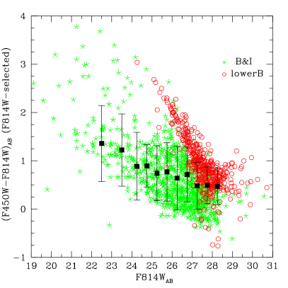
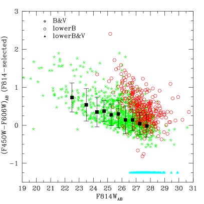
Figure 5: Left panel: (F450W$-$F814W)_AB vs F814W_AB for the F814W-selected sample: in every magnitude bin the median colour is shown, error bars are the standard deviation of the colour distribution. Asterisks represent sources detected both in F450W and F814W bands, while circles mark sources undetected in the F450W band: their colour is a lower limit, defining the F450W_AB magnitude as the $5\sigma$ flux within the isophote on the combined UBVI image. Right panel: (F450W$-$F606W)_AB vs F814W_AB for the F814W-selected sample: asterisks represent sources detected in all F450W, F606W and F814W bands, circles mark sources undetected in the F450W band and triangles sources undetected both in F450W and F606W bands (we assigned to those sources an arbitrary value (F450W$-$F606W)${}_{AB}=-1.25$).

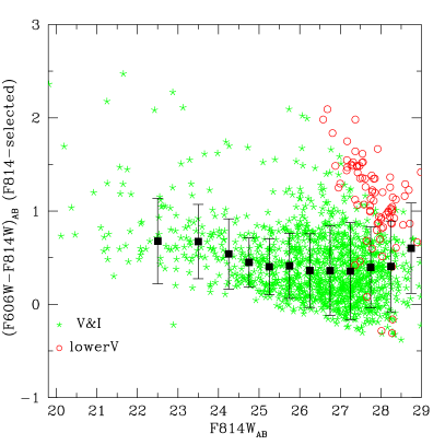
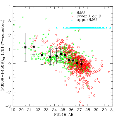
Figure 6: Left panel: (F606W$-$F814W)_AB vs F814W_AB for the F814W-selected sample: asterisks represent sources detected in F606W and F814W bands, circles mark sources undetected in the F606W band. Right panel: (F300W$-$F450W)_AB vs F814W_AB for the F814W-selected sample: asterisks represent sources detected in all F300W, F450W and F814W bands, circles mark sources undetected in the F300W band or F450W and triangles sources undetected both in F450W and F300W bands (we assigned to those sources an arbitrary (F300W$-$F450W)${}_{AB}=2.5$).

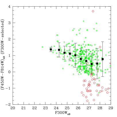
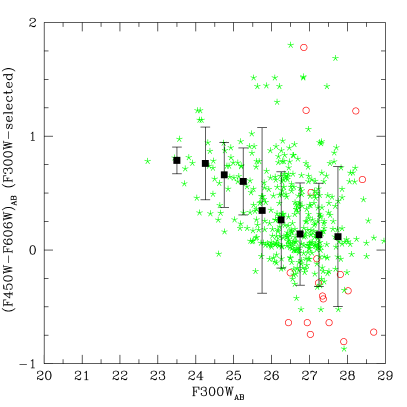
Figure 7: Left panel: (F450W$-$F814W)_AB vs F300W_AB for the F300W-selected sample: in every magnitude bin the median colour is shown, error bars are the standard deviation of the colour distribution. Asterisks represent sources detected in F450W and F814W and F300W bands, while circles mark sources undetected in the F450W or F814W band. Right panel: (F450W$-$F606W)_AB vs F300W_AB for the F300W-selected sample. Asterisks represent sources detected in F450W and F606W and F300W bands, while circles mark sources undetected in the F450W or F606W band.

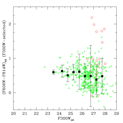
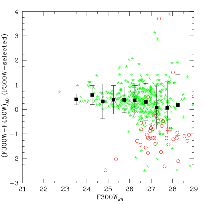
Figure 8: Left panel: (F606W$-$F814W)_AB vs F300W_AB for the F300W-selected sample. Asterisks represent sources detected in F606W and F814W and F300W bands, while circles mark sources undetected in the F606W or F814W band. Right panel: (F300W$-$F450W)_AB vs F300W_AB for the F300W-selected sample. Asterisks represent sources detected in F450W and F300W bands, while circles mark sources undetected in the F450W band.

Figure 9: Fraction of sources in the F814W selected sample with (F450W$-$F606W)_AB bluer than a typical irregular galaxy (Coleman, Wu, Weedman, 1980). The solid line refers to sources detected both in F814W and F450W bands, the dashed line histogram includes also lower limits to magnitudes for sources undetected in the F450W band. The dot-dashed histogram includes also galaxies undetected both in F606W and F450W bands, with lower limits in both magnitudes.

5 Discussion

5.1 Number Counts

Our results show a decreasing slope at redder wavelengths for the whole sample, in good agreement with other works. The very  faint  end  is flatter than 0.2 in F450W_AB, F606W_AB, F814W_AB, while in F300W_AB the slope is steeper.  The  difference  with  Pozzetti  et al. F300W_AB counts is likely due to a different selection of the catalogue: they selected the sample  in  a  red  band  (on  a summed F606W+F814W image) to derive F300W-band counts and used the isophotal magnitude instead of a pseudo-total magnitude. They  assume  that  galaxies  fainter  than F606W${}_{AB}<26$ have approximately a (F300W$-$F606W)_AB color not bluer than the brighter galaxies, not biasing the red-selected sample against very blue objects.

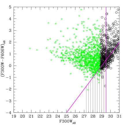
Figure 10: (F300W$-$F606W)_AB color as a function of F300W_AB isophotal magnitude for the F606W-selected sample. Circles represent galaxies with a lower limit in the F300W_AB magnitude and consequently in the (F300W$-$F606W)_AB color. The solid lines represent the (F300W$-$F606W)_AB color of a F606W_AB=29 galaxy (F606W-band limiting magnitude considered by Pozzetti et al. 1998) and the F300W_AB=29.5 limit. The apparent trend towards redder colors for F300W${}_{AB}>$28 is due to the F606W-band limiting magnitude.

In Figure 10 we show the (F300W$-$F606W)_AB color as a function of F300W_AB isophotal magnitude (as Pozzetti et al.) for our F606W-selected sample, within the limiting F606W_AB (i.e. $\approx 30.2$) and for the F300W-selected one (Figure 11). The colors for the F606W-selected sample are obtained as described in Section 4. In order to obtain a sample with characteristics similar to Pozzetti et al. sample, we considered for F300W_AB magnitude the flux within the isophote in the metaimage.

The   solid  oblique  line  represents  the  (F300W $-$F606W)_AB color of a F606W${}_{AB}=29$ galaxy (the F606W-band limiting magnitude of Pozzetti et al.): all galaxies in the hatched area would be not counted since they are fainter than F606W${}_{AB}>29$, the vertical line is the F300W_AB=29.5 limit. The F606W_AB limiting magnitude biases the sample against blue objects, that is the last bins are affected by censored data (see next Section), thus making the (F300W$-$F606W)_AB color appear redder. Considering the bluing trend observed until F300W_AB=29, and the fact that the F606W_AB limiting magnitude biases the sample against blue objects, this implies that F300W-band counts recovered from a red-selected sample are affected by this color bias and consequently by incompleteness in the last bins. The flattening found by other Authors may be mainly caused by the influence of such incompleteness (noise being equally important for faint galaxies, be them at low or high redshift) and not to the “crossing” of the Lyman break.

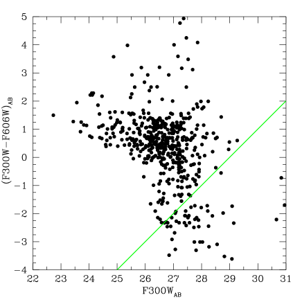
Figure 11: (F300W$-$F606W)_AB color as a function of F300W_AB isophotal magnitude for the F300W-selected sample. The solid line represent the (F300W$-$F606W)_AB color of a F606W_AB=29 galaxy (F606W-band limiting magnitude considered by Pozzetti et al. 1998).

5.2 Colors

As explained in Section 4 we selected two samples: the F814W-selected one should trace the global features of the HDF-S sample and the F300W-selected sample evidencing star-forming galaxies at moderate $z$.

The F814W-selected catalogue has by far the biggest number of sources, so that the number of galaxies with lower limits in the other bands is rather high. We applied a linear fit to the color-magnitude relation by making use of “survival analysis” (Avni et al. 1980, Isobe et al. 1986), in order to avoid uncertainties introduced by the heavy influence of censored data. We applied a linear regression based on Kaplan-Meier residuals. This analysis has suggested an almost flat relation for (F450W$-$F814W)_AB  vs  F814W_AB, (F450W$-$F606W)_AB  vs  F814W_AB and  (F606W$-$F814W)_AB vs  F814W_AB for  F814W${}_{AB}>24$, while (F300W$-$F450W)_AB  vs  F814W_AB did not reach convergence. Smail et al. (1995) noticed a similar tendency on their sample limited at R=27. After an initial bluing the median V$-$R color gets redder, V$-$I gets flat, while R$-$I keeps on following a bluing trend.

This trend may suggest the presence of a flat spectrum population, whose colors seem to saturate but whose contribution is more and more important at faint magnitudes, as confirmed by the rising fraction of galaxies with (F450W$-$F606W)_AB bluer than a typical irregular galaxy. Broadly speaking galaxy colors are dominated by blue sources, as noted by Williams et al. (1996)in the HDF-N, that is the median color is always bluer than typical local samples. The F300W-selected sample shows a very blue (F300W$-$F450W)_AB color, though the relation (F300W$-$F450W)_AB vs F300W_AB seems almost flat. These two features suggest a considerable contribution by flat spectrum sources. Comparing the median (F300W $-$F450W)_AB color with Bruzual & Charlot (1993) and CWW predicted colors, the main contribution may be due to sources with $z>0.5$, while (F450W$-$F814W)_AB, (F606W$-$F814W)_AB and (F450W$-$F606W)_AB are compatible with those of local irregular galaxies.

6 Morphological Number Counts

We performed a morphological analysis of the F814W-selected sample, limited to F814W_AB=25 (Volonteri et al. 2000). We chose a quantitative classification of galaxies morphology, following Abraham et al. (1994, 1996). For each galaxy we measured an asymmetry index ($A$) and a concentration index ($C_{abr}$). The former is determined by rotating the galaxy by 180^∘ and subtracting the resulting image from the original one. The asymmetry index is given by the sum of absolute values of the pixels in the residual image, normalized by the sum of the absolute value of the pixels in the original image and corrected for the intrinsic asymmetry of the background. The concentration index is given by the ratio of fluxes in two isophotes, based on the analysis of light profiles.

We determined number counts by splitting the sample in three bins:  E/S0,  spirals and  irregular/peculiar/ interacting according to our quantitative classification. In every bin the error is estimated as explained in Section 3, considering only contributions due to Poissonian and clustering fluctuation, since according to our simulations the sample at F814W_AB=25 is complete.

In Figure 12 the decrease in differential counts for early-type galaxies at F814W${}_{AB}>$22.5, and the steeper slope for spiral galaxies and irregular/peculiar/interacting ones is clear. They are described by a slope $\gamma_{irr}=0.43\pm 0.05$, $\gamma_{spiral}=0.37\pm 0.05$, we discuss this feature further in Section 7.

Abraham et al. (1996) and Driver et al. (1998) studied the morphological number counts for all galaxies with F814W${}_{AB}<$26.0 detected in the HDF-N. Our results are in agreement with theirs: number counts are dominated by late type galaxies and early type sources show a flat curve. Results for late type galaxies are compatible with a strong evolution in number or with a non negligible fraction of sources being at moderate redshift, as suggested also by the analysis of colors. This result fits in Marzke et al. (1997) findings about the LF of galaxies as a function of their color: the slope of the LF faint end is steeper at low luminosities for the bluest galaxies ($M^{*}_{B}\approx-19.4$, $\alpha<-1.7$ for galaxies bluer than B$-$V=0.4). Actually by integrating this LF, within $z=0.5$, the number density of galaxies bluer than an Irregular galaxy is compatible with the number found in our sample. The flattening of the curve for early type sources may be due to a decrease in density at higher redshift of elliptical galaxies, but it is also expected by the $\alpha>-1$ slope of the LF of early type galaxies (e.g. Marzke et al. 1998). Number counts models nevertheless show that an $\alpha>-1$ LF does not account for such a steep decrease (Figure 12).

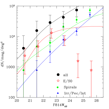
Figure 12: Morphological number counts: early type galaxies are shown as circles, spiral galaxies are shown as pentagons and peculiar galaxies as squares, the total counts are shown as filled circles. Late type galaxies have steep slopes, $\gamma_{irr}=0.43\pm 0.05$, $\gamma_{spiral}=0.37\pm 0.05$. Lines show number counts model for a flat cosmological model ($q_{0}=0.5$, $H_{0}=50$ km s^-1 Mpc^-1, $\Lambda=0$) and the LF of Marzke et al. (1998): the models by types are obtained by keeping the parameters which best fit the total counts.

Brinchmann et al. (1998), Im et al. (1999) and Driver et al. (1998) studied the redshift distribution for different morphological types in deep surveys. Brinchmann et al. (1998) analyzed 341 galaxies at $z<1$ from the Canada-France Redshift Survey (CFRS, Lilly et al. 1995, limited at F814W_AB=22.5), and Autofib/Low-Dispersion Survey Spectrograph (LDSS, Ellis et al. 1996, limited at $b_{j}=24$). They find the distribution of elliptical galaxies peaked at $z\approx 0.5$, while spiral galaxies have a shallow distribution and the excess of peculiar sources begins at $z\approx 0.4$. According to their conclusions, the number of regular galaxies is compatible with a passive evolution model, while the excess of peculiar ones suggests an active luminosity evolution and-or number evolution. Im et al. (1999) for a sample of 464 galaxies limited at I$=21.5$ do agree with Brinchmann et al. (1998). Driver et al. (1998) analyzed HDF-N sources, with photometric redshifts, and underline the excess both in spiral galaxies at $z=1.5$ and irregulars at $z>1$, suggesting number evolution and passive evolution for dwarf LSBG at $z<1$ giving the density of irregular galaxies at low redshift.

7 Constraining the Redshift of Galaxies from Photometric Data

In a deep survey, such as the HDF-S, the contribution of low redshift foreground sources should be disentangled from the contribution of high redshift ones. We first tried to split the two populations with very simple considerations, regarding galaxy colors and counts.

We compared colors of HDF-S galaxies with those predicted by CWW spectra and  by  synthetic  spectra  of Bruzual & Charlot (1993, BC hereafter). While BC account for evolution, the  CWW  spectra  take  into  account $K-corrections$. In Figures 13-14 apparent colors from CWW and BC are shown. We limited our analysis at $z<2$ to avoid relying too much on the UV part of spectral energy distributions which has a strong influence at higher redshift.

By comparison with colors predicted by CWW or BC spectra, the observed very blue galaxies (med(F450W${}_{AB}-$ F606W_AB) = 0.06,  med(F606W${}_{AB}-$ F814W_AB) = 0.24) are compatible with two very different ranges in redshift: $z<0.2$ or $z>1.5$ (and perhaps beyond our analysis limit). The slope of morphological number counts is in good agreement with this hypothesis, assuming that most of the faint late type galaxies are at moderate redshift. In the hypothesis of the moderate redshift population ($z\leq 0.2)$ we computed number counts as a function of optical colors, which should reflect rest-frame colors for this range in z. We divided the F814W-selected sample in a “red” subsample, composed by sources redder than the median colour of the sample (F450W${}_{AB}-$ F606W_AB=0.45) and a “blue” subsample of the remaining sources. We limited our analysis at F814W_AB=26, where the catalogue is complete, according to our simulations.

The curve for blue sources is much steeper than the red one, as shown in Figure 15. We estimated $\gamma_{blue}\sim 0.49\pm 0.01$. This value is therefore compatible with the previous hypothesis, that a non negligible fraction of the blue galaxies may have a moderate redshift, contributing with an almost Euclidean slope to the counts or with number evolution, with very faint galaxies merging at high redshift. However we cannot rule out the hypothesis that such a steep slope can be due to earlier-type evolving galaxies which move into the blue sample at high redshift. In such a case the steep counts described by the faint blue sample would not require a significant rate of merging to be justified.

Figure 13: (F450W$-$F606W)_AB color from Coleman, Wu e Weedman (1980) spectra, convolved with HST filter responses. $K-corrections$ have been applied, but no evolution has been considered. The solid line refers to irregular galaxies, the dot-dashed line to disk galaxies, the dashed line to ellipticals.

Figure 14: As in Figure 13 but considering Bruzual & Charlot (1993) of synthetic stellar evolution spectra, with a Miller-Scalo IMF. The star formation rate is exponentially decaying with timescales 1 Gyrs and 5 Gyrs for E and Sb respectively, and is constant for Im.

In order to check the low-redshift solution we compared the characteristics of those galaxies to the predictions of a local luminosity function. The brightest of the very blue sources would have $M_{B}\geq-18$ if placed at $z=0.2$  (assuming  $H_{0}$=50 km s^-1 Mpc^-1   and a (F450W$-$F814W)_AB=1).

Figure 15: Number counts for blue and red galaxies (i.e. (F450W$-$F606W)${}_{AB}<0.45$ or vice versa). The blue sources have a very steep slope ($\gamma_{blue}\sim 0.49\pm 0.01$), while red sources have a shallower end.

Considering the local luminosity function (LF) of blue galaxies as estimated by Marzke et al. (1997), described by $\alpha=-1.8$ and $M^{*}_{B}\approx-$19.5 and integrating within $z=0.2$ and $M_{B}=-$18, the number density found is compatible with all very blue galaxies (i.e. galaxies with (F450W$-$F606W)_AB and (F606W$-$F814W)_AB bluer than a local Irregular galaxy) being at such a low redshift. The first raw technique used to constrain the redshift of sources suggests that a high fraction of faint galaxy is composed by low redshift ($z<0.2$) sources, nevertheless the “high redshift solution” is not ruled out, since steep counts may be due also to merging and our color analysis is very naive.

We then made our analysis better by means of the photometric redshift technique. We computed photometric redshifts for the galaxies in the F814W catalogue by means of the public code hyperz (Bolzonella et al. 2000). The method basically consists in a comparison between the observed magnitudes and the photometry expected from a set of Spectral Energy Distributions (SEDs). The efficiency of the method relies on the presence of strong spectral features, in particular the $4000$ Å  break and the Lyman break for galaxies at high redshift. To reduce the uncertainties estimating $z_{phot}$, the set of filters must be able to identify these characteristics, spanning a wide range of wavelength. The photometric redshift $z_{phot}$ is computed by a $\chi^{2}$ minimization, considering the whole set of possibilities with different combinations of the involved parameters.

In this procedure we decided to use the SEDs built from the Bruzual & Charlot’s synthetic library (GISSEL98, Bruzual & Charlot 1993), rather than the observed mean local spectra by CWW, because tests on HDF-N indicate a slightly lower dispersion at $z<2$. In any case, CWW spectra lead to not very different conclusions. Hence, we selected 5 spectral types, characterized by different star formation rates, matching the observed colors of the morphological galaxy sequence; a subsample of ages allowed by the GISSEL library is also considered. Moreover, we took into account the possible presence of dust applying the reddening law by Calzetti et al. (2000) for different values of $E_{B-V}$. The flux decrement produced by intervening neutral hydrogen is computed following the recipe by Madau (1995). Only spectra with solar metallicity are considered here, because the metallicity can be regarded as a secondary parameter.

The accuracy of photometric redshift estimate obtained from the considered set of filters can be studied by means of simulations on synthetic catalogue.

Some degeneracy can be found (Bolzonella et al., 2000), with a non negligible part of galaxies lying at $z\simeq 1$ – $2.4$ incorrectly located at low redshift. These galaxies show frequently a probability function with several comparable peaks, at low and high $z$, due to the degeneracy in the parameter space. Near infrared data can in principle avoid these uncertainties. Nonetheless, also with the available set of filters, we can guess that the objects with $z_{phot}\gtrsim 1$ really belong to this redshift, because high-$z$ objects are rarely misidentified as low-$z$ galaxies.

Photometric redshifts for our catalogue indicate that all very blue galaxies are at $z_{phot}\geq 1$ (med($z_{phot}$)=1.6). This feature, along with their steep slope (see Section 5), suggests a high merging rate for galaxies at $z_{phot}\geq 1$. Vice versa very red sources have a shallower redshift distribution (med($z_{phot}$)=0.6), though at F814W${}_{AB}>25$ most sources have a high redshift.

Similarly, at F814W${}_{AB}<$25, late type galaxies have a higher median redshift (med($z_{phot}$)=1.1) than  early  type  ones (med($z_{phot}$)=0.6) and the redshift distribution (Figure 16) is similar to Driver et al. (1998) one, though the number of sources at $z_{phot}>1.5$ is lower. There is a point to be emphasized about redshift distributions and morphological types: the detection of galaxies at high redshift is seriously biased against elliptical galaxies because of $K-corrections$ in the F814W-band. At $z\approx 1$, early type galaxies have $K-corrections$ ($\approx 1$ mag) greater than late type $K-corrections$, making them fainter. It means that a cut in apparent magnitude, such as F814W${}_{AB}<$25, biases the sample toward galaxies with lower $K-corrections$. To skip this problem, we tried to select a volume-limited sample, based on our photometric redshifts. When selecting all galaxies with $z_{phot}\leq 1$, we found only 15$\%$ to be with F814W${}_{AB}<$25, that is with a reliable morphological classification according to our method. Vice versa it means that a cut off in apparent magnitude does not offer a fair sample for a redshift distribution of the different morphological types.

Probably also the apparent decrease in early-type galaxies number counts, as shown in Figure 12, is due to this bias.

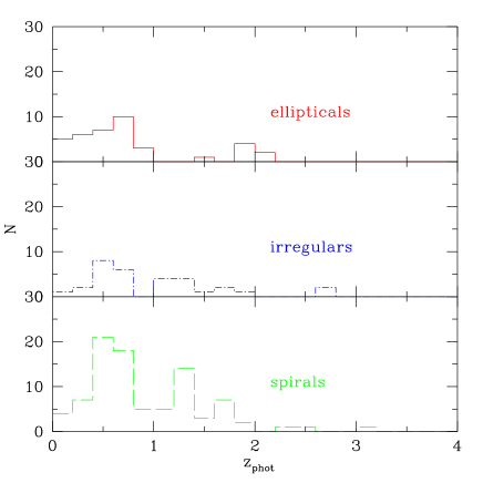
Figure 16: Morphological redshift distributions for F814W${}_{AB}<$25.

We compared our number counts with different models, by using galaxy counts models by Gardner (1998). We adopted a flat cosmological model ($q_{0}=0.5$, $H_{0}=50$ km s^-1 Mpc^-1) in all models. We used the luminosity function of Marzke et al. (1998) both considering a single Schechter function for all morphological types and three different Schechter fits for elliptical, spiral and irregular galaxies. Our counts are best fitted by considering three LFs, luminosity evolution and a moderate merging (Figure 17) consistent with our interpretations. The merging rate in Gardner (1998) follows Rocca-Volmerange & Guiderdoni (1990) with number evolution parameterized as $\phi^{*}\propto(1+z)^{\eta}$ in the Schechter fit to the LF, and in order to conserve the luminosity density, $L^{*}\propto(1+z)^{-{\eta}}$; $\eta$ is a free parameter. Good fits to our data are obtained with $\eta\leq 0.5$ in the case of three LFs for the cosmological parameters considered.

Figure 17: Number counts models compared to various counts obtained in literature and in this work. All models adopt Marzke et al. (1998) luminosity function, the dot-dashed line refers to three Schechter fits for elliptical, spiral and irregular galaxies with no evolution, the solid line uses the same LFs with luminosity evolution and a moderate merging, the dotted line is obtained by using a single Schechter fit without evolution, the short dashed considers luminosity evolution and the long dashed both luminosity evolution and strong merging for the same LF.

8 Summary and Conclusions

The HDF-S represents a unique opportunity for the study of  faint  galaxies  up to  now,  both  for  its  depth (F814W${}_{AB,lim}\approx 29$ for detection and F814W${}_{AB,lim}\approx 27$ for completeness) and spatial resolution (FWHM$\approx$0.2 arcsec). We presented here colors and number counts of HDF-S galaxies, along with number counts determined by splitting the sample considering the morphology and the colors of the galaxies. We also analyzed the photometric data to constrain the redshift of HDF-S galaxies, and determine the contribution of different redshift populations to the counts. The main results are the following:

• the number-counts relation has an increasing slope up to the limits of the survey in all four bands. The slope is steeper at shortest wavelengths;

• the number counts model which best fits our data is obtained by considering three different Schechter functions for elliptical, spiral and irregular galaxies (Marzke et al. 1998), luminosity evolution and a moderate merging ($\eta<0.5$);

• optical colors show that the sample contains a high fraction of galaxies bluer than local sources, for instance at F814W${}_{AB}>27$ about $50\%$ of sources have (F450W$-$F606W)_AB bluer than a typical local irregular galaxy;

• after an initial blueing trend the color-magnitude relation gets flat, suggesting a color-saturation due to a strong contribution of a flat spectrum population in the faintest bins;

• morphological number counts ( F814W${}_{AB}<25$) are dominated by late type galaxies ($\gamma_{irr}=0.43\pm 0.03$, $\gamma_{spir}=0.37\pm 0.03$), while early type galaxies show a steep decrease in the faintest bin;

• photometric redshifts of our sample galaxies show that the galaxies contributing with a steep slope to the number counts have $z_{phot}\gtrsim 1$, suggesting a moderate merging;

• morphological redshift distributions and number counts are biased against elliptical galaxies when using an apparent magnitude cut-off.

Our number counts are in good agreement with previous results, except for the F300W-band number counts in the HDF-N.

We do not see a flattening in F300W-band number counts, limiting our analysis at F300W${}_{AB}<$26.5. A steep F300W-slope may be explained both with a high fraction of low redshift galaxies or with merging or a mixture of them. In the former case, intrinsically faint, low redshift galaxies, imply a steep faint end slope of the LF in the F300W-band ($\alpha\approx-2$) in the latter case we emphasize that if merging is the reason of the steep F300W-band counts, it would take place at $z<2$ since the Lyman break prevents us from detecting galaxies in the F300W-band at higher redshift. A way of detecting merging and hence to check the validity of the hierarchical model, could be in principle the study of the evolution with look-back time of some structural parameters of galaxies, such as their intrinsic size.

Morphological number counts are in agreement with previous results, as well as the morphological redshift distributions. The morphological classification is, however, possible only for bright galaxies. The cut in apparent magnitude biases the sample against early-type galaxies, due to their large $K-corrections$. A correct test implying morphological classification should be done using K-band data (an extension of the test proposed by Kauffmann & Charlot, 1998) or a volume-limited sample, with morphology determined from spectra. Extracting a volume-limited sample from a magnitude limited survey does not fit the goal since at $z\lesssim 1$ almost 80$\%$ of the galaxies are too faint for a reliable morphological classification from imaging.

- (1) Abraham, R. G., Valdes, F., Yee, H. K. C., van den Bergh, S., 1994, ApJ, 432, 75
- (2) Abraham, R. G., van den Bergh, S., Ellis, R, S., Glazebrook, K., Santiago, B. X., Griffiths, R. E., Surma, P., 1996, ApJS, 107, 1
- (3) Arnouts, S., D’Odorico, S., Cristiani, S., Zaggia, S., Fontana, A., Giallongo, E. 1999, A&A, 341, 641
- (4) Avni, Y., Soltan, A., Tanambaum, H., Zamorani, G. 1980, ApJ, 235, 694
- (5) Bahcall J. N. & Soneira R. M. 1981, ApJS 47, 357
- (6) Barger A. J., et al. 1999, AJ 117, 102
- (7) Baugh C. L., Cole S., Frank C. S. 1996, MNRAS 283, 1361
- (8) Benítez N., et al. 1999, ApJ 515, L65
- (9) Bertin, E., Arnouts, S., 1996, A&AS, 117, 393
- (10) Bolzonella M., Miralles J.M. & Pello’ R., 2000, A&A submitted, astro-ph/0003380
- (11) Brainerd, T. G., Smail, I. R., Mould, J. r. 1994, BAAS, 185, 114.06
- (12) Broadhurst T. J., Bowens R. J. 2000, ApJ 530, 53
- (13) Bruzual, A.G., Charlot, S., (BC) 1993, ApJ, 405, 538
- (14) Brinchmann, J., et al., 1998, ApJ, 499, 112
- (15) Calzetti, D., Armus, L., Bohlin, R.C., Kinney, A.L., Koornneef J., ApJ, 533, 682
- (16) Coleman, G.D., Wu, C.C., Weedman, D.W., (CWW) 1980, ApJS, 43, 393
- (17) Colless, M., Ellis, R.S., Taylor, K., Hook, R., 1990, MNRAS, 244, 408
- (18) Colless, M., Schade, D., Broadhurst, T., Ellis, R.S., 1994, MNRAS, 267, 1108
- (19) Cowie, L.L., Lilly, S.J., 1989, ApJ, 336, L41
- (20) Cowie, L. L., Gardner, J. P., Hu, E. M., Songaila, A., Hodapp, K. W., Wainscoat, R. J. 1994, ApJ, 434, 114
- (21) Daddi et al. A&A submitted, astro-ph/0005581
- (22) Driver, S. P.; Fernandez-Soto, A.; Couch, W. J.; Odewahn, S. C.; Windhorst, R. A.; Phillips, S.; Lanzetta, K.; Yahil, A., 1998, ApJ, 496L, 93
- (23) Djorgovski, S., et al. 1995, ApJ, 438, L13
- (24) Ellis, R.S., Colless, M., Broadhurst, T., Heyl, J., Glazebrook, K., 1996, MNRAS, 280, 235
- (25) Ellis, R.S.,1997, ARA&A 35, 389
- (26) Fontana, A. et al. 1999, A&A, 343, L19
- (27) Fontana A., et al. 1999, MNRAS 310, L27
- (28) Franceschini A., et al. 1998, ApJ 506, 600
- (29) Gardner, J.P., Sharples, M.R.. Frenk, C.S., Baugh, C.M., Carrasco, B.E., 1996, MNRAS, 282, L1
- (30) Gardner, J.P., 1998, PASP, 110, 291
- (31) Griffiths R. E., et al. 1994, ApJ 435, L19
- (32) Hogg, D.W., Pahre, M.A., McCarthy, J.K., Cohen, J.G., Blandford, R., Smail, I., Soifer, B.T, 1997, MNRAS, 288, 404
- (33) Im, Myungshin; Griffiths, Richard E.; Naim, Avi; Ratnatunga, Kavan U.; Roche, Nathan; Green, Richard F.; Sarajedini, Vicki L., 1999, ApJ, 510, 82
- (34) Isobe, T., Feigelson, E. D., Nelson, P. I. 1986, ApJ 306, 490
- (35) Jones, L.R., Fong, R., Shanks, T., Ellis, R.S., Peterson, B.A., 1991, MNRAS, 249, 481
- (36) Kauffmann G., 1996, MNRAS 281, 487
- (37) Kauffmann, G., Charlot, S., 1998 MNRAS 297L
- (38) Koo, D.C., 1986, ApJ, 311, 651
- (39) Koo D. C., Kron R. G., 1992, ARA&A, 30, 613
- (40) Le Fèvre O., et al. 2000, MNRAS 311, 565
- (41) Lilly, S.J., Cowie, L.L., Gardner, J.P., 1991, ApJ, 369, 79L
- (42) Lilly, S. J., Le Fèvre, O., Crampton, D., Hammer, F., Tresse, L. 1995, ApJ, 455, 50
- (43) Lilly S. J., et al. 1998, ApJ 500, 75
- (44) Madau, P., 1995, ApJ, 441, 18
- (45) Marzke, R.O., Da Costa, N.L., Pellegrini, P.S., Willmer, C.N.A., Geller, M.J., 1998, ApJ, 503, 617
- (46) Marzke, Ronald O.; da Costa, L. Nicolaci, 1997, AJ, 113, 185
- (47) Mendez, R.A., Guzman, R. 1998, A&A, 333, 106
- (48) Metcalfe, N.; Shanks, T.; Fong, R.; Jones, L. R., 1991, MNRAS, 249, 498
- (49) Metcalfe, N., Shanks, T., Fong, R., Roche, N., 1995, MNRAS, 273, 257
- (50) Moustakas, L. A., Davis, M., Graham, J. R., Silk, J., Peterson, B. A., Yoshii, Y., 1997, ApJ, 475, 445
- (51) Neushaefer L. W., Im M., Ratnatunga K. U., Griffiths R. E., Casertano S., 1997, ApJ 475, 29
- (52) Oke, J.B. 1974, ApJS, 27,21
- (53) Pozzetti, L., Madau, P., Zamorani, G., Ferguson, H.C., Bruzual, A. 1998, MNRAS , 298,1133
- (54) Rocca-Volmerange, B., & Guiderdoni, B. 1990, MNRAS, 247, 166
- (55) Roche, N., Shanks, T., Metcalfe, N., Fong, R. 1996, MNRAS, 280, 397
- (56) Schade D. J., Lilly S. J., Crampton D., Hammer F., Le Fèvre O., Tresse L,. 1995, ApJ 451, L1
- (57) Saracco, P., D’Odorico, S., Moorwood, A., Buzzoni, A., Cuby, J.G., Lidman, C., 1999, A&A, 349, 751
- (58) Smail, I., Hogg, D.W., Yan, L., Cohen, J.G., 1995, AJ, 449, L105
- (59) Tyson, J.A., 1988, AJ, 96,1
- (60) van den Bergh, S., Abraham, R.G., Ellis, R.S., Tanvir, N.R., Santiago, B.X., Glazebrook, K., 1996, AJ, 112, 359
- (61) Volonteri, M., Saracco, P., Chincarini, G., 2000, A&A in press, astro-ph/0005204
- (62) Williams R.E., Blacker, B., Dickinson, M., Van Dike Dixon, W., Ferguson, H.C., Fruchter, A.S., Giavalisco, M., Gilliland, R.L., Heyer, I., Katsanis, R., Levay, Z., Lucas, R.A., McElroy, D.B., Petro, L., Postman, M., 1996, AJ, 112, 1335
- (63) Zepf S. E., 1997, Nature 390, 377