Noise-driven evolution in stellar systems:
A universal halo profile

Abstract

Using the theory describing the evolution of a galaxy halo due to stochastic fluctuations developed in the companion paper, we show that a halo quickly evolves toward the same self-similar profile, independent of its initial profile and concentration. The self-similar part of profile takes the form of a double power law with inner and outer exponents taking the values near $-1.5$ and $-3$ respectively. The precise value of the inner exponent depends on the magnitude and duration of the noisy epoch and most likely on form of the inner profile to start. The outer exponent is the result of evolution dominated by the external $l=1$ multipole resulting from the inner halo’s response to noise.

Three different noise processes are studied: (1) a bombardment by blobs of mass small compared to the halo mass (‘shrapnel’); (2) orbital evolution of substructure by dynamical friction (‘satellites’); and (3) noise caused by the orbit of blobs in the halo (‘black holes’). The power spectra in the shrapnel and satellite cases is continuous and results in the double power law form, independent of initial conditions. The power spectrum for black holes is discrete and has a different form with a much slower rate of evolution. A generic prediction of this study is that noise from transient processes will drive evolution toward the same double power law with only weak constraints on the noise source and initial conditions.

1 Introduction

There is considerable evidence from numerical experiments that haloes formed in CDM simulations are well-approximated by two-component power law profiles of the form $\rho\propto r^{-\gamma}(1+r/r_{s})^{\gamma-3}$ or $\rho\propto r^{-\gamma}(1+(r/r_{s})^{3-\gamma})^{-1}$. The first form was presented by Navarro, Frenk & White (1997, hereafter NFW) based on a suite of simulations with different initial density fluctuation spectra and cosmological parameters. They suggest $\gamma=1$ is the universal exponent. Moore et al. (1998) find that the form of the inner profile ($\gamma$) is resolution dependent. With $3\times 10^{6}$ particles within the virial radius, this group finds $\gamma=1.4$. Jing & Suto (2000) find that the inner slope is not universal but varies depending on environment; they find $\gamma=1.5,1.3$ and $1.1$ for galaxy-, group-, and cluster-mass haloes, respectively. Besides issues of n-body resolution and methodology, attempts to explain the discrepancy of these collisionless simulations and astronomical observations include new laws of physics (Spergel & Steinhardt 2000) and the effects of gas dissipation (Tittley & Couchman 1999, Frenk et al. 2000, Alvares, Shapiro & Martel 2000).

The suggestion of some sort of universal profile and more generally the physics of dissipationless collapse or violent relaxation has a long history. The general problem of stellar dynamics in the presence of large fluctuations is very difficult and much of this focuses on first-principle forms for the phase-space distribution. The companion paper approaches this problem as near-equilibrium evolution in a noisy environment (see Weinberg 2000, Paper 1, for a review of recent theoretical work on this subject). Here we apply the theory from Paper 1 to follow the evolution of haloes with a number of different concentrations and shapes. The near-equilibrium restriction allows development of a solvable evolutionary equation given some initial condition. We find that the profile rapidly assumes a double power law form with $\gamma\approx 1.5$ independent of the initial model. So in the presence of noise, a quasi-self-similar profile does appear and in this sense represents the near-equilibrium limit of violent relaxation. The inner power-law profile evolves slowly if the noise is applied over long periods. This evolution of the inner halo may depend on the details of the central initial conditions (e.g. power-law cusp or core) and possibly the noise source. Investigation of this issue is underway.

The plan for this paper is as follows. The basic principles from Paper 1 are described and reviewed in §2 followed by a description of the noise models in §3. Although we choose several particular astronomical scenarios to derive particular noise spectra, the resulting halo profiles are insensitive to the shape of the power spectrum for noise due to transient perturbations; the dynamics behind this finding is described. We also consider an example of non-transient noise source, a halo of massive black holes. This case does not result in the double power law form and leads to much weaker evolution overall. The resulting halo profiles are described in §4 followed by a discussion in §5 and summary in §6.

2 Physics of noise-driven evolution

Let us begin by considering a perturbation to a galaxy halo. For example, a dwarf passing through the halo. The halo responds with a wake whose form depends on the halo profile, perturber velocity and minimum impact parameter (the dynamics for a single encounter has been considered in detail by Vesperini & Weinberg 2000). The gravitational attraction of the halo wake and the interloping dwarf exchanges energy and angular momentum between the two. This new momentum is deposited (or removed) in the dark matter halo at the location of the wake. After the dwarf is gone, the halo will adjust its profile to reachieve equilibrium. As long as the wake is relatively small, many such transient encounters may be in progress simultaneously without mutual interaction. We may now ask the question: can we compute the mean evolution after many such encounters without resorting to simulating an ensemble of encounters at high resolution?

The answer to this question motivates the development of an evolution equation that may be solved numerically but without simulation (see Paper 1). The resulting evolution equation takes the Fokker-Planck form, similar to the kinetic equation used in studying globular cluster evolution, although the details are cumbersome and the approach somewhat different. The shape of the wake (or ensemble of wakes for different types of encounters) will determine the diffusion coefficients and subsequently the shape of the evolving halo profile.

This shape of the wake is key to understanding how noise can drive a self-similar evolution. Both Weinberg (1998) and Vesperini & Weinberg (2000) illustrate an important fact in the dynamics of hot collisionless systems: a halo has a low-order $m=1$ and to a lesser extent $m=2$ weakly damped mode. Because these modes damp slowly, they tend to dominate the wake. Weinberg (1998 and subsequent work) shows that the scale of $m=1$ mode is proportional to the characteristic radius of a halo profile. The interaction between the wake and the disturbance changes the actions of the orbits in the modal excitation. In the case of the fly-by example above, the energy of these orbits tend increase over the range of the mode and this modifies the halo profile. The new characteristic radius then governs the size and shape of subsequent modal excitations. The direct calculation shows that this process rapidly become self-similar and results in a new power law slowly working its way out in the halo. Although it was not obvious a priori that this would be the result of the noise-driven evolution, we will see that it describes the numerical solutions in §4.

We consider two general types of noise perturbations in this paper: transient and quasi-periodic perturbations. These cover the types of astronomical scenarios that are likely to be important. In addition to the dwarf fly-by in the example above and orbital decay which will be considered explicitly in this paper, a transient event might be a damping disk density wave or bar instability. Astronomically relevant quasi-periodic perturbations result from something orbiting in the galaxy halo and such a halo of super massive black holes whose individual masses are too small for dynamical friction to be significant.

For a transient perturbation, the relative distribution of power over all frequencies will depend on its details. However, the continuous spectra perturbations will nearly always have some power near the frequencies of weakly damped modes. In the halo case, the response is dominated by the weakly damped $m=1$ mode by at least an order of magnitude. Therefore, no matter what shape the frequency spectrum takes, the response will be similar. This, together with description of self-similar evolution above, is at the root of the surprising claim that noise can result in a nearly universal profile, independent of its source.

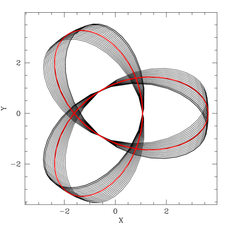
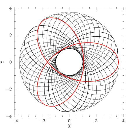
For a quasi-periodic perturbation, the power will be at discrete frequencies. Each dark matter orbit only changes if driving frequencies couple to its natural orbital frequencies. For orbiting point masses, these resonances must have zero frequency in order to apply a torque; in other words, the resonant orbits are closed orbits. If the perturber orbit is not closed, then over a long period of time, its density will be axisymmetric and can not result in angular momentum and energy exchange (see Fig. 1 for an pictorial example). For a physically plausible halo, there will be no closed orbits at orders $l=1$ and $2$ for the following reasons. Our closed orbit condition is $n\Omega_{1}+m\Omega_{2}=0$ where $\Omega_{1}$ and $\Omega_{2}$ are the radial and azimuthal orbital frequencies. The ratio $\Omega_{1}/\Omega_{2}$ ranges from 1 to 2 in most profiles. For $l=1$, we have $|m|\leq 1$ and a closed orbit for $m=1$ will only then obtain for a point mass potential. Similarly, for $l=2$, $|m|\leq 2$ and a closed orbit for $m=2$ will only then obtain at the centre of a homogeneous core. Both of these conditions are represented by a vanishingly small number of orbits and therefore there are no resonant contributions by internally orbiting point masses for harmonics with $l<3$.

(a) Close to resonance

(b) Off resonance

Figure 1: Orbit close to zero-frequency low-order resonance ($n=-3,m=2$): (a) very close to resonance; (b) slightly off resonance. The heavy curve marks the closed resonant orbit.

3 Models and noise sources

We consider three classes of initial profiles: King models (1966) with concentrations $c$ between 0.67 and 1.5, Plummer models (e.g. Binney & Tremaine 1987), and models of the form:

$$\rho\propto{1\over(r+\epsilon)^{\gamma}}{1\over(r+1)^{\beta-\gamma}}.$$ (1)

Solution of the evolution equation requires repetitive integration of the distribution function to derive the density, mass and potential profiles. For this reason, the dynamic range of cuspy models present considerable numerical challenge and are not considered here, unfortunately. However, the instantaneous fluctuation spectrum in models with and without cores exhibit strong enhancement due to $l=1$ modes (see Weinberg 1998); this suggests that qualitative behavior here will be similar as well since the underlying physical process is the same. The model described in equation (1) has most of the features of popular cusp models but gets around numerical difficulties of divergent distribution phase-space distribution functions for carefully chosen values of small but non-vanishing values of $\epsilon$. It remains a possibility that an initial cusp may effect the sense of the evolution of the inner power law. We will extend the development to study this case in detail in a later paper. Here, we focus on the rapid approach to a self-similar form ouside of the core.

We consider three specific noise sources: (1) transient noise due to blobs moving on rectilinear trajectory (‘shrapnel’ model); (2) transient noise due to substructure on decaying halo orbits due to dynamical friction (‘satellite’ model); and (3) quasi-periodic noise due to blobs orbiting within the halo (‘black hole’ model). The derivation of moments for the evolution equation can be found in §4 of Paper 1. For all noise sources, the amplitude for a single event is proportional to the square of the mass in the perturbation since the net change in conserved quantities is second order. From the form of the collisional Boltzmann equation, the evolutionary time scale is inversely proportional to amplitude of the collision term. This allows easy scaling of the results derived here for each noise source described below. We will set some fiducial parameters for results quoted in §4 and give the scaling formula for the amplitudes so that the time scales can be easily derived for other scenarios.

For the shrapnel model, the overall amplitude for the process is also proportional to the bombardment rate. We assume that the flux of shrapnel is uniform so that the distribution impact parameters $b$ is proportional to $b$. Soon after formation, one expects encounters to be more numerous so we adopt a fiducial rate of 10 encounters per gigayear inside of 50 kpc, each with a mass of 0.003 halo masses. Scaling to our Galaxy, our fiducial shrapnel has 15% of the LMC mass. The trajectories have constant velocity chosen to be $\sqrt{2}$ times the peak halo circular velocity. However, the results are nearly unchanged if the incoming velocity is increased or decreased by a factor of two and so this is not a sensitive assumption.

For the satellite model, we assume a halo’s worth of satellites of a given mass assimilating within 1 Gyr. Because the amplitude is proportional to the square of the satellite to halo mass ratio but the number of satellites is proportional to the inverse of this ratio, the overall amplitudes scales as the satellite to halo mass ratio. This scaling is roughly consistent with the substructure distribution described by Moore et al. (1999). For smaller numbers of satellite per halo, the overall amplitude can be multiplied by the desired factor which lengthens the time scale proportionately. The noise spectrum results from following the orbital decay of a satellite of given mass ratio by direct integration of the equations of motion of an initially circular orbit at a radius enclosing 95% of the halo mass. The drag force is computed using Chandrasekhar’s formula with $\ln\Lambda=8$; this value provides a good match to substructure simulation (Tormen et al. 1998). Although the power spectrum is computed for the full orbital decay of the satellite, the amplitude is diminished by the fraction of satellites with orbits that can fully decay in one gigayear. Mass loss from the satellite is not included.

In the case of the black hole model, the amplitude of the noise also is proportional to the square of the perturber mass for a single perturber. However, the amplitude is also proportional to number of perturbers. For a fixed fraction in black holes, the number is then inversely proportional to the black hole mass. Altogether, then, the amplitude is directly proportional to the perturber mass and the fraction of the halo represented by the perturber mass. For our fiducial example, we assume a halo fully populated by $10^{6}$ solar-mass black holes (Lacey & Ostriker 1985).

The scaling and fiducial parameters for all of these cases is summarized in Table 1.

Table 1: Scaling and fiducial parameters

Shrapnel model: $A=A_{o}(R_{enc}/R_{enc\,0})(m_{enc}/m_{enc\,0})^{2}$
$R_{enc}$	Number of encounters within 50 kpc per Gyr	10
$m_{enc}$	Relative mass of shrapnel (units of halo mass)	0.03
Satellite model: $A=A_{o}N_{Halo}(m_{sat}/m_{halo})^{2}(\ln\Lambda/8.0)^{2}$
$m_{sat}/m_{halo}$	Satellite to halo mass ratio	0.01, 0.03, 0.05
$N_{halo}$	Number of satellites accreting per Gyr	$m_{halo}/m_{sat}$
Black hole model: $A=A_{o}(f_{bh}/f_{bh\,0})(n_{bh}/n_{bh\,0})$
$n_{bh}$	Relative mass of body (units of halo mass)	$10^{6}$
$f_{bh}$	Fraction of halo in lumps	$1.0$

4 Resulting halo profiles

The evolution equation, a Boltzmann equation with a Fokker-Planck-type collision term, is derived in Paper 1. To simplify the numerical solution, the full equation is isotropized by averaging over angular momentum to leave an equation for the phase-space distribution function in energy $E$ and time $t$ (see Appendix §A and Paper 1). The Fokker-Planck equation is solved on a grid as described in Appendix §B. The energy variable $E$ is remapped to better populate the centre and outer halo with grid points. This new mapping variable $x=x(E)$ is monotonic in energy and described in Appendix §C.

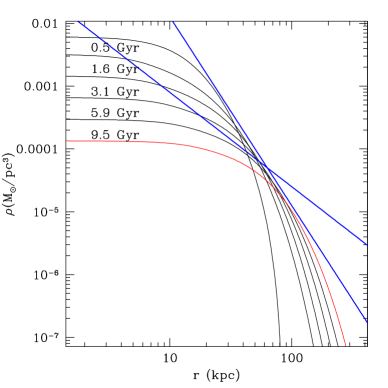
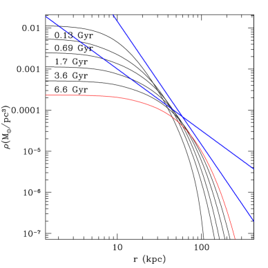
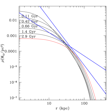
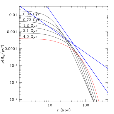
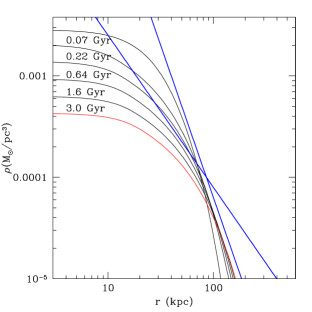
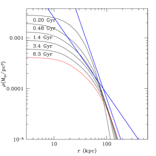
Figure 2 shows the evolution of four different initial models under shrapnel noise. The radial scaling is chosen to place the initial half-mass radius at approximately 50 kpc. The main features are as follows:

1. In all cases, there are two distinct evolutionary phases: (1) a transient readjustment to a double power law profile; (2) slow, approximately self-similarly evolution of the double power law profile. The transition period will be described in more detail below.

2. The asymptotic outer power law exponent is -3. The profile continues to approach the -3 form at increasing radius as the evolution continues.

3. The inner power law exponent is approximately -1.5 after the transient readjustment phase and slowly decreases thereafter. For example, after 1.9 Gyr in Panel (a) in Figure 2, the inner power law is roughly -1.2. The exponent has a value near -1.5 for the initially steeper profile shown in Panel (c).

4. The more concentrated models, which have deeper potential wells and therefore shorter dynamical times, evolve most quickly. The softened double power law model (eq. 1) has a considerably shorter evolutionary time scale (see below) then any of the King or Plummer profiles.

These findings together with an examination of the contribution of specific harmonics offer insight into the origin of the profile. The input energy from the fly by or orbital decay moves mass outwards, expanding the profile. The $r^{-3}$ profile occurs outside of the modal peak in the asymptotic outer power law tail of the $l=1$ multipole. Because all initial conditions and transient noise sources result in the $r^{-3}$ form, we conclude that it is the self-similar response of the halo to the outer $l=1$ multipole. Higher order multipoles ($2\leq l\leq 6$ were checked explicitly) do not result in the $r^{-3}$ profile and have much smaller relative amplitudes. This suggests an explanation for the ubiquity of the $r^{-3}$ outer profile: many noise source will excite $l=m=1$ modes which cause the profile and since it will be independent of the noise source or initial profile. The coincidence of this profile with those found in cosmological n-body simulations further suggests that $l=1$ noise plays a significant role in halo formation.

The approximate inner exponent of $-1.5$ appears near the peak of the mode and is not simply analyzed. The shape of the mode depends instantaneously on the profile. The mode then absorbs energy from the noise source and transports mass outward which in turn shapes the mode. Repetitive excitation leads to a self-similar profile near the peak of mode.

Because these models have cores, and both the radial and azimuthal orbital frequencies are nearly the same in the core, it is difficult to couple to these orbits in order to transfer angular momentum in and out of the core. The core, then, expands with the overall expansion of the halo due to the deposition of energy from the noise sources. These dynamics suggest that we restrict our consideration to evolution beyond the core, as described earlier.

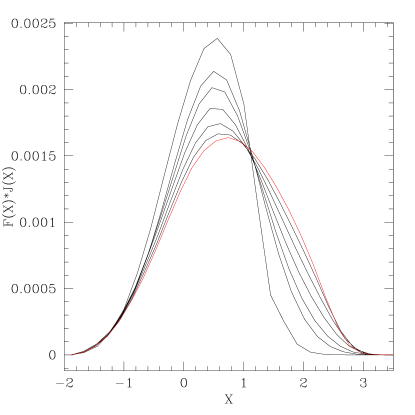
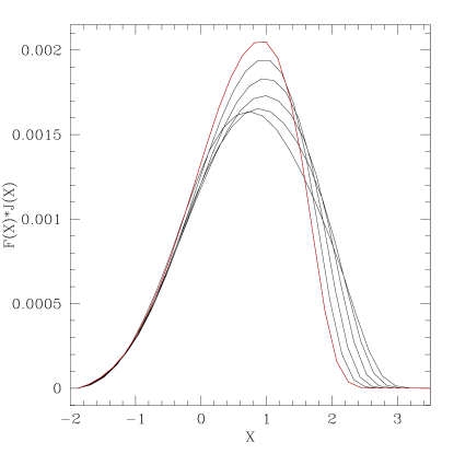
Figure 3 describes the distribution of mass in the mapped energy grid $X$. The quantity $F(X)$ is the phase-space distribution function in the mapped variable $X$ and $J(X)$ describes the phase-space volume between $X$ and $X+dX$. Therefore $F(X)\times J(X)$ is the differential mass. As the potential well evolves, the mapping is rescaled so that inner point has the same value. The first panel in Figure 3 shows the evolution of the mass distribution as it attains the double power law form. For this initial condition, mass is shift outward to populate the higher energy tail. During the second self-similar phase, the double power law profile is established (note the constancy of the profile between $X=-2$ and $X=0$) and further evolution populates the outer tail, driving the $r^{-3}$ profile to larger radii.

(a) King $W_{0}=3$

(b) King $W_{0}=5$

(c) King $W_{0}=7$

(d) Plummer

Figure 2: Evolution of the initial profile (labelled) under ‘shrapnel’ noise. The top curve in each case is the initial profile. The times for each curve are derived using the fiducial scaling from Table 1. The heavy straight lines show power laws with exponent -1.5 and -3.0 for comparison.

(a) Approach to power law profiles

(b) Self-similar phase

Figure 3: For each initial condition (cf. Fig. 2), there are two phases of evolution. In the first phase, the model approaches the double power law profile; the model spreads out in $x$. In the second phase, the double power law slowly evolves; the inner mass distribution evolves self-similarly in $x$ with mass moving outward while the peak at $x\approx 1$ grows. Panels (a) and (b) show the two phases separately. For each of the cases in Fig. 2, the approach phase is completed by 1.0, 0.5, and 0.9 gigayear, respectively.

(a) $m_{sat}/m_{halo}=0.05$

(b) $m_{sat}/m_{halo}=0.03$

(c) $m_{sat}/m_{halo}=0.01$

Figure 4: As in Figure 2) but for noise due to decaying satellite perturbers using the fiducial parameterization from Table 1. Panels (a), (b) and (c) show satellite to halo mass ratios of 0.05, 0.03, and 0.01 respectively.

Figure 5: As in Fig. 2 for a double power law model (eq. 1) with $\gamma=1$, $\beta=4$ and $\epsilon=0.1$.

Figure 6: Evolution of a King $W_{0}=3$ profile under ‘black hole’ noise. The times for each curve are shown with the scaling for number of black holes per halo assuming that the black hole fraction is one ($f_{bh}=1$ in Table 1). Note that for the fiducial number, $n_{bh}=10^{6}$, the evolution time scale is uninterestingly large.

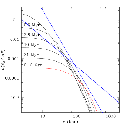
Evolution in the double power model (eq.1) shown in Figure 6 is similar to the cases shown in Figure 2. Beginning with $\gamma=1$, $\beta=4$ and $\epsilon=0.1$, the inner profile quickly attains the same shape as those in Figure 2, with a net transport of mass outward and expansion. The outer profile quickly approaches $r^{-3}$. The evolution is an order of magnitude faster than the cases in Figure 2 with the fiducial parameters given in Table 1 because the dynamical times in the cusp are smaller by the same proportion. Recall that the small time scales in Figure 6 are only consistent with the dynamics if there have be many stochastic events. For example, this better describes a situation with $m_{enc}=0.01$ which increases the times in the figure by 100.

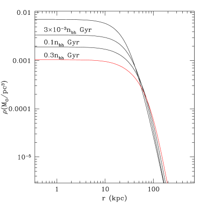
Figure 6 describes the evolution of a $W_{0}=3$ King model due to point mass noise. The evolution rate for this noise source is uninteresting small unless the halo consists of fewer than several hundred holes. Note that because of the small amplitude, curves in the figure are labeled for a single black hole instead of the fiducial scaling given in Table 1. There is little point in characterizing this evolution in any more detail.

5 Discussion

Two of our transient noise sources give double power law profiles: (1) fly-by encounters; and (2) satellite mergers. The evolved halo profiles in each case are quite similar although the trajectories of the perturbers are different. This is explained by the excitation of $l=m=1$ halo mode the low-frequency power in both cases. The sloshing mode results in transport of momentum that gives the shallower inner power-law profile. The response to the external $l=1$ multiple yields the outer $r^{-3}$ profile. The low-frequency power from the decaying satellite comes from the speed of the decay, the changing orbital frequencies in other words, not the orbital frequencies directly. An ensemble of non-decaying satellites drives evolution at harmonics $l>2$ and is relatively weak. For example, a halo of $10^{6}{\rm\,M_{\odot}}$ black holes will cause only minor evolution during the 1 Gyr.

For a initially low-concentration haloes, the inner-profile becomes steeper as it approaches a power law (cf. Fig. 2ab). For high-concentration haloes and all haloes after sufficient time, the core radius slowly increases. This is an artifact of the halo expansion due to the energy added by the noise source. The more centrally concentrated the initial profile, the more rapidly the asymptotic profile obtains. In all cases, the double power law form is evident after several hundred million years for fiducial parameters (see Table 1).

More generally, these results suggest the evolved halo profile will not depend on the noise source in general as long as there is power near the low-order modes. Lowered, truncated isothermal spheres (King models) over an order of magnitude in concentration, $r_{core}/r_{tidal}$, and Plummer spheres all converge to the double power law form. It is difficult to solve the collisional Boltzmann equation (eqs. 2 and A) for initial profiles with large dynamic range owing to numerical limitations. To address initially cuspy profiles, we softened the cusp (cf. eq. 1) and found that the same evolved double power law form obtained and with much smaller time scale because the dynamical times in the cusp are short. For initial conditions without cores, the $l=1$ response will be near the characteristic radius of the initial profile. For example, Weinberg (1998) shows that the $l=1$ mode peaks at the characteristic radius in a Hernquist profile. Moreover, the evolution time scale for a softened cusp model is nearly an order of magnitude shorter under the same noise spectrum as for King models. This further suggests that noise can drive the inner profile of a cuspy dark matter halo to the asymptotic form quite quickly.

These trends may help explain some of the recent trends in cosmological simulations. For isolated haloes, the most massive substructure has decayed or disrupted within 1 Gyr. Figures 2 and 4 show a well-defined inner slope with exponent $\gamma=1.5$ by 1 Gyr. This is consistent with the recent work by Moore et al. (1998) and Klypin et al. (2000). For longer evolution or noisier evolution, the inner exponent continues to evolve, although slowly (cf. Fig. 2). In particular, this may help explain Jing & Suto (2000) finding that the inner slope depends on environment and the evolution of the scale radius $r_{s}$ (e.g. NFW). However, as described in §3, further development needed to address the affect of cuspy initial profiles will be necessary to predict this trend and will be the subject of a later paper.

6 Summary

This paper describes the evolution of a halo due to transient noise typical of the epoch of galaxy formation ($\tau\mathrel{\hbox to0.0pt{\lower 3.0pt\hbox{$\mathchar 536\relax$}\hss}\raise 2.0pt\hbox{$\mathchar 316\relax$}}1{\rm\,Gyr}$). We consider two transient noise sources: fly by encounters and merging substructure (satellites). Both result drive the halo toward double power law profiles with inner exponent of approximately $-1.5$ and outer power law exponent of $-3$, similar to the form proposed by NFW and Moore et al. Over a range of initial halo concentrations, the double power laws obtain independent of noise source and initial profile.

The dynamical mechanism is simply explained. When one disturbs a halo it rings. This ringing is damped but the mostly weakly damped modes shape the response and dominate the angular momentum transport responsible for evolution. Therefore, it doesn’t matter how one hits the halo, as long as the modes can be excited, the evolution looks the same. The dominant modes are low frequency and low harmonic order (dipoles) and can be driven by a wide variety of transient noise sources. The outer power law exponent, $-3$, is due to the repetitive excitation and response of the halo to the outer $l=1$ multipole. The common appearance of the $r^{-3}$ profile in n-body simulations suggests a noise-driven origin.

This noise driven evolution provides a natural explanation for the near universality of the halo profiles found in CDM simulations and may provide an explanation for a spread of inner power law exponents. Variation in the substructure at different scales (either due to the CDM power spectrum or dynamic range of the simulation) and differences in the initial halo profile will produce different exponents at the same point in time. Additional work will be required to make precise predictions for these trends. Nonetheless, this work shows that noise naturally drives halo evolution with near-universal form.

Appendix A Fokker-Planck evolution equation

From the development in Paper 1, we have that equation describing the evolution under noise processes is:

$${\partial f^{\prime}({\bf I},t)\over\partial t}=\left[-{\partial\over\partial I_{k}^{\prime}}D_{k}^{\prime}+{\partial^{2}\over\partial I_{k}^{\prime}\partial I_{l}^{\prime}}D_{kl}^{\prime}\right]f^{\prime}({\bf I},t),$$ (2)

where the $D_{k}$ and $D_{kl}$ are the time derivative of the action moments due to the noise process. The isotropically averaged Fokker-Planck becomes

$${\partial f(E)\over\partial\,t} = {1\over P(E)}{\partial\over\partial E}\left[-\langle D_{E}\rangle_{iso}P(E)f(E)\right.$$

$$+\left.{\partial\over\partial E}\left(\langle D_{EE}\rangle_{iso}P(E)f(E)\right)\right]$$

where $P(E)$ is the phase space volume between $E$ and $E+dE$. The moment coefficients $D_{E}$ and $D_{EE}$ can not be strictly interpreted as advection and diffusion. In particular the first-moment term may be positive or negative at different energies depending on the structure of the response and its frequency spectrum.

Appendix B Numerical implementation

We solve the evolution equation (A) using a two-step splitting technique following the work on globular cluster evolution. First, the gravitational potential is held fixed and the phase-space distribution function is evolved. The Fokker-Planck equation is finite-differenced in energy using the Crank-Nicholson scheme in flux-conserving form. Because the “advection” term can be both positive and negative, the Chang-Cooper algorithm does not apply (Chang & Cooper 1970). The energy variable is remapped as described in Appendix C to improve the dynamic range. After exploring a number of possibilities, the range of the energy grid extends from the centre to $E\rightarrow 0$. The boundary conditions, then, are zero flux through the boundary. In practice, the outer boundary is set to $E=-\epsilon$ for some small $\epsilon$ which corresponds to some large radius. Second, the potential and density distribution with new distribution is solved iteratively to convergence. To do this, the distribution of actions is held fixed and a self-consistent spatial profile is determined by computing a new density distribution from the phase-space distribution function and the current gravitational potential. One then computes a new gravitational potential from the new density profile and continues. We construct the mapping between energy $E$ and angular momentum $J$ and the radial actions by using the marching squares algorithm on a two-dimensional table of radial action as a function $E$, and angular momentum $J/J_{max}(E)$. The profile recomputed when central density has changed by 2%. Empirically, 40 or 100 mesh points in the transformed energy grid are sufficient for low and high concentration models, respectively.

The moment coefficients $D_{E}$ and $D_{EE}$ defined in Paper 1 are expensive and recomputed only when central density has changed by 5%. The discrete sums in the action-angle series are typically truncated at $l_{1\,max}=10$. For low-order expansions here, $l\leq 4$, this is sufficient to include at least 95% of the total contribution. We use the biorthogonal basis described Weinberg (1999) and truncate the expansion at $n_{max}=10$. This basis uses direct solution of the Sturm-Liouville equation to find a basis whose lowest order function matches the equilibrium profile. The results were checked in several cases using both the Clutton-Brock (1973) and Hernquist & Ostriker (1992) bases along with tests of varying $l_{1\,max}$, $n_{max}$ and energy grids with comparable results. The asymptotic double power law form reported here shows no signs of being a numerical artifact.

Appendix C Energy grid mapping

In order to to resolve the distribution function over a large dynamic range, one can remap the energy to distribute mesh points more uniformly between the cusp and outer profile. The following mapping as proved useful in globular cluster work (Chernoff & Weinberg 1990) and we will adopt it here.

$$x=-\log\left({E\over(2-\alpha)E_{0}-E}\right)$$ (4)

where $E_{0}$ is the smallest (most bound) energy and $\alpha$ is a fixed parameter. For small values of $\alpha$, this transformation is becomes purely logarithmic. As $\alpha\rightarrow 1$ the mapping diverges as $E\rightarrow E_{0}$. By carefully choosing values $\alpha<1$, we can place more grid points in the centre to better resolve the profile. For these calculations, $\alpha=0.85$ is a good choice.

Changing variables as described in Paper 1 yields:

$$D_{x}={\partial x(E)\over\partial I_{j}}D_{j}+{\partial^{2}x(E)\over\partial I_{i}\partial I_{j}}D_{ij}.$$ (5)

where

$${\partial x(E)\over\partial I_{j}} = {dx(E)\over dE}\Omega_{j}$$ (6)

$${\partial^{2}x(E)\over\partial I_{i}\partial I_{j}} = {dx(E)\over dE}{\partial\Omega_{j}\over\partial I_{i}}+{d^{2}x(E)\over dE^{2}}\Omega_{i}\Omega_{j}.$$ (7)

Altogether we have:

$$D_{x} = {dx(E)\over dE}\Omega_{j}D_{j}+{dx(E)\over dE}{\partial\Omega_{j}\over\partial I_{i}}D_{ij}+{d^{2}x(E)\over dE^{2}}\Omega_{i}\Omega_{j}D_{ij}$$

$$D_{xx} = \left({dx(E)\over dE}\right)^{2}\Omega_{i}\Omega_{j}D_{ij}$$ (9)

In this mapped energy variable, the Fokker Planck equation (cf. eq. A) becomes

$${\partial f(E(x))\over\partial\,t} = {1\over P(E(x))J_{x}(x)}\times$$

$${\partial\over\partial x}\left[\rule{0.0pt}{15.0pt}-D_{x}P(E(x))J_{x}f(E(x))\right.$$

$$+\left.{1\over J_{x}(x)}{\partial\over\partial x}\left(D_{xx}P(E(x))J_{x}f(E(x))\right)\right]$$

where

$$J_{x}(x)\equiv{dE\over dx}=-{(2-\alpha)E_{0}e^{-x}\over(1+e^{-x})^{2}}.$$ (11)

References

- [] Alvares, M., Shapiro, P. R., and Martel, H. 2000, The Effect of Gasdynamics on the Structure of Dark Matter Halos, astro-ph/0006203.
- [] Binney, J. and Tremaine, S. 1987, Galactic Dynamics, Princeton University Press, Princeton, New Jersey.
- [] Chang, J. S. and Cooper, G. 1970, J. Comp. Phys., 6, 1.
- [] Chernoff, D. F. and Weinberg, M. D. 1990, ApJ, 351, 121.
- [] Clutton-Brock, M. 1973, Astrophys. Space. Sci., 23, 55.
- [] Frenk, C. S., White, S. D. M., Bode, P., Bond, J. R., Bryan, G. L., Cen, R., Couchman, H. M. P., Evrard, A. E., Gnedin, N., Jenkins, A., Khokhlov, A. M., Klypin, A., Navarro, J. F., Norman, M. L., Ostriker, J. P., Owen, J. M., Pearce, F. R., Pen, U. ., Steinmetz, M., Thomas, P. A., Villumsen, J. V., Wadsley, J. W., Warren, M. S., Xu, G., and Yepes, G. 1999, ApJ, 525, 554.
- [] Hernquist, L. and Ostriker, J. P. 1992, ApJ, 386, 375.
- [] Jing, Y. P. and Suto, Y. 2000, ApJL, 529, L69.
- [] King, I. R. 1966, AJ, 71, 64.
- [] Klypin, A., Kravtsov, A. V., Bullock, J., and Primack, J. 2000, in submitted to ApJ, 16 pages, 10 figures, uses aastex and natbib., pp 6343.
- [] Lacey, C. G. and Ostriker, J. P. 1985, ApJ, 299, 633.
- [] Moore, B., Ghigna, S., Governato, F., Lake, G., Quinn, T., Stadel, J., and Tozzi, P. 1999, ApJL, 524, L19.
- [] Moore, B., Governato, F., Quinn, T., Stadel, J., and Lake, G. 1998, ApJL, 499, L5.
- [] Navarro, J. F., Frenk, C. S., and White, S. D. M. 1997, ApJ, 490, 493.
- [] Spergel, D. N. and Steinhardt, P. J. 2000, Phys. Rev. Lett., 84, 3760.
- [] Tittley, E. R. and Couchman, H. M. P. 1999, Hierarchical clustering, the universal density profile, and the mass-temperature scaling law of galaxy clusters, astro-ph/9911365.
- [] Tormen, G., Diaferio, A., and Syer, D. 1998, MNRAS, 299, 728.
- [] Vesperini, E. and Weinberg, M. D. 2000, ApJ, 534, 598.
- [] Weinberg, M. D. 1998, MNRAS, 299, 499.
- [] Weinberg, M. D. 1999, AJ, 117, 629.
- [] Weinberg, M. D. 2000, MNRAS, submitted (Paper 1).