Mapping the star formation history of Mrk~86^∗

Abstract

In this paper, continuation of Gil de Paz et al. (Paper I), we derive the main properties of the stellar populations in the Blue Compact Dwarf galaxy Mrk~86. Ages, stellar masses, metallicites and burst strengths have been obtained using the combination of Monte Carlo simulations, a maximum likelihood estimator and Cluster and Principal Component Analysis. The three stellar populations detected show well defined properties. We have studied the underlying stellar population, which shows an age between 5-13 Gyr and no significant color gradients. The intermediate aged (30 Myr old) central starburst show a very low dust extinction with high burst strength and high stellar mass content ($\sim$9$\times$10⁶ M_☉). Finally, the properties of 46 low-metallicity ($\sim$1/10 Z_☉) star-forming regions were also studied.

The properties derived suggest that the most recent star-forming activity in Mrk~86 was triggered by the evolution of a superbubble originated at the central starburst by the energy deposition of stellar winds and supernova explosions. This superbubble produced the blowout of a fraction of the interstellar medium at distances of about 1 kpc with high gas surface densities, leading to the activation of the star formation.

Finally, different mechanisms for the star formation triggering in this massive central starburst are studied, including the merging with a low mass companion and the interaction with UGC~4278. We have assumed a distance to Mrk~86 of 6.9 Mpc.

1 Introduction

The high star formation rate (SFR hereafter) and low neutral gas content deduced for dwarf star-forming galaxies imply consumption time-scales of about 10⁹ yr (Fanelli et al. fanelli (1988); Thuan & Martin thuan81 (1981)), much shorter than the age of the Universe. Searle et al. (searle73 (1973)) suggested that either these objects are truly young systems or they have an intermittent star formation history with short intense star-forming episodes followed by long quiescent phases. Although this question remained unanswered during decades (Thuan thuan83 (1983); Campbell & Terlevich campbell (1984); Loose & Thuan loose85 (1985)), nowadays, most of the studies on dwarf star-forming systems, including Blue Compact Dwarf galaxies (BCD hereafter), have revealed the existence of an evolved underlying population (Kunth et al. kunth88 (1988); Hoffman et al. hoffman (1990); Papaderos et al. 1996b ; Doublier doublier98 (1998); Norton & Salzer norton (1997)).

Therefore, the understanding of the mechanism, or mechanisms, governing this star formation regulation is the stepping stone of the dwarf star-forming galaxies evolution. Moreover, this mechanism constitutes the missing link between the different dwarf star-forming galaxies (Silk et al. silk87 (1987); Burkert burkert (1989); Drinkwater & Hardy drinkwater (1991); Papaderos et al. 1996b ).

There are two different approaches to address these questions. On the one hand, statistical analysis of a sample of these objects will allow the study of the relationships between fundamental parameters and properties of the star-forming dwarf galaxies (Marlowe et al. marlowe95 (1995); Papaderos et al. 1996a , 1996b ). On the other hand, the detailed analysis of individual low-redshift objects with multiple regions of star formation is fundamental to reconstruct their star formation histories. In particular, we can obtain a better understanding of possible effects of merging or some internal process as self-propagation that could originate the spreading of star formation, and the effects of these star-forming events on the future star formation.

Among dwarf galaxies, Blue Compact Dwarf galaxies conform the subpopulation where the star-forming events are most violent. Blue Compact Dwarfs are low-luminosity (M_B $\geq$$-$18^m) galaxies with compact sizes whose spectra are similar to those of low metallicity H ii regions (Searle & Sargent searle72 (1972); Kunth & Sargent kunth86 (1986); Thuan & Martin thuan81 (1981)). Their spectra are characterized by emission lines over a blue continuum which implies the existence of a large fraction of OB stars and an intense star-forming activity.

The Blue Compact Galaxy Mrk~86=NGC~2537 (Shapley & Ames shapley32 (1932); Markarian markarian69 (1969)), also known as Arp 6 (Arp arp66 (1966)), constitutes an excellent laboratory to test the BCD star formation history since its star-forming regions populate all the galaxy. This object is the propotype of the iE galaxies, the most important BCD galaxies subclass, that conform 70 per cent of the BCD galaxies (Thuan & Martin thuan81 (1981); Thuan thuan91 (1991)).

In Gil de Paz et al. (2000a ; Paper I hereafter) we presented observational data for the underlying population and star-forming regions of Mrk~86. We provided sizes, $BVRJHK$ magnitudes, colors and emission-line fluxes for most of these regions. The evolutionary synthesis models used in this paper were also extensively described.

Now, we describe the procedure employed to compare the colors measured and those predicted by the evolutionary synthesis models in Sect. 2. The properties of the underlying stellar population, central starburst and recent star-forming regions are studied in Sect. 3.1,  3.2 and 3.3, respectively. Electron densities, temperatures and metal abundances for the brightest star-forming regions in the galaxy are given in Sect. 3.4. Finally, in Sect. 4, we provide a global interpretation of the short- and mid-term star formation history of the galaxy. The main conclusions from this study are summarized in Sect. 5.

2 Data-models comparison method

2.1 Determination of the underlying population properties

The optical-near-infrared colors measured for the underlying stellar component (see Sect. 5 and 6.1 in Paper I) have been compared with those predicted by the Bruzual & Charlot (priv. comm.) evolutionary synthesis models. We have obtained the best-fitting model for each point in the color profiles (see Fig. 6 of Paper I) using a maximum likelihood estimator. This maximum likelihood estimator is defined as,

$${\cal L}(t,b,Z)=\prod_{n=1}^{5}{1\over\sqrt{2\pi}\Delta C_{n}}\exp\left(-{(c_{n}-C_{n})^{2}\over 2\Delta C_{n}\,^{2}}\right)$$ (1)

where $C_{n}$ (with $n$=1-5) are the $B-V$, $V-R$, $R-J$, $J-H$ and $R-K$ colors measured, and $c_{n}$ are those predicted by the evolutionary synthesis models. The colors measured were corrected for Galactic extinction using an extinction in the $B$-band of 0.15^m (Burstein & Heiles burstein (1982)).

We have studied different star formation histories for the formation of this component. In particular, we have considered instantaneous and 1, 3 and 7 Gyr duration bursts and continuous star formation models. This comparison has been restricted to models with metallicity lower than the solar value. We are confident with this assumption since the gas metallicities derived in Sect. 3.4 for the galaxy star-forming regions are lower than one tenth solar.

2.2 Determination of the star-forming regions properties

A more elaborated comparison method has been used in the case of the galaxy star-forming regions. This comparison method is fully described in Gil de Paz et al. (2000b ). Briefly, it combines Monte Carlo simulations and a maximum likelihood estimator with Cluster and Principal Component Analysis.

The maximum likelihood estimator employed is very similar to that described in Sect. 2.1, but replacing the $R-J$ and $R-K$ colors by the $V-J$ and $J-K$ colors. In addition, since these regions have intense H$\alpha$ emission, we have included a new term, defined as $m_{R}$+2.5$\times$log($F_{\mathrm{H}\alpha}$). This term is equivalent to the H$\alpha$ equivalent width (EW hereafter) term, 2.5$\times$log EW(H$\alpha$), used in Gil de Paz et al. (2000b ). The $m_{R}$ magnitudes are those measured within the apertures given in Paper I.

Table 1: Age and mass-to-light ratio for the underlying stellar population. The best-fitting model in all these solutions is two-fifths solar metal abundant. Solutions for an instantaneous, 1, 3 and 7 Gyr duration burst and constant star formation rate models are shown.

	$A_{B,\mathrm{i}}$†=0.0m		$A_{B,\mathrm{i}}$=0.20m		$A_{B,\mathrm{i}}$=0.0m		$A_{B,\mathrm{i}}$=0.20m		$A_{B,\mathrm{i}}$=0.0m		$A_{B,\mathrm{i}}$=0.20m
$d$	$t$	$M/L_{K}$‡	$t$	$M/L_{K}$	$t$	$M/L_{K}$	$t$	$M/L_{K}$	$t$	$M/L_{K}$	$t$	$M/L_{K}$
(kpc)	(Gyr)		(Gyr)		(Gyr)		(Gyr)		(Gyr)		(Gyr)
	Instantaneous burst				1 Gyr burst				3 Gyr burst
0.88	5.0	0.62	2.2	0.41	5.5	0.62	3.0	0.44	6.5	0.62	4.0	0.43
0.97	5.2	0.63	2.4	0.44	6.0	0.64	3.2	0.46	7.2	0.67	4.2	0.45
1.06	6.0	0.68	3.8	0.56	6.5	0.68	3.8	0.48	8.5	0.74	5.0	0.51
1.16	8.7	0.83	5.2	0.63	9.8	0.86	5.8	0.63	10.5	0.85	6.5	0.62
1.27	8.0	0.80	3.8	0.56	8.5	0.80	5.2	0.61	9.2	0.79	5.8	0.56
1.36	9.5	0.87	5.5	0.64	9.8	0.86	6.0	0.64	11.2	0.88	7.2	0.67
1.47	9.5	0.87	5.8	0.66	9.8	0.86	6.2	0.66	11.2	0.88	7.2	0.67
1.57	9.5	0.87	5.5	0.64	9.8	0.86	6.0	0.64	11.2	0.88	7.2	0.67

	$A_{B,\mathrm{i}}$=0.0m		$A_{B,\mathrm{i}}$=0.20m		$A_{B,\mathrm{i}}$=0.0m		$A_{B,\mathrm{i}}$=0.20m
$d$	$t$	$M/L_{K}$	$t$	$M/L_{K}$	$t$	$M/L_{K}$	$t$	$M/L_{K}$
(kpc)	(Gyr)		(Gyr)		(Gyr)		(Gyr)
	7 Gyr burst				Continuous
0.88	8.5	0.58	7.2	0.49	$>$20	$>$0.73	19.2	0.72
0.97	9.2	0.64	7.5	0.51	$>$20	$>$0.73	$>$20	$>$0.73
1.06	10.8	0.74	7.8	0.53	$>$20	$>$0.73	$>$20	$>$0.73
1.16	12.2	0.82	9.0	0.62	$>$20	$>$0.73	20.0	0.73
1.27	11.2	0.76	7.8	0.53	$>$20	$>$0.73	$>$20	$>$0.73
1.36	13.0	0.86	9.2	0.64	$>$20	$>$0.73	20.0	0.73
1.47	13.8	0.90	9.8	0.67	$>$20	$>$0.73	20.0	0.73
1.57	13.0	0.86	9.2	0.64	$>$20	$>$0.73	20.0	0.73

^† $A_{B,\mathrm{i}}\equiv A_{B,\mathrm{internal}}$
^‡ $M/L_{K}$ is expressed in M_☉/L_K,☉

In order to properly derive this new term, we have computed the fraction of H$\alpha$ flux, i.e. the fraction of Lyman photons, due to the stellar continuum measured within the apertures. Two different approaches can be followed. First, we could measure the H$\alpha$ fluxes using these apertures. However, since the H$\alpha$ emission is usually more extended than the continuum emisson, this procedure would sistematically underestimate the H$\alpha$ flux (see, e.g. #8, #13, #18, #50, #70 and #80 regions). Therefore, we have used an alternative method. We measured the total H$\alpha$ using the cobra program (see Paper I). Then, we assumed that the fraction of photons emitted within the apertures relative to the total emission is equivalent for the Lyman and $R$-band continuum. Thus, considering that the apertures were obtained at e-, e²- or e³-folding radii and assuming gaussian ligth profiles, this light fraction can be computed for each region. The values obtained for this fraction, $f$, are given in Table 3.

Then, multiplying these flux ratios by the total H$\alpha$ fluxes given in Table 4 of Paper I, we derive the H$\alpha$ luminosities due to the continuum emission measured within the apertures.

The H$\alpha$ fluxes were corrected for extinction using the $E(B-V)_{\mathrm{gas}}$ color excesses provided by the H$\beta$-H$\alpha$, H$\gamma$-H$\beta$ Balmer decrements. In addition, the broad-band magnitudes and colors were corrected for extinction assuming that the extinction affecting the stellar continuum and the gas extinction are related via $E(B-V)_{\mathrm{continuum}}$=0.44$\times$$E(B-V)_{\mathrm{gas}}$ (Calzetti et al. calzetti (1996)). In those regions where Balmer line ratios were not measurable we assumed an average extinction of $E(B-V)_{\mathrm{gas}}$=0.34^m. This value was obtained as the mean of the color excesses given in Table 5 of Paper I for those regions with accessible Balmer line ratios.

Thus, each star-forming region has a point associated in the $B-V$, $V-R$, $V-J$, $J-H$, $J-K$, $m_{R}$$+$2.5$\times$log($F_{\mathrm{H}\alpha}$) six-dimensional space. However, the corresponding uncertainties transform these points into probability distributions. Using a Monte Carlo method with 10³ points and assuming gaussian errors we reconstructed these probability distributions. Then, we compared each of these 10³ points with our models using the maximuum likelihood estimator described above. Since these models are parametrized in age, $t$; burst strength, $b$; and metallicity, $Z$, of the burst stellar population, this method effectively provides the ($t$,$b$,$Z$) probability distribution for each input region (see Table 3).

Finally, we studied the clustering pattern present in these distributions using a hierarchical clustering method (see Murtagh & Heck murtagh (1987)). This method allows to isolate different solutions in the ($t$,$b$,$Z$) space. We grouped the 10³ ($t$,$b$,$Z$) points in three clusters of solutions. Then, we performed a Principal Component Analysis (see Morrison morrison (1976)) for each individual solution (see Gil de Paz et al. 2000b for a more complete description of this procedure).

For the central starburst component we used a similar procedure. However, since no H$\alpha$ emission was detected for this component, the $m_{R}$$+$2.5$\times$log($F_{\mathrm{H}\alpha}$) term was not included in the maximum likelihood estimator. In addition, we introduced the continuum color excess $E(B-V)$ as a free parameter. Color excesses in the range 0.0-1.0^m were studied, where 0.05^m is the Galactic color excess. For each of the 10³ Monte Carlo particles the full range was explored, obtaining the best-fitting color excess and ($t$,$b$,$Z$) array.

3 Results

3.1 Underlying population

In this section we describe the results obtained after comparing the colors measured and those predicted by the evolutionary synthesis models.

We compared the model predictions with the optical-near-infrared colors measured without correcting for internal extinction ($A_{B,\mathrm{internal}}$=0.0^m) and using an extinction correction factor of 0.20^m in the $B$-band. The latter value corresponds approximately to two times the extinction of a Galactic-type disk with an inclination of 40^∘ relative to the plane of the sky (see Gil de Paz et al. GZG (1999), GZG hereafter; see also Gil de Paz gilphd (2000)). Therefore, the results obtained applying these extinction correction factors can be taken as upper and lower limits for the age and mass-to-light ratio of this population, respectively.

The same metallicity, 2/5 Z_☉, was obtained at any galactocentric distance in the interval 0.9-1.6 kpc. Since these results, basically age and mass-to-light ratio, were obtained using only aperture colors, they are not affected by the distance uncertainty described in Sect. 2.1 of Paper I.

The ages derived range between 5.0 Gyr at galactocentric distances of about 0.9 kpc and 9.5 Gyr at distances larger than 1.3 kpc (for an instantaneous burst and $A_{B,\mathrm{internal}}$=0.0^m). The corresponding interval in $K$-band mass-to-light ratio was 0.62-0.87 M_☉/L_K,☉ (see Table 1). The change in the age and mass-to-light ratio of the stellar population at distances shorter than 1.3 kpc is due to contamination from the plateau component (see the $B$-band profile decomposition given in Papaderos et al. 1996a ). Since the spatial extent of this component coincides with the H$\alpha$ emitting zone (see Fig. 7 in Paper I), this contamination is probably related with a progressively higher contribution of the recent star-forming regions to the total emission.

The outer region of the galaxy color profiles seems to indicate that no significant age gradients are present. However, a small positive metallicity or extinction gradient could compensate the existence of a negative age gradient, or vice versa, reproducing the observed color profiles.

The results shown in Table 1 also suggest that, although the age of the underlying stellar population ($d$$>$1.3 kpc) could range between 5 and 13 Gyr depending on the star formation history considered, the mass-to-light ratio in the $K$-band is very well constrained for a given extinction correction. Thus, the $K$-band mass-to-light ratio for $A_{B,\mathrm{internal}}$=0.0^m is approximately 0.87 $M_{\sun}/L_{K,\sun}$ and 0.65 $M_{\sun}/L_{K,\sun}$ for $A_{B,\mathrm{internal}}$=0.20^m.

The small differences ($<$30 per cent) obtained in the maximuum likelihood estimator after comparing our data with models with burst duration shorter than 7 Gyr prevent us to infer the star formation history and internal extinction of the underlying stellar population. Therefore, we are not able to determine if this stellar population has effectively formed in a instantaneous burst or during long (several Gyr) periods of time as it has been observed in I~Zw~18 (Aloisi et al. aloisi99 (1999)). Only continuous star formation models (or with a duration for the burst longer than 7 Gyr) can be rule out since their very low maximuum likelihood estimators and too old ages derived.

The evolutionary synthesis models developed for the analysis of the star-forming regions properties only depend on the observed colors and mass-to-light ratio of the underlying stellar population. Therefore, the conclusions given in Sect. 3.3 for the study of these regions are not affected by our ignorance on the past star formation history of the galaxy.

In order to build these models (see Paper I and Sect. 3.3) we adopted a mass-to-light ratio for the underlying stellar population of 0.87 M_☉/L_K,☉ in the $K$-band, which corresponds to a null internal extinction value. However, if the internal extinction was relatively higher, e.g. $A_{B,\mathrm{internal}}$=0.20^m, the mass-to-light ratio could be a 25 per cent lower yielding slightly different properties for the most recent star-forming regions (see Sect. 3.3).

3.2 Central starburst

After applying the comparison procedure described in Sect. 2.2, we obtained the three clusters of solutions in the age, burst strength, metallicity and color excess four-dimensional space. Two of these three solutions show probabilites lower than 1 per cent. In Fig. 1 we show the distribution of the total number of solutions obtained within the remaining solution cluster which has a probability of 98 per cent.

Figure 1: Frequency histograms for the central starburst a) age, b) burst strength, c) continuum color excess and d) stellar mass.

The age obtained for the starburst component is about 30 Myr, and the burst strength is 20 per cent. Fig. 1c shows that the continuum color excess is very well constrained between 0.06 and 0.08^m. The starburst age derived agrees with the absence of H$\alpha$ emission for this component. The expected H$\alpha$ equivalent width in emission at ages older than 30 Myr and 20 per cent burst strength is lower than 2 Å for any stellar metallicity.

Table 2: Spectroscopic indexes for the underlying population (2/5 Z_☉ metal abundant), starburst component (2/5 Z_☉ and 1/5 Z_☉ metal abundant) and for the composite stellar population using a 30 Myr old burst with burst strengths 20, 10 and 5 per cent. EW(H$\delta$) and Fe5270 and Fe5406 indexes are expressed in Å.

Starburst metallicity: Z=2/5 Z☉
	Under.	Starb.	Composed	Obs.	Cor.
			b=0.2/0.1/0.05
Mg2	0.186	0.042	0.05/0.07/0.08	0.06	0.08
EWHδ	2.91	6.18	5.89/5.59/5.14	6.0
D4000	2.01	1.14	1.19/1.24/1.32	1.38	1.38
Fe5270	2.508	0.625	0.95/1.23/1.57	1.20	1.10
Fe5406	1.369	0.371	0.54/0.69/0.87	0.74	0.66
Starburst metallicity: Z=1/5 Z☉
	Under.	Starb.	Composed	Obs.	Cor.
			b=0.2/0.1/0.05
Mg2	0.186	0.035	0.05/0.06/0.08	0.06	0.08
EWHδ	2.91	6.43	6.11/5.78/5.30	6.0
D4000	2.01	1.16	1.21/1.26/1.34	1.38	1.38
Fe5270	2.508	0.723	1.03/1.29/1.60	1.20	1.10
Fe5406	1.369	0.374	0.54/0.69/0.86	0.74	0.66

In order to confirm these results, we will compare the H$\delta$ equivalent width and D₄₀₀₀, Mg2, Fe5270 and Fe5406 spectroscopic indexes measured with the values predicted by the evolutionary synthesis models. Unfortunately, we only dispose of spectroscopic index predictions for the case of pure burst models. Therefore, we will derive the spectroscopic indexes of this component using the predictions from pure burst models and the burst strength given above. In this way, a molecular index like Mg2 (see Gorgas et al. gorgas93 (1993)), can be written for a composite stellar population as

$$\mathrm{Mg2}=\mathrm{Mg2}_{\mathrm{s}}-2.5\log\frac{1+\frac{1-b}{b}\frac{MLR_{\mathrm{s}}}{MLR_{\mathrm{u}}}10^{-0.4(\mathrm{Mg2}_{\mathrm{u}}-\mathrm{Mg2}_{\mathrm{s}})}}{1+\frac{1-b}{b}\frac{MLR_{\mathrm{s}}}{MLR_{\mathrm{u}}}}$$ (2)

where, Mg2_u and Mg2_s are the spectroscopic indexes for the underlying stellar population and the young starburst, $MLR_{\mathrm{u}}$ and $MLR_{\mathrm{s}}$ are the mass-to-ligth ratios at the continuum and $b$ is the burst strength in mass. The mass-to-ligth ratios $MLR_{\mathrm{u}}$ and $MLR_{\mathrm{s}}$ are, respectively, 3.436 and 0.084 M_☉/L_B,☉ in the $B$-band (Bruzual & Charlot priv. comm. for Z=2/5 Z_☉), using $M_{B,\sun}$=5.51 (Worthey worthey (1994)). In the case of an atomic index (Fe5270 and Fe5406) or the equivalent width of H$\delta$, it can be derived using

$$\mathrm{EW(H}\delta\mathrm{)}=\frac{(1-b)MLR_{\mathrm{s}}\mathrm{EW(H}\delta\mathrm{)}_{\mathrm{u}}+b\ MLR_{\mathrm{u}}\mathrm{EW(H}\delta\mathrm{)}_{\mathrm{s}}}{(1-b)MLR_{\mathrm{s}}+b\ MLR_{\mathrm{u}}}$$ (3)

where EW(H$\delta$)_u and EW(H$\delta$)_s are the H$\delta$ equivalent widths (or Fe5270 and Fe5406 indexes) of the underlying and young stellar populations.

Finally, we define the D₄₀₀₀ index (Bruzual bruzual (1983); Gorgas et al. gorgas (1999)) as

$$\mathrm{D}_{4000}=\frac{\int_{4250(1+z)}^{4050(1+z)}\lambda^{2}f_{\lambda}d\lambda}{\int_{3750(1+z)}^{3950(1+z)}\lambda^{2}f_{\lambda}d\lambda}$$ (4)

Then, assuming

$$\frac{\int_{4250(1+z)}^{4050(1+z)}\lambda^{2}f_{\lambda,\mathrm{u}}d\lambda}{\int_{4250(1+z)}^{4050(1+z)}\lambda^{2}f_{\lambda,\mathrm{s}}d\lambda}=\frac{1-b}{b}\frac{MLR_{\mathrm{s}}}{MLR_{\mathrm{u}}}$$ (5)

where $f_{\lambda,\mathrm{u}}$ and $f_{\lambda,\mathrm{s}}$ are the fluxes per unit wavelength of the underlying and starburst populations ($f_{\lambda}$=$f_{\lambda,\mathrm{u}}$$+$$f_{\lambda,\mathrm{s}}$), we obtain the following expression for the D₄₀₀₀ index,

$$\mathrm{D}_{4000}=\frac{(1-b)MLR_{\mathrm{s}}+b\ MLR_{\mathrm{u}}}{(1-b)MLR_{\mathrm{s}}(\frac{1}{\mathrm{D}_{4000,\mathrm{u}}})+b\ MLR_{\mathrm{u}}(\frac{1}{\mathrm{D}_{4000,\mathrm{s}}})}$$ (6)

The continuum mass-to-ligth ratios used were those predicted for the $B$-band in the Mg2, EW(H$\delta$) and D₄₀₀₀ cases and for the $V$-band in the case of the iron indexes ($MLR_{\mathrm{u},V}$=2.80 M_☉/L_V,☉ and $MLR_{\mathrm{s},V}$=0.0147 M_☉/L_V,☉ for Z=2/5 Z_☉). The latter mass-to-light ratios were obtained using $M_{V,\sun}$=4.84 (Worthey worthey (1994)).

Figure 2: Frequency histograms for the age (upper panels), burst strength (central panels) and stellar mass (lower panels) of the star-forming regions. These distributions have been obtained considering only one solution for each star-forming region. This solution corresponds to the mean of the highest-probability solution cluster. (see Table 3)

Table 3: Mean value and standard deviation for the age, burst strength, mass and metallicity of each individual cluster of solutions. Only the properties of those clusters with probability higher than 20 per cent for each region in column 1 are given. Results for models with 15 per cent and a null fraction of Ly photons escaping from the galaxy are shown separately. Probabilities for these clusters of solutions are given in columns 6 and 11. Metallicity is expressed as log($Z$/$Z_{\sun}$).

Any metallicity
	15% escaping Ly photons					0% escaping Ly photons
#	Age	log $b$	$Z$	log $M$	Probab.	Age	log $b$	$Z$	log $M$	Probab.	$f$
	(Myr)			(M☉)	(%)	(Myr)			(M☉)	(%)	(%)
6	6.03$\pm$0.73	$-$2.02$\pm$0.34	$-$0.45$\pm$0.11	3.76$\pm$0.35	94.9	6.00$\pm$0.75	$-$2.03$\pm$0.35	$-$0.45$\pm$0.12	3.75$\pm$0.35	94.6	72.0
7	6.76$\pm$1.06	$-$2.14$\pm$0.34	0.31$\pm$0.17	3.94$\pm$0.35	76.7	6.75$\pm$1.05	$-$2.14$\pm$0.34	0.31$\pm$0.16	3.94$\pm$0.35	76.5	64.2
7	6.98$\pm$0.69	$-$2.47$\pm$0.22	$-$0.41$\pm$0.06	3.72$\pm$0.22	22.7	6.98$\pm$0.68	$-$2.47$\pm$0.22	$-$0.41$\pm$0.06	3.72$\pm$0.22	22.9
8	5.57$\pm$0.43	$-$1.75$\pm$0.17	0.40$\pm$0.02	4.19$\pm$0.18	82.9	5.57$\pm$0.44	$-$1.75$\pm$0.17	0.40$\pm$0.02	4.18$\pm$0.19	82.8	69.2
12	6.75$\pm$0.92	$-$2.12$\pm$0.31	0.33$\pm$0.15	3.91$\pm$0.32	76.2	6.75$\pm$0.93	$-$2.13$\pm$0.31	0.33$\pm$0.15	3.91$\pm$0.32	75.9	71.9
12	7.53$\pm$1.48	$-$2.40$\pm$0.32	$-$0.44$\pm$0.10	3.75$\pm$0.32	20.5	7.53$\pm$1.48	$-$2.41$\pm$0.34	$-$0.45$\pm$0.11	3.73$\pm$0.35	20.8
13	5.00$\pm$0.13	$-$1.52$\pm$0.16	0.40	4.93$\pm$0.19	52.1	5.01$\pm$0.13	$-$1.51$\pm$0.17	0.40	4.92$\pm$0.20	53.6	51.6
13	6.36$\pm$0.17	$-$1.68$\pm$0.07	$-$0.40$\pm$0.01	4.93$\pm$0.07	47.4	6.35$\pm$0.18	$-$1.68$\pm$0.07	$-$0.40$\pm$0.01	4.93$\pm$0.07	46.0
14	7.01$\pm$1.11	$-$1.70$\pm$0.47	0.28$\pm$0.18	4.20$\pm$0.50	60.6	7.00$\pm$1.11	$-$1.71$\pm$0.47	0.29$\pm$0.18	4.19$\pm$0.50	60.7	77.3
14	7.64$\pm$0.68	$-$2.02$\pm$0.17	$-$0.41$\pm$0.06	4.12$\pm$0.17	39.2	7.63$\pm$0.67	$-$2.02$\pm$0.17	$-$0.41$\pm$0.06	4.12$\pm$0.17	39.1
15	8.80$\pm$0.25	$-$1.16$\pm$0.16	0.00	5.11$\pm$0.19	99.3	8.80$\pm$0.25	$-$1.16$\pm$0.16	0.00	5.11$\pm$0.19	99.3	69.2
16	10.40$\pm$0.47	$-$0.81$\pm$0.15	0.00	5.63$\pm$0.19	89.1	10.40$\pm$0.47	$-$0.82$\pm$0.15	0.00	5.62$\pm$0.19	89.1	56.0
18	4.64$\pm$0.51	$-$1.69$\pm$0.09	$-$0.66$\pm$0.11	4.98$\pm$0.09	84.5	4.59$\pm$0.48	$-$1.70$\pm$0.09	$-$0.66$\pm$0.11	4.97$\pm$0.09	80.6	68.2
19	10.17$\pm$0.37	$-$1.08$\pm$0.10	0.00	5.47$\pm$0.12	99.8	10.17$\pm$0.37	$-$1.09$\pm$0.10	0.00	5.47$\pm$0.12	99.8	54.6
21	8.71$\pm$0.05	$-$0.80$\pm$0.19	0.00	5.12$\pm$0.24	99.8	8.71$\pm$0.05	$-$0.80$\pm$0.18	0.00	5.11$\pm$0.24	99.8	42.0
23	7.88$\pm$0.58	$-$1.56$\pm$0.19	$-$0.43$\pm$0.09	4.26$\pm$0.19	82.5	7.87$\pm$0.58	$-$1.56$\pm$0.19	$-$0.43$\pm$0.09	4.26$\pm$0.19	81.8	69.5
26	10.07$\pm$1.36	$-$1.40$\pm$0.05	$-$0.54$\pm$0.15	6.36$\pm$0.05	78.0	10.05$\pm$1.37	$-$1.40$\pm$0.05	$-$0.54$\pm$0.15	6.35$\pm$0.05	78.0	82.6
26	7.61$\pm$0.41	$-$1.25$\pm$0.19	0.00	6.33$\pm$0.23	21.5	7.61$\pm$0.41	$-$1.26$\pm$0.19	0.00	6.33$\pm$0.23	21.5
27	4.66$\pm$0.63	$-$2.16$\pm$0.09	$-$0.48$\pm$0.30	5.03$\pm$0.09	64.0	4.54$\pm$0.64	$-$2.18$\pm$0.09	$-$0.46$\pm$0.32	5.00$\pm$0.09	62.8	52.8
27	2.73$\pm$0.37	$-$2.28$\pm$0.05	0.40	4.91$\pm$0.05	25.2	2.71$\pm$0.38	$-$2.29$\pm$0.05	0.40	4.90$\pm$0.05	26.7
28	9.86$\pm$0.53	$-$1.14$\pm$0.13	0.00	5.18$\pm$0.15	78.3	9.86$\pm$0.53	$-$1.15$\pm$0.13	0.00	5.18$\pm$0.15	78.3	64.7
29	14.50$\pm$1.47	$-$1.07$\pm$0.13	0.00	5.46$\pm$0.15	99.8	14.48$\pm$1.46	$-$1.07$\pm$0.13	0.00	5.46$\pm$0.14	99.8	65.2
30	9.39$\pm$0.71	$-$1.17$\pm$0.19	0.00	5.21$\pm$0.22	75.1	9.39$\pm$0.71	$-$1.17$\pm$0.19	0.00	5.21$\pm$0.22	75.4	68.2
32	7.64$\pm$0.78	$-$1.52$\pm$0.56	$-$0.25$\pm$0.20	4.78$\pm$0.65	98.5	7.63$\pm$0.79	$-$1.53$\pm$0.57	$-$0.25$\pm$0.20	4.78$\pm$0.66	98.5	58.9
33	9.03$\pm$0.49	$-$0.75$\pm$0.33	0.00	5.32$\pm$0.41	99.8	9.03$\pm$0.49	$-$0.75$\pm$0.33	0.00	5.32$\pm$0.41	99.8	44.4
34	3.82$\pm$1.73	$-$1.61$\pm$1.06	0.37$\pm$0.10	3.48$\pm$1.26	46.3	3.81$\pm$1.72	$-$1.61$\pm$1.05	0.37$\pm$0.10	3.48$\pm$1.25	45.7	76.7
34	5.81$\pm$0.88	$-$1.51$\pm$0.65	$-$0.46$\pm$0.12	3.89$\pm$0.71	32.1	5.79$\pm$0.86	$-$1.52$\pm$0.64	$-$0.45$\pm$0.12	3.89$\pm$0.70	31.7
34	7.66$\pm$2.11	$-$1.90$\pm$0.38	$-$1.70	3.71$\pm$0.38	21.6	7.53$\pm$2.18	$-$1.92$\pm$0.40	$-$1.70	3.69$\pm$0.40	22.6
37	8.23$\pm$0.17	$-$0.93$\pm$0.24	0.00	5.76$\pm$0.30	86.0	8.23$\pm$0.17	$-$0.93$\pm$0.24	0.00	5.76$\pm$0.30	86.4	57.2
40	7.60$\pm$1.10	$-$1.28$\pm$0.20	$-$0.24$\pm$0.32	5.63$\pm$0.24	95.5	6.84$\pm$0.63	$-$1.29$\pm$0.24	0.01$\pm$0.07	5.60$\pm$0.28	62.6	80.0
40						8.86$\pm$0.67	$-$1.28$\pm$0.10	$-$0.66$\pm$0.10	5.68$\pm$0.11	34.4
42	12.92$\pm$0.93	$-$1.31$\pm$0.04	$-$0.45$\pm$0.11	5.37$\pm$0.04	89.8	12.91$\pm$0.95	$-$1.31$\pm$0.04	$-$0.45$\pm$0.11	5.56$\pm$0.05	89.8	51.3
43	9.06$\pm$0.30	$-$0.73$\pm$0.25	0.00	5.16$\pm$0.32	99.8	9.05$\pm$0.29	$-$0.73$\pm$0.25	0.00	5.18$\pm$0.32	99.8	48.3
45	19.32$\pm$0.97	$-$0.80$\pm$0.06	$-$0.70	6.21$\pm$0.07	97.3	19.33$\pm$0.98	$-$0.80$\pm$0.06	$-$0.70	6.03$\pm$0.07	97.4	73.9
47	5.13$\pm$0.17	$-$1.92$\pm$0.11	0.40	4.43$\pm$0.12	93.2	5.14$\pm$0.18	$-$1.92$\pm$0.11	0.40	4.60$\pm$0.12	93.8	50.2
48	9.62$\pm$0.89	$-$1.34$\pm$0.07	$-$0.53$\pm$0.15	5.18$\pm$0.08	39.6	7.41$\pm$0.39	$-$1.29$\pm$0.21	0.00	5.10$\pm$0.25	55.8	49.5
48	7.41$\pm$0.39	$-$1.29$\pm$0.21	0.00	5.11$\pm$0.25	55.4	9.60$\pm$0.89	$-$1.34$\pm$0.08	$-$0.53$\pm$0.15	5.19$\pm$0.08	39.3
49	13.46$\pm$0.67	$-$1.34$\pm$0.14	$-$1.70	4.74$\pm$0.14	35.2	8.25$\pm$1.26	$-$1.34$\pm$0.29	$-$0.36$\pm$0.27	4.48$\pm$0.34	64.6	59.6
49	8.27$\pm$1.25	$-$1.34$\pm$0.29	$-$0.36$\pm$0.27	4.49$\pm$0.34	64.5	13.44$\pm$0.67	$-$1.34$\pm$0.14	$-$1.70	4.66$\pm$0.14	35.1
52	4.46$\pm$0.17	$-$1.53$\pm$0.12	0.40	5.24$\pm$0.14	47.6	4.75$\pm$0.57	$-$1.53$\pm$0.11	0.31$\pm$0.17	5.25$\pm$0.13	63.9	76.7
52	11.89$\pm$0.47	$-$1.19$\pm$0.03	$-$1.70	5.82$\pm$0.03	32.5	11.88$\pm$0.49	$-$1.19$\pm$0.03	$-$1.70	5.71$\pm$0.03	31.1
53	9.69$\pm$0.47	$-$1.69$\pm$0.10	0.00	4.58$\pm$0.11	90.2	9.68$\pm$0.47	$-$1.69$\pm$0.10	0.00	4.65$\pm$0.10	90.3	65.5
56	9.25$\pm$0.90	$-$1.61$\pm$0.18	0.04$\pm$0.13	4.18$\pm$0.19	62.7	9.24$\pm$0.90	$-$1.61$\pm$0.18	0.04$\pm$0.13	4.19$\pm$0.19	62.6	63.4
56	11.64$\pm$0.95	$-$1.79$\pm$0.15	$-$0.56$\pm$0.15	4.15$\pm$0.15	24.9	11.67$\pm$0.93	$-$1.78$\pm$0.15	$-$0.56$\pm$0.15	4.15$\pm$0.15	24.8
58	4.86$\pm$0.32	$-$1.76$\pm$0.13	0.37$\pm$0.11	4.61$\pm$0.15	76.1	4.86$\pm$0.32	$-$1.75$\pm$0.13	0.37$\pm$0.10	4.57$\pm$0.15	75.5	70.4
59	10.42$\pm$0.39	$-$1.32$\pm$0.09	0.00	4.95$\pm$0.10	60.0	10.42$\pm$0.39	$-$1.32$\pm$0.09	0.00	4.91$\pm$0.10	60.2	65.5
59	12.19$\pm$0.53	$-$1.78$\pm$0.06	$-$0.69$\pm$0.06	4.69$\pm$0.06	39.9	12.18$\pm$0.53	$-$1.78$\pm$0.06	$-$0.69$\pm$0.06	4.72$\pm$0.06	39.7
60	8.77$\pm$1.32	$-$2.29$\pm$0.35	$-$0.28$\pm$0.26	3.54$\pm$0.36	70.3	8.78$\pm$1.32	$-$2.29$\pm$0.35	$-$0.28$\pm$0.26	3.58$\pm$0.36	70.4	65.5
60	6.47$\pm$0.71	$-$2.43$\pm$0.33	0.40	3.41$\pm$0.33	25.3	6.49$\pm$0.63	$-$2.42$\pm$0.32	0.40	3.38$\pm$0.32	25.3
62	8.86$\pm$0.56	$-$1.27$\pm$0.24	0.00	4.73$\pm$0.27	75.7	8.85$\pm$0.55	$-$1.27$\pm$0.23	0.00	4.71$\pm$0.26	75.9	51.1
64	5.19$\pm$0.26	$-$1.61$\pm$0.15	0.39$\pm$0.05	4.26$\pm$0.17	63.2	5.20$\pm$0.24	$-$1.60$\pm$0.15	0.39$\pm$0.05	4.41$\pm$0.17	63.1	51.5
64	6.05$\pm$0.30	$-$1.81$\pm$0.15	$-$0.41$\pm$0.06	4.40$\pm$0.15	32.8	6.02$\pm$0.32	$-$1.82$\pm$0.15	$-$0.42$\pm$0.07	4.21$\pm$0.16	32.5
65	12.87$\pm$1.91	$-$2.19$\pm$0.32	$-$1.70	3.77$\pm$0.32	48.5	12.80$\pm$2.08	$-$2.20$\pm$0.35	$-$1.70	3.76$\pm$0.35	48.4	50.2
65	6.35$\pm$2.55	$-$2.80$\pm$0.66	$-$0.39$\pm$0.26	3.10$\pm$0.66	28.1	6.39$\pm$2.51	$-$2.80$\pm$0.66	$-$0.38$\pm$0.26	3.24$\pm$0.66	28.7
65	5.14$\pm$1.57	$-$2.76$\pm$0.51	0.40	3.24$\pm$0.51	23.4	5.19$\pm$1.54	$-$2.74$\pm$0.51	0.40	3.17$\pm$0.51	22.9
66	6.56$\pm$0.53	$-$2.10$\pm$0.16	$-$0.43$\pm$0.15	4.46$\pm$0.16	74.5	6.55$\pm$0.54	$-$2.10$\pm$0.16	$-$0.43$\pm$0.15	4.55$\pm$0.16	74.4	78.5
68	10.81$\pm$1.25	$-$1.87$\pm$0.20	$-$0.27$\pm$0.34	4.18$\pm$0.21	99.5	10.80$\pm$1.24	$-$1.87$\pm$0.20	$-$0.27$\pm$0.34	4.29$\pm$0.21	99.5	58.9
70	12.00$\pm$0.48	$-$1.02$\pm$0.04	$-$1.70	5.94$\pm$0.04	67.7	11.99$\pm$0.48	$-$1.03$\pm$0.04	$-$1.70	5.72$\pm$0.04	67.0	78.0
70	5.12$\pm$0.76	$-$1.37$\pm$0.12	0.18$\pm$0.20	5.26$\pm$0.13	27.9	5.06$\pm$0.76	$-$1.37$\pm$0.12	0.19$\pm$0.20	5.18$\pm$0.13	28.6
74	13.13$\pm$0.67	$-$1.62$\pm$0.11	$-$1.70	4.56$\pm$0.11	63.6	13.10$\pm$0.67	$-$1.62$\pm$0.11	$-$1.70	4.76$\pm$0.11	63.9	72.3
74	7.71$\pm$1.16	$-$1.73$\pm$0.26	$-$0.25$\pm$0.29	4.55$\pm$0.29	35.3	7.68$\pm$1.17	$-$1.73$\pm$0.26	$-$0.24$\pm$0.29	4.45$\pm$0.29	34.9
75	9.50$\pm$1.45	$-$1.73$\pm$0.25	$-$0.36$\pm$0.29	4.17$\pm$0.27	71.5	9.51$\pm$1.45	$-$1.73$\pm$0.25	$-$0.36$\pm$0.29	4.17$\pm$0.27	71.3	68.8
75	14.82$\pm$1.04	$-$1.68$\pm$0.16	$-$1.70	4.31$\pm$0.16	27.3	14.81$\pm$1.04	$-$1.68$\pm$0.16	$-$1.70	4.29$\pm$0.16	27.5
76	7.25$\pm$1.21	$-$1.92$\pm$0.39	0.17$\pm$0.20	3.85$\pm$0.40	47.2	7.28$\pm$1.18	$-$1.91$\pm$0.38	0.17$\pm$0.20	3.93$\pm$0.39	46.2	48.0
76	8.63$\pm$1.19	$-$2.09$\pm$0.22	$-$0.50$\pm$0.14	3.87$\pm$0.22	29.0	8.57$\pm$1.24	$-$2.09$\pm$0.23	$-$0.50$\pm$0.14	3.99$\pm$0.23	29.1
76	13.03$\pm$1.17	$-$1.96$\pm$0.20	$-$1.70	4.15$\pm$0.20	23.8	13.04$\pm$1.00	$-$1.96$\pm$0.17	$-$1.70	3.91$\pm$0.17	24.7
77	6.74$\pm$1.26	$-$2.14$\pm$0.42	$-$0.43$\pm$0.16	2.99$\pm$0.43	64.8	6.73$\pm$1.29	$-$2.14$\pm$0.43	$-$0.43$\pm$0.17	3.12$\pm$0.43	64.3	66.0
78	5.79$\pm$1.81	$-$2.59$\pm$0.51	$-$0.45$\pm$0.24	2.85$\pm$0.51	51.1	6.02$\pm$1.90	$-$2.53$\pm$0.51	$-$0.52$\pm$0.15	2.98$\pm$0.51	41.8	46.3
78	8.25$\pm$4.88	$-$2.50$\pm$0.78	$-$1.70	2.81$\pm$0.78	33.1	8.10$\pm$4.84	$-$2.52$\pm$0.77	$-$1.70	2.78$\pm$0.77	33.8
78						3.91$\pm$1.38	$-$2.79$\pm$0.39	0.27$\pm$0.19	2.69$\pm$0.39	24.4
80	6.18$\pm$0.46	$-$1.67$\pm$0.26	$-$0.50$\pm$0.14	4.28$\pm$0.27	61.0	6.17$\pm$0.46	$-$1.67$\pm$0.26	$-$0.50$\pm$0.14	4.27$\pm$0.27	59.7	72.6
80	4.27$\pm$0.81	$-$1.96$\pm$0.23	0.26$\pm$0.19	4.01$\pm$0.24	22.1	4.21$\pm$0.80	$-$1.97$\pm$0.23	0.26$\pm$0.19	3.84$\pm$0.25	24.5

Table 3: (cont.) Mean value and standard deviation for the age, burst strength, mass and metallicity of each individual cluster of solutions. Only the properties of those clusters with probability higher than 20 per cent for each region in column 1 are given. Results for models with 15 per cent and a null fraction of Ly photons escaping from the galaxy are shown separately. Probabilities for these clusters of solutions are given in columns 6 and 11. Metallicity is expressed as log($Z$/$Z_{\sun}$).

Sub-solar metallicity
	15% escaping Ly photons					0% escaping Ly photons
#	Age	log $b$	$Z$	log $M$	Probab.	Age	log $b$	$Z$	log $M$	Probab.
	(Myr)			(M☉)	(%)	(Myr)			(M☉)	(%)
6	6.32$\pm$0.29	$-$1.88$\pm$0.19	$-$0.40	3.88$\pm$0.19	78.9	6.31$\pm$0.29	$-$1.89$\pm$0.19	$-$0.40	3.87$\pm$0.19	78.0
7	6.95$\pm$0.62	$-$2.48$\pm$0.19	$-$0.40	3.71$\pm$0.19	80.7	6.92$\pm$0.68	$-$2.49$\pm$0.20	$-$0.40	3.70$\pm$0.20	81.1
8	8.91$\pm$0.79	$-$1.99$\pm$0.14	$-$1.70	4.19$\pm$0.14	55.2	8.84$\pm$0.79	$-$2.00$\pm$0.14	$-$1.70	4.21$\pm$0.14	57.8
8	5.90$\pm$0.45	$-$2.11$\pm$0.16	$-$0.40	4.04$\pm$0.16	39.5	5.93$\pm$0.41	$-$2.10$\pm$0.15	$-$0.40	4.05$\pm$0.15	36.8
12	7.34$\pm$0.95	$-$2.43$\pm$0.28	$-$0.40	3.71$\pm$0.28	44.5	7.21$\pm$1.10	$-$2.47$\pm$0.32	$-$0.40	3.68$\pm$0.32	44.9
12	10.66$\pm$2.40	$-$2.45$\pm$0.40	$-$1.70	3.71$\pm$0.40	31.4	10.88$\pm$2.25	$-$2.42$\pm$0.37	$-$1.70	3.74$\pm$0.37	30.3
12	9.48$\pm$1.57	$-$2.17$\pm$0.33	$-$0.70	3.97$\pm$0.33	24.1	9.45$\pm$1.49	$-$2.19$\pm$0.34	$-$0.70	4.10$\pm$0.34	24.8
13	6.31$\pm$0.18	$-$1.70$\pm$0.08	$-$0.40	4.92$\pm$0.08	96.6	6.30$\pm$0.19	$-$1.70$\pm$0.08	$-$0.40	4.92$\pm$0.08	96.6
14	7.47$\pm$0.61	$-$2.07$\pm$0.18	$-$0.40	4.07$\pm$0.18	81.4	7.46$\pm$0.61	$-$2.07$\pm$0.18	$-$0.40	4.07$\pm$0.18	81.6
15	10.19$\pm$0.31	$-$1.82$\pm$0.06	$-$0.70	4.81$\pm$0.06	59.4	10.21$\pm$0.33	$-$1.82$\pm$0.06	$-$0.70	4.76$\pm$0.06	58.1
15	8.33$\pm$0.60	$-$1.95$\pm$0.09	$-$0.40	4.68$\pm$0.09	40.5	8.27$\pm$0.56	$-$1.96$\pm$0.09	$-$0.40	4.67$\pm$0.09	41.8
16	11.81$\pm$0.42	$-$1.60$\pm$0.04	$-$0.70	5.35$\pm$0.04	80.9	11.79$\pm$0.43	$-$1.60$\pm$0.04	$-$0.70	5.35$\pm$0.04	80.9
18	4.53$\pm$0.43	$-$1.71$\pm$0.08	$-$0.70	4.96$\pm$0.08	74.0	4.49$\pm$0.39	$-$1.72$\pm$0.08	$-$0.70	4.94$\pm$0.08	70.0
19	11.76$\pm$0.41	$-$1.72$\pm$0.04	$-$0.70	5.18$\pm$0.04	90.0	11.77$\pm$0.42	$-$1.73$\pm$0.04	$-$0.70	5.18$\pm$0.04	91.4
21	7.60$\pm$0.29	$-$1.96$\pm$0.05	$-$0.40	4.56$\pm$0.05	72.3	7.63$\pm$0.30	$-$1.96$\pm$0.05	$-$0.40	4.56$\pm$0.05	77.2
21	10.00$\pm$0.09	$-$1.79$\pm$0.04	$-$0.70	4.74$\pm$0.04	27.6	9.98$\pm$0.18	$-$1.79$\pm$0.04	$-$0.70	4.51$\pm$0.04	22.7
23	7.79$\pm$0.46	$-$1.55$\pm$0.18	$-$0.40	4.26$\pm$0.18	73.8	7.77$\pm$0.46	$-$1.55$\pm$0.18	$-$0.40	4.18$\pm$0.18	73.8
26	8.96$\pm$0.70	$-$1.42$\pm$0.04	$-$0.40	6.32$\pm$0.05	52.5	8.94$\pm$0.70	$-$1.43$\pm$0.05	$-$0.40	6.52$\pm$0.05	52.2
26	11.17$\pm$0.59	$-$1.36$\pm$0.03	$-$0.70	6.40$\pm$0.03	46.8	11.15$\pm$0.63	$-$1.36$\pm$0.04	$-$0.70	6.40$\pm$0.04	47.2
27	4.91$\pm$0.58	$-$2.15$\pm$0.11	$-$0.70	5.03$\pm$0.11	44.2	7.79$\pm$0.78	$-$1.82$\pm$0.05	$-$1.70	5.28$\pm$0.05	45.4
27	7.90$\pm$0.70	$-$1.81$\pm$0.05	$-$1.70	5.39$\pm$0.05	43.6	4.84$\pm$0.59	$-$2.17$\pm$0.11	$-$0.70	5.01$\pm$0.11	44.4
28	11.44$\pm$0.38	$-$1.74$\pm$0.04	$-$0.70	4.91$\pm$0.04	88.7	11.44$\pm$0.38	$-$1.74$\pm$0.04	$-$0.70	4.91$\pm$0.04	88.3
29	18.66$\pm$0.97	$-$1.42$\pm$0.05	$-$0.70	5.35$\pm$0.05	85.1	18.67$\pm$0.98	$-$1.42$\pm$0.05	$-$0.70	5.33$\pm$0.05	84.6
30	11.24$\pm$0.32	$-$1.73$\pm$0.04	$-$0.70	4.96$\pm$0.04	59.5	11.23$\pm$0.33	$-$1.73$\pm$0.04	$-$0.70	5.15$\pm$0.04	60.0
30	8.84$\pm$0.32	$-$1.84$\pm$0.05	$-$0.40	4.86$\pm$0.05	40.4	8.84$\pm$0.32	$-$1.84$\pm$0.05	$-$0.40	4.92$\pm$0.05	39.9
32	7.15$\pm$0.35	$-$1.93$\pm$0.05	$-$0.40	4.60$\pm$0.05	97.8	7.14$\pm$0.35	$-$1.93$\pm$0.05	$-$0.40	4.48$\pm$0.05	97.9
33	10.43$\pm$0.37	$-$1.66$\pm$0.04	$-$0.70	5.02$\pm$0.04	70.7	10.44$\pm$0.36	$-$1.65$\pm$0.04	$-$0.70	4.79$\pm$0.05	73.5
33	8.97$\pm$0.51	$-$1.73$\pm$0.05	$-$0.40	4.95$\pm$0.05	29.2	8.95$\pm$0.56	$-$1.73$\pm$0.05	$-$0.40	4.71$\pm$0.06	26.4
34	7.97$\pm$1.79	$-$1.85$\pm$0.34	$-$1.70	3.76$\pm$0.34	54.0	7.90$\pm$1.82	$-$1.86$\pm$0.35	$-$1.70	3.88$\pm$0.35	55.6
34	5.75$\pm$0.93	$-$1.50$\pm$0.68	$-$0.40	3.90$\pm$0.74	37.7	5.75$\pm$0.93	$-$1.50$\pm$0.66	$-$0.40	3.88$\pm$0.71	36.6
37	7.79$\pm$0.43	$-$1.68$\pm$0.05	$-$0.40	5.47$\pm$0.05	75.7	7.77$\pm$0.43	$-$1.69$\pm$0.05	$-$0.40	5.32$\pm$0.05	74.2
37	10.02$\pm$0.22	$-$1.54$\pm$0.04	$-$0.70	5.61$\pm$0.04	24.2	10.02$\pm$0.21	$-$1.54$\pm$0.04	$-$0.70	5.66$\pm$0.04	25.7
40	9.13$\pm$0.78	$-$1.26$\pm$0.12	$-$0.70	5.70$\pm$0.13	73.3	9.13$\pm$0.78	$-$1.26$\pm$0.12	$-$0.70	5.92$\pm$0.13	74.0
42	12.67$\pm$0.67	$-$1.31$\pm$0.04	$-$0.40	5.55$\pm$0.04	78.0	12.66$\pm$0.67	$-$1.31$\pm$0.04	$-$0.40	5.39$\pm$0.04	77.9
43	10.46$\pm$0.37	$-$1.69$\pm$0.06	$-$0.70	4.85$\pm$0.06	68.5	10.49$\pm$0.35	$-$1.69$\pm$0.05	$-$0.70	4.84$\pm$0.05	73.8
43	9.39$\pm$0.51	$-$1.73$\pm$0.06	$-$0.40	4.82$\pm$0.07	31.4	9.43$\pm$0.56	$-$1.73$\pm$0.07	$-$0.40	4.81$\pm$0.07	26.1
45	19.32$\pm$0.97	$-$0.80$\pm$0.06	$-$0.70	6.03$\pm$0.07	97.9	19.33$\pm$0.98	$-$0.80$\pm$0.06	$-$0.70	6.20$\pm$0.07	98.0
47	10.72$\pm$0.52	$-$1.79$\pm$0.06	$-$1.70	4.86$\pm$0.06	47.0	10.69$\pm$0.53	$-$1.79$\pm$0.06	$-$1.70	4.78$\pm$0.06	47.9
47	6.40$\pm$0.27	$-$2.02$\pm$0.09	$-$0.40	4.59$\pm$0.09	45.2	6.39$\pm$0.27	$-$2.03$\pm$0.09	$-$0.40	4.51$\pm$0.09	45.5
48	10.32$\pm$0.49	$-$1.30$\pm$0.07	$-$0.70	5.22$\pm$0.07	53.0	10.31$\pm$0.49	$-$1.30$\pm$0.07	$-$0.70	5.02$\pm$0.07	53.0
48	9.30$\pm$0.64	$-$1.34$\pm$0.07	$-$0.40	5.18$\pm$0.07	36.6	9.29$\pm$0.65	$-$1.34$\pm$0.07	$-$0.40	4.98$\pm$0.07	36.7
49	13.46$\pm$0.65	$-$1.34$\pm$0.13	$-$1.70	4.66$\pm$0.13	44.3	13.44$\pm$0.65	$-$1.34$\pm$0.14	$-$1.70	4.62$\pm$0.14	44.2
49	9.81$\pm$0.65	$-$1.28$\pm$0.20	$-$0.70	4.57$\pm$0.21	27.9	9.80$\pm$0.65	$-$1.28$\pm$0.20	$-$0.70	4.54$\pm$0.21	28.2
49	8.39$\pm$0.51	$-$1.32$\pm$0.18	$-$0.40	4.52$\pm$0.19	27.8	8.38$\pm$0.52	$-$1.31$\pm$0.18	$-$0.40	4.49$\pm$0.19	27.6
52	11.60$\pm$0.52	$-$1.20$\pm$0.03	$-$1.70	5.72$\pm$0.03	75.2	11.57$\pm$0.52	$-$1.20$\pm$0.03	$-$1.70	5.78$\pm$0.03	74.7
52	7.47$\pm$0.46	$-$1.42$\pm$0.07	$-$0.70	5.41$\pm$0.07	24.7	7.45$\pm$0.46	$-$1.43$\pm$0.07	$-$0.70	5.44$\pm$0.07	25.2
53	11.46$\pm$0.47	$-$2.05$\pm$0.08	$-$0.70	4.41$\pm$0.08	66.8	11.47$\pm$0.46	$-$2.05$\pm$0.08	$-$0.70	4.42$\pm$0.08	66.8
53	10.21$\pm$0.82	$-$2.08$\pm$0.12	$-$0.40	4.38$\pm$0.12	33.1	10.17$\pm$0.84	$-$2.09$\pm$0.12	$-$0.40	4.34$\pm$0.12	33.1
56	10.96$\pm$0.65	$-$1.81$\pm$0.14	$-$0.40	4.13$\pm$0.14	66.3	10.96$\pm$0.66	$-$1.81$\pm$0.14	$-$0.40	4.09$\pm$0.14	66.0
56	12.01$\pm$0.80	$-$1.83$\pm$0.16	$-$0.70	4.12$\pm$0.16	20.6	12.02$\pm$0.80	$-$1.82$\pm$0.16	$-$0.70	4.07$\pm$0.16	20.7
58	10.72$\pm$0.54	$-$1.50$\pm$0.07	$-$1.70	4.97$\pm$0.07	63.5	10.69$\pm$0.56	$-$1.50$\pm$0.07	$-$1.70	5.10$\pm$0.07	64.1
59	12.19$\pm$0.49	$-$1.79$\pm$0.06	$-$0.70	4.71$\pm$0.06	82.7	12.19$\pm$0.49	$-$1.79$\pm$0.06	$-$0.70	4.64$\pm$0.06	82.8
60	8.36$\pm$1.24	$-$2.51$\pm$0.31	$-$0.40	3.38$\pm$0.31	53.6	8.30$\pm$1.24	$-$2.52$\pm$0.31	$-$0.40	3.44$\pm$0.31	53.7
60	10.42$\pm$1.35	$-$2.31$\pm$0.30	$-$0.70	3.57$\pm$0.30	34.2	10.46$\pm$1.29	$-$2.30$\pm$0.28	$-$0.70	3.56$\pm$0.28	34.4
62	8.98$\pm$0.47	$-$1.84$\pm$0.09	$-$0.40	4.57$\pm$0.09	51.2	8.96$\pm$0.48	$-$1.85$\pm$0.09	$-$0.40	4.44$\pm$0.09	50.5
62	10.88$\pm$0.45	$-$1.73$\pm$0.07	$-$0.70	4.68$\pm$0.07	48.7	10.87$\pm$0.44	$-$1.73$\pm$0.07	$-$0.70	4.65$\pm$0.07	49.4
64	6.06$\pm$0.27	$-$1.80$\pm$0.13	$-$0.40	4.40$\pm$0.14	62.7	6.04$\pm$0.28	$-$1.81$\pm$0.13	$-$0.40	4.49$\pm$0.14	61.9
64	9.84$\pm$0.63	$-$1.63$\pm$0.10	$-$1.70	4.64$\pm$0.10	32.4	9.77$\pm$0.64	$-$1.64$\pm$0.10	$-$1.70	4.50$\pm$0.10	32.9
65	12.35$\pm$2.05	$-$2.28$\pm$0.35	$-$1.70	3.82$\pm$0.35	71.0	12.29$\pm$2.16	$-$2.29$\pm$0.37	$-$1.70	3.59$\pm$0.37	70.4
66	6.53$\pm$0.34	$-$2.07$\pm$0.14	$-$0.40	4.41$\pm$0.14	61.4	6.52$\pm$0.34	$-$2.08$\pm$0.14	$-$0.40	4.59$\pm$0.14	61.3
66	10.82$\pm$0.80	$-$1.88$\pm$0.12	$-$1.70	4.65$\pm$0.12	21.2	10.82$\pm$0.77	$-$1.88$\pm$0.12	$-$1.70	4.73$\pm$0.12	21.6
68	12.11$\pm$0.67	$-$2.04$\pm$0.11	$-$0.70	4.04$\pm$0.11	74.6	12.09$\pm$0.67	$-$2.04$\pm$0.11	$-$0.70	4.00$\pm$0.11	74.7
68	10.92$\pm$1.11	$-$2.06$\pm$0.19	$-$0.40	4.02$\pm$0.19	25.1	10.93$\pm$1.10	$-$2.05$\pm$0.18	$-$0.40	3.96$\pm$0.18	25.0
70	11.92$\pm$0.54	$-$1.03$\pm$0.04	$-$1.70	5.67$\pm$0.04	83.9	11.90$\pm$0.54	$-$1.03$\pm$0.04	$-$1.70	5.79$\pm$0.04	83.9
74	13.16$\pm$0.67	$-$1.61$\pm$0.11	$-$1.70	4.62$\pm$0.11	76.6	13.13$\pm$0.68	$-$1.62$\pm$0.11	$-$1.70	4.83$\pm$0.11	77.1
75	9.36$\pm$0.87	$-$1.83$\pm$0.18	$-$0.40	4.09$\pm$0.18	37.6	9.36$\pm$0.88	$-$1.83$\pm$0.18	$-$0.40	4.17$\pm$0.18	36.8
75	11.08$\pm$0.66	$-$1.71$\pm$0.15	$-$0.70	4.21$\pm$0.15	31.6	11.09$\pm$0.62	$-$1.71$\pm$0.14	$-$0.70	4.16$\pm$0.14	31.7
75	14.71$\pm$1.06	$-$1.69$\pm$0.16	$-$1.70	4.27$\pm$0.16	30.8	14.68$\pm$1.07	$-$1.70$\pm$0.16	$-$1.70	4.20$\pm$0.16	31.5
76	12.80$\pm$1.23	$-$2.00$\pm$0.22	$-$1.70	4.08$\pm$0.22	43.6	12.84$\pm$1.10	$-$2.00$\pm$0.19	$-$1.70	4.08$\pm$0.19	43.7
76	8.36$\pm$0.98	$-$2.08$\pm$0.24	$-$0.40	3.97$\pm$0.24	29.8	8.31$\pm$1.07	$-$2.09$\pm$0.27	$-$0.40	3.77$\pm$0.27	30.2
76	9.88$\pm$0.90	$-$1.97$\pm$0.19	$-$0.70	4.08$\pm$0.19	26.6	9.88$\pm$0.90	$-$1.97$\pm$0.19	$-$0.70	4.05$\pm$0.19	26.1
77	6.93$\pm$0.94	$-$2.05$\pm$0.33	$-$0.40	3.15$\pm$0.33	56.2	6.96$\pm$0.84	$-$2.04$\pm$0.32	$-$0.40	3.28$\pm$0.32	54.8
77	9.97$\pm$3.26	$-$2.13$\pm$0.54	$-$1.70	3.12$\pm$0.54	28.8	9.92$\pm$3.25	$-$2.14$\pm$0.54	$-$1.70	3.23$\pm$0.54	29.8
78	8.67$\pm$4.35	$-$2.44$\pm$0.69	$-$1.70	3.10$\pm$0.69	45.6	8.52$\pm$4.32	$-$2.47$\pm$0.69	$-$1.70	2.97$\pm$0.69	47.1
78	6.35$\pm$1.13	$-$2.40$\pm$0.39	$-$0.40	3.12$\pm$0.39	30.2	6.28$\pm$1.37	$-$2.41$\pm$0.42	$-$0.40	2.97$\pm$0.42	30.3
78	5.48$\pm$2.17	$-$2.81$\pm$0.52	$-$0.70	2.72$\pm$0.52	24.2	5.62$\pm$2.24	$-$2.76$\pm$0.52	$-$0.70	2.55$\pm$0.52	22.6
80	6.09$\pm$0.31	$-$1.61$\pm$0.25	$-$0.40	4.13$\pm$0.27	41.7	6.08$\pm$0.29	$-$1.61$\pm$0.25	$-$0.40	4.18$\pm$0.26	41.1
80	9.85$\pm$0.86	$-$1.54$\pm$0.17	$-$1.70	4.32$\pm$0.17	31.9	9.81$\pm$0.88	$-$1.55$\pm$0.17	$-$1.70	4.37$\pm$0.17	32.9
80	6.38$\pm$0.62	$-$1.80$\pm$0.21	$-$0.70	4.03$\pm$0.21	26.4	6.34$\pm$0.63	$-$1.81$\pm$0.22	$-$0.70	4.04$\pm$0.22	26.0

Then, using these expressions and the index values for the underlying and starburst populations –from the predictions of the SSP Bruzual & Charlot (priv. comm.) models–, we obtained the results shown in Table 2. The indexes measured (column 5 in Table 2) were corrected in order to take into account the different spectral resolution between our spectra and those where the Lick indexes were originally defined (see Gorgas et al. gorgas93 (1993) and references therein) and also the fact that our spectra are flux-calibrated.

Thus, the Mg2 index in the Lick system should be 0.02 magnitudes higher than that measured on flux-calibrated spectra (J. Gorgas, priv. comm.). On the other hand, small differences in the spectral resolution relative to the Lick library spectra yield significant changes in the atomic index values. The Lick library spectra show resolutions ($\sigma_{\mathrm{instrumental}}$) of about 200 km s^-1 for the Fe5270 and Fe5406 indexes (J. Gorgas, priv. comm.), being $\sigma_{\mathrm{instrumental}}$ for our spectra 116 km s^-1. The corrected indexes are shown in column 6 of Table 2.

Despite of the results shown in this table are compatible with those obtained from the optical-near-infrared colors analysis, the burst strength derived seems to be slightly lower. This difference is probably due to the difference in size between the region covered by the slit #4b and the aperture used to measure the starburst colors.

Figure 3: Age, burst strength and stellar mass of the star-forming regions using a symbol size code overplotted on the H$\alpha$ image.

Therefore, we can conclude that our data, both colors and spectroscopic indexes, well agree with a scenario constituted by a 30 Myr old burst superimposed on a several Gyr old stellar population.

Using the mass-to-light ratio predicted for the composite stellar population, the burst strength and the absolute magnitude measured within the aperture we obtained the stellar mass for the starburst. This mass was corrected using the $f$ ratio between the knot continuum emission in the aperture and its total continuum emission. The total mass derived for this component was 9$\times$10⁶ M_☉ with an $f$ factor of 0.619 (61.9 per cent). As we commented in Sect. 3.1 for the underlying population, the age, burst strenght and color excess deduced for the starburst component are not affected by the uncertainty in the distance to Mrk~86. However, due to this distance uncertainty, its stellar mass is not known with a precision better than 40 per cent (for a 20 per cent distance uncertainty; M. E. Sharina, priv. comm.).

Table 4: Ionized gas diagnostic

#	$n_{\mathrm{e}}$	$T_{\mathrm{e}}$	[O+/H]	[O++/H]4959	[O++/H]5007	[O++/H]	[O/H]	12+log [O/H]	Z/Z☉
	(cm-3)	(K)
26	100	10000	4.061($-$5)	1.642($-$5)	1.713($-$5)	1.677($-$5)	5.74($-$5)	7.76	1/11
32	53	16300	5.570($-$5)	1.737($-$5)	1.822($-$5)	1.780($-$5)	7.35($-$5)	7.87	1/9
42	100	14900	1.737($-$5)	$\geq$6.236($-$6)	$\geq$6.185($-$6)	$\geq$6.210($-$6)	$\geq$2.36($-$5)	$\geq$7.37	$\geq$1/28
47	68	24250	–	4.668($-$5)	5.274($-$5)	4.971($-$5)	–	–	–
52	10	10000	3.001($-$5)	1.009($-$5)	1.003($-$5)	1.006($-$5)	4.01($-$5)	7.60	1/16
54	100	17600	–	–	5.199($-$5)	5.199($-$5)	–	–	–
66	200	10000	4.460($-$5)	2.003($-$5)	1.896($-$5)	1.950($-$5)	6.41($-$5)	7.81	1/10
70	10	16700	1.752($-$5)	1.412($-$5)	1.659($-$5)	1.536($-$5)	3.29($-$5)	7.52	1/20
	55	20300	–	–	–	–	–	–	–
	$n_{\mathrm{e}}$	$T_{\mathrm{e}}$	[N+/H]	[O/N]	y+5876	y+6678	y+	y	Y
	(cm-3)	(K)
26	53	16300	8.724($-$6)	6.6	0.121	0.089	0.105	0.105	0.296
32	100	14900	–	–	–	–	–	–	–
42	68	24250	1.816($-$6)	13.0	0.120	–	0.120	0.120	0.324
47	10	10000	1.222($-$5)	–	–	–	–	–	–
52	100	17600	–	–	–	–	–	–	–
54	200	10000	1.861($-$5)	–	–	–	–	–	–
66	10	16700	2.978($-$6)	21.5	0.100	0.115	0.108	0.108	0.301
70	55	20300	2.131($-$6)	15.4	0.148	–	0.148	0.148	0.372

3.3 Star-forming regions

Using the maximization procedure described in Sect. 2.2 we derived ages, burst strengths and stellar masses for those regions showing H$\alpha$ emission (see Table 4 in Paper I). The $B-V$, $V-R$, $V-J$, $J-H$ and $J-K$ colors and H$\alpha$ fluxes were compared with evolutionary synthesis models. In this study, models 1) with metallicity in the range 1/50 Z_☉$<$Z$<$2 Z_☉ and 2) lower than solar, and 3) with 15 per cent and 4) a null fraction of escaping Lyman photons were explored.

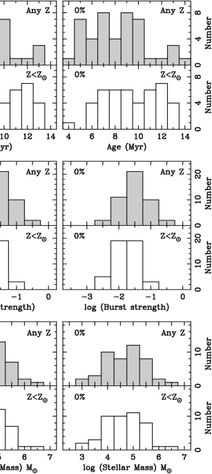
In Table 3 we show the mean age, burst strength, metallicity and stellar mass and their corresponding standard deviation values for all the star-forming regions studied. All those clusters of solutions with probability higher than 20 per cent are shown. This probability has been computed by dividing the number of Monte Carlo particles within a given cluster relative the total number of particles (10³). Using the mean value for the highest probability solution cluster of each star-forming region we obtained the frequency histograms shown in Fig. 2.

The results shown in Table 3 indicate that 50 per cent of the regions under study only show a cluster of solutions with probability higher than 20 per cent. In the remaining regions the mean differences obtained between the several solution clusters are 2.2 Myr, 0.15 dex and 0.14 dex in age, burst strength and mass, respectively, for models with a 15 per cent fraction of escaping photons and any metallicity. These differences are even lower by using other sets of models –1.8 Myr, 0.10 dex and 0.10 dex, respectively, for the subsolar metallicity models–. In any case, these differences are significantly lower than the dispersion observed in Fig. 2.

From Fig. 2 we also deduce that there is no large differences in the properties derived assuming 15 per cent or a null fraction of Lyman photons escaping from the nebula. If we compare the results obtained using subsolar metallicity models and those obtained for the whole range in metallicity, it seems that a higher number of regions older than 10 Myr and with burst strength lower than 1 per cent is obtained in the former case. Since the metallicity of the ionized gas (see Sect. 3.4) is clearly lower than solar, we are more confident with the results obtained using subsolar metallicity models. The Principal Component Analysis performed on the highest probability solution clusters indicate that the direction in the ($t$,$b$,$Z$) space that better reproduces the data variance is ($u_{t}$,$u_{b}$,$u_{Z}$)=($+$0.707,$+$0.707,0.000). This fact suggests the existence of a small degeneracy between age and burst strenght.

In the lower panels of Fig. 2 we show the stellar mass distribution. The stellar masses (see also Table 3) have been computed using the $K$-band absolute magnitudes measured within the apertures and the mean mass-to-light ratio of the highest-probability solution cluster. These stellar masses were corrected for the aperture effect by dividing them by the factors $f$ given in Table 3 (see Sect. 2.2).

Finally, the age, burst strength and mass values obtained for these regions are represented in Fig. 3 using different sized symbols. In Fig. 3a the size of the symbols used is related with the age of the burst, larger symbols represent younger regions. In Fig. 3b the symbol size is proportional to the burst strength, and finally, in Fig. 3c its size is proportional to the burst stellar mass. Figs. 2 and 3a show that the age of the star-forming regions is well constrained between 5-13 Myr. There is no significant age gradients across the different structures observed in the H$\alpha$ image (see Sect. 4).

It should be noticed that the age and burst strength values derived are not affected by the Mrk~86 distance uncertainty, since only aperture colors and equivalent widths have been used in this work.

Since we have adopted in our models a fixed mass-to-ligth ratio and colors for the underlying stellar population, the contamination from intermediate aged populations could yield sistematically higher age, burst strength and stellar mass values in some regions. This could be the case of the #45, #49 and #59 regions, contaminated from the central starburst continuum emission. On the other hand, the ignorance on the actual mass-to-light ratio of the underlying population, as we pointed out in Sect. 3.1, may introduce slight uncertainties in the stellar masses derived. However, although the absolute values for these masses would be quite uncertain, the relative differences should be similar.

3.4 Gas diagnostic for the star-forming regions

In Table 5 of Paper I we gave the emission-line fluxes measured in 4.30$\times$2.65 arcsec² regions centred in the maximum of the emission knot section covered by the slit.

The gas electron densities have been obtained from the [S ii]$\lambda$6716Å/[S ii]$\lambda$6731Å line ratio following Osterbrook (osterbrock (1989)). When the latter line ratio was not measurable we adopted an standard density of $n_{\mathrm{e}}$=100 cm^-3. In the cases where the ([O iii]$\lambda$4959Å$+$[O iii]$\lambda$5007Å)/[O iii]$\lambda$4363Å line ratio was measurable, we determined the electron temperatures applying the algorithms given by Gallego (gallego95 (1995)). The corresponding oxygen, nitrogen and helium abundances were also computed using the algorithms given by Gallego (gallego95 (1995)). Since the He ii$\lambda$4686Å emission-line fluxes were not measurable we could not determine the He iii abundance. In addition, since the [S iii]$\lambda\lambda$9069,9532Å emission lines were not accessible, we assumed a ionization correction factor of 1 and, consequently, $y$=$y^{+}$. A summary of the electron densities, temperatures and chemical abundances deduced is given in Table 4.

Finally, we have compared the line ratios measured with the predictions of a grid of model nebulae taken from Martin (martin97 (1997)) and originally calculated with cloudy. The nitrogen-to-oxygen and carbon-to-oxygen abundance ratios used were those employed by Martin (martin97 (1997)). The oxygen abundance was 0.2 (O/H)_☉.

In Fig. 4 the extinction corrected [O iii]$\lambda$5007Å/H$\beta$, [S ii]$\lambda\lambda$6717,6731Å/H$\alpha$, [O ii]$\lambda$3727Å/[O iii]$\lambda$5007Å and [N ii]$\lambda$6583Å/H$\alpha$ line ratios jointly with the models predictions have been plotted. We have drawn models with effective temperatures in the range 40000-50000 K and ionization parameters between log U=$-$1.91 and log U=$-$4.60. Solid-lines represent the change in the line ratios for different ionization parameter values between log U=$-$1.91 and $-$4.60 at increments of 4.7 in U. Thicker lines mean higher temperatures. The dashed-lines represent the change in the line ratios as a function of the effective temperature for a fixed ionization parameter. In all these diagrams the ionization parameter of the models increases from right to left. In Fig. 4a we also show the change in the line ratios measured along the major axis of the expanding bubble Mrk~86-B (GZG) from North to South (dotted-line).

Figure 4: Extinction corrected emission-line ratios. Only those regions with measurable Balmer decrements are shown. Photoionization models computed with cloudy are drawn for 50000, 45000 and 40000 K effective temperatures and ionization parameters between log U=$-$1.90 and $-$4.60. Solid-lines connect line ratios computed with different ionization parameters and fixed effective temperature. Thicker-lines mean higher temperatures. Dashed-lines connect predictions for different effective temperatures and fixed ionization parameter.

Figure 5: #26 and #27 regions. $B$, $R$, $Ks$ and H$\alpha$ images are shown. North is up and East is to the left. The scale is 0$\aas@@fstack{\prime\prime}$33 pixel^-1. The size of these images is approximately 0.4 kpc$\times$0.5 kpc.

As it was pointed out by Martin (martin97 (1997)), the bulk of the discrepancy of these line ratios with the prediction of photoionization models suggests the existence of an aditional excitation mechanism. This discrepancy will be higher using lower metallicity models. The contribution of this additional mechanism (or mechanisms) is more significant, relative to that produced by photoionization, in the case of the #45, #54 and #70 star-forming regions. In the latter case, the anomalous line-ratios measured are probably related with enhanced shocked gas emission in the Mrk~86-B bubble fronts (see GZG). The contamination from the Mrk~86-B north lobe could be also responsible for the line ratios measured in the #54 region.

3.5 Comments on several individual regions

#9, #10, #12, #22, #55, #57, #79, #84 and #85: All these regions show photometric H$\alpha$ emission, but very faint or undetectable $R$-band continuum emission. There are two feasible explanations for this very faint continuum emission.

First, these regions could be high gas density clumps photoionized by distant stellar clusters. Then, they should be placed in regions with intense diffuse H$\alpha$ emission. This could be the case of the #9, #10, #12, #22, #55 and #57 regions.

On the other hand, at the early evolutionary stages of a starburst the emission-line equivalent widths can be as high as 1000Å. Thus, star-forming regions with low burst strength will be only detectable by their H$\alpha$ or [O iii]$\lambda$5007Å emission. This could be the case of the #79, #84 and #85 regions.

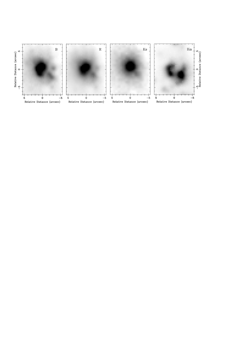
#26 & #27: These regions conform a massive association (see GZG) with very complex structure. The best-fitting model for the #26 region yields an age of about $\sim$10 Myr with a high burst strength value. On the other hand, the #27 region is a younger burst (5 Myr) with low burst strength and complex H$\alpha$ emission structure (see Fig. 5). The peculiar velocity profile obtained by GZG suggests that this association could belong to an independent stellar system merged with Mrk~86. In Fig. 5 we show the continuum and H$\alpha$ structure of this association. From this figure is not clear if the H$\alpha$ emission arises from photoionization of the #26, #27 or both stellar clusters. The H$\alpha$ fluxes of the #26 and #27 regions given in Table 5 of Paper I are those measured for the north-east and south-west structures shown in Fig. 5 (right panel), respectively.

#42, #70 & #18: These regions correspond to the starburst precursors of the Mrk~86-A, Mrk~86-B and Mrk~86-C expanding bubbles, respectively (see Martin martin (1998), GZG). From Fig. 3 we observe that these regions have extreme properties. In particular, the #70 region shows the highest burst strength (excepting #45 region and the central starburst) and the #18 region is the youngest of the regions analyzed in Sect. 3.3.

4 Global interpretation of the Mrk~86 star formation history

Summarizing, we have derived the properties of three well defined stellar populations;

1. Underlying population: Exponential surface profile, red colors, no significant color gradients. The ages derived range between 5 and 13 Gyr.

2. Central starburst: 20 per cent burst strength, 30 Myr old and total stellar mass of about 9$\times$10⁶ M_☉.

3. Star-forming regions: Low burst strengths ($\sim$2 per cent), ages between 5-13 Myr and low gas metallicities. No significant age or metallicity gradients are observed.

4.1 What has been ocurring during the last 30 Myr?

Most of the H ii regions in Mrk~86 are located in an bar oriented in north-south direction and placed 20″ west of the galactic center (see Fig. 3 and Fig. 2 of Paper I) and in an arc going from south-east (#58 & #64 regions) to north (#13 & #16 regions) of the central starburst. There is no significant age gradients across these structures, suggesting the existence of a large-scale triggering mechanism that activated the star formation simultaneously in most of these regions about 10 Myr ago.

We propose that the large-scale triggering mechanism for the recent star formation was produced by the growth of a superbubble originated at the galaxy central starburst by the energy deposition of stellar winds and supernova explosions. In some cases, local triggering mechanisms are also present. This could be the case of the complexes formed by the #26-#27, #26-#18, #58-#64 and #16-#13 regions. These complexes are constituted by an evolved burst (age$\geq$10 Myr) –the former–, and a very recent star-forming event, about 5 Myr old –the latter– (see Stewart et al. stewart (2000))

Hereafter, we will mainly focus on the large-scale triggering mechanism described above. Following the models of Silich & Tenorio-Tagle (silich (1998), STT hereafter; see also De Young & Heckman young94 (1994)), these collective supernova remnants grow at first elongated in the direction perpendicular to the galaxy disk. Due to this, the remnant blows out into the galaxy halo, leading to the formation of a secondary shell of swept out gas. About 20 Myr after the first supernova explosions (for the STT A100 model) the superbubble surrounds the inner densest part of the disk. Then, the leading shock, going through outer less dense regions, merges with its symmetrical counterpart. During this merging process a large fraction of swept out mass is strangled shaping a dense toroid. This region does not participate in the general outward motion, being strongly compressed towards the galaxy plane. As a result of this compression the activation of the star formation in the gas toroid could be produced if the mean surface density will be higher than 5-10 M_☉ pc^-2 (Skillman et al. skillman (1987); Kennicutt kenni89 (1989); see also Taylor et al. taylor94 (1994) for a sample of H ii galaxies).

The predictions described above correspond to the A100 model of STT. This model assumes a 10¹⁰ M_☉ massive galaxy with 10 per cent gas content, ISM central density of $n_{0}$=20.2 cm^-3, burst energy of $E_{\mathrm{burst}}$=10⁵⁶ erg and gas metallicity, Z=0.3 Z_☉. For this model, adopting a toroid width of 500 pc and a strangled mass of 2$\times$10⁸ M_☉, the surface density of the gas at the toroid will be about 64 M_☉ pc^-2. This value is intermediate between the gas surface densities measured in normal disks and in the infrared-seleted starbursts studied by Kennicutt (kenni98 (1998)). The galactocentric distance and epoch predicted for the formation of the toroid in the A100 STT model are 1.5 kpc and 25-30 Myr, respectively.

In the case of Mrk~86 the epoch for the formation of this toroid should be about 20 Myr (the age difference between the starburst and currently star-forming regions) at a radius of 0.8 kpc. Although these values well agree with the properties deduced for the A100 STT model, the high dependence of the evolution of the superbubble on the ISM density profile and the distance uncertainty for Mrk~86 prevent us to carry out a more quantitative analysis. However, this scenario provides a reliable and attractive explanation for the evolution of the star formation activity in Mrk~86.

Figure 6: Left-panel: VLA (D configuration) 21cm line intensity map courtesy of E. Wilcots. North is up and East is to the left. The edge-on spiral galaxy east-south of Mrk~86 is UGC~4278. The grey scale flux ranges between 0.025 and 3 kJy m s^-1 beam^-1 (see the upper bar on the figure). The beam size for this configuration is 46″(HPBW). Right-panel: $R$-band image obtained with the Wide-Field Camera (WFC) at the INT (see Paper I).

Finally, it should be noticed that the time since the formation of the toroid ($\sim$10 Myr) is significantly lower than the galaxy rotation period ($\sim$90 Myr), avoiding the disruption of this toroid by differential rotation. The galaxy rotation period was obtained using a projected angular velocity of 44 km s^-1 kpc^-1 and assuming an inclination of the rotation axis relative to the plane of the sky of 50^∘ (GZG; see also Gil de Paz gilphd (2000)).

The scenario described above is similar to that observed in other nearby dwarf star-forming galaxies. Thus, in the LMC the two arcs of stellar clusters place on the LMC4 superbubble rim round a population of 30 Myr old supergiants and Cepheid variables (Efremov & Elmegreen efremov (1998)). A similar study for the DEM192 superbubble also in the LMC was carried out by Oey & Smedley (oey (1998)).

4.2 What did happen 30 Myr ago?

Although we can accept that most of the recent star-forming activity in Mrk~86 was originated by a superbubble produced at the central starburst, we need to solve the question about the nature of the triggering mechanism of the star formation in the galaxy central starburst.

Under the evolutionary scenario described above, the observational properties of Mrk~86 about 30 Myr ago would be very similar to those of the nucleated Blue Compact Dwarfs (nE BCDs). It should show a very bright central starburst superimposed on an extended underlying component (see Papaderos et al. 1996a and references therein). This fact suggests the existence of an evolutionary connection between the different kinds of Blue Compact Dwarf galaxies. Therefore, the question about the star formation triggering in the central starburst of Mrk~86 is equivalent to the problem of the activation of the star formation in the BCD galaxy population as a whole.

Taylor et al. (taylor93 (1993)) hypothesized that the close passage of a companion galaxy has triggered the present burst of star formation (the central starburst in the Mrk~86 case) in many (if not all) of the BCD galaxies. These kind of distant encounters are well acepted to lead the lost of angular momentum in the gas component, resulting in the fall of large amounts of gas to the galaxy central regions (Barnes & Hernquist barnes92 (1992); Taylor et al. taylor94 (1994); Mihos & Hernquist mihos96 (1996)). This radial inflow will be very efficient in Mrk~86, because of the low dark matter content expected for this object (GZG; see Taylor taylor97 (1997)).

The first candidate for such a tidal interaction is NGC~2537A ($\alpha$(2000)=08^h13^m40.9^s $\delta$(2000)=$+$45°59′41″). However, the study of Heyd & Wiyckoff (heyd (1992)) and the 21cm line intensity map (see Fig. 6) show that this object is clearly a background galaxy. Then, the next candicate for the central starburst triggering is UGC~4278 ($\alpha$(2000)=08^h13^m58.8^s $\delta$(2000)=$+$45°44′36″), a nearly edge-on spiral galaxy placed at a projected distance of about 33 kpc relative to Mrk~86 (see Fig. 6). Its heliocentric velocity is 553 km s^-1 (Goad & Roberts goad (1981); see also Schneider & Salpeter schneider (1992)), and its radial velocity relative to the CMB is 715 km s^-1.

The offset of this galaxy relative to the Tully-Fisher template obtained by Giovanelli et al. (giovanelli97 (1997)) is 0.66^m in the $I$-band (R. Giovanelli, priv. comm.). Therefore, its peculiar radial velocity will be $-$253 km s^-1, being the radial velocity corrected for peculiar motions 968 km s^-1. Then, the distance to UGC~4278 could range between 13 and 19 Mpc, respectively for $h$=0.75 and 0.5. The large difference between this value and that derived by Sharina et al. (sharina99 (1999); see also Sect. 2.1 of Paper I) for Mrk~86 suggests that UGC~4278 is also a background galaxy.

Therefore, another triggering mechanism should be argued to explain the activation of the star formation in the Mrk~86 central starburst. This triggering mechanism could be related with the presence of previous massive star forming events. Our study has not revealed the existence of such an intermediate aged stellar population, probably excepting the #26 and #27 regions. As we indicated in Sect. 3.5 (see also GZG), the association constituted by the #26 and #27 regions shows a very steep velocity gradient that could be produced by the velocity field of an independent low mass system merged or in process of merging with Mrk~86. In that case, this merging process could be responsible for radial inflow of gas that led to the star formation activation in the central regions of Mrk~86. However, the large-scale distribution of neutral hydrogen in this galaxy (see Fig. 6; E. Wilcots, priv. comm.) indicates that, if this merging process took place, it should occur long time ago, probably several orbital periods ago.

5 Summary and conclusions

The main conclusions derived from this work are summarized hereafter.

• The Blue Compact Dwarf galaxy Mrk~86 is constituted by three well defined stellar populations. An evolved (5-13 Gyr old) stellar component characterized by an exponential light profile, no significant color gradients and low metallicity. A massive ($\sim$9$\times$10⁶ M_☉) central starburst, about 30 Myr old, with very low dust content and high burst strength ($\sim$20 per cent). And, finally, a young stellar population distributed in, at least, 46 star-forming regions. These star-forming regions are characterized by very low metallicities, burst strengths and stellar masses.

• The distribution of the star-forming regions properties suggest that their star formation triggering is related with a large-scale mechanism. Following the models of Silich & Tenorio-Tagle (silich (1998)), we propose that the growth of a superbubble produced by the energy deposition at the galaxy central starburst led to the formation of a dense toroid of ISM mass. Then, the high gas surface densities reached produced the activation of the current star-forming activity.

• Finally, we studied the possible triggering mechanisms for the activation of the star formation in the galaxy central starburst. Since both candidates for a distant encounter, NGC~2537A and UGC~4278, seem to be background galaxies, the merging with a low mass companion seems the most feasible explanation for this central starburst activation.

References

- (1) Aloisi A., Tosi M., Greggio L., 1999, AJ 118, 302
- (2) Arp H., 1966, Atlas of Peculiar Galaxies. California Institute of Technology, Pasadena
- (3) Barnes J.E., Hernquist L.E., 1992, ARA&A 30, 705
- (4) Bruzual A.G., 1983, ApJ 273, 105
- (5) Burkert A., 1989, Ph.D. Thesis, Munich
- (6) Burstein D., Heiles C., 1982, AJ 87, 1165
- (7) Calzetti D., Kinney A.L., Storchi-Bergmann T., 1996, ApJ 458, 132
- (8) Campbell A.W., Terlevich R., 1984, MNRAS 211, 15
- (9) De Young D.S., Heckman T.M., 1994, ApJ 431, 598
- (10) Doublier V., 1998, Ph.D. Thesis, Marsella
- (11) Drinkwater M., Hardy E., 1991, AJ 101, 94
- (12) Efremov Y.N., Elmegreen B.G., 1998, MNRAS 299, 643
- (13) Fanelli M.N., O’Conell R.W., Thuan T.X., 1988, ApJ 334, 665
- (14) Gallego J., 1995, Ph.D. Thesis, Universidad Complutense de Madrid
- (15) Gil de Paz A., 2000, Ph.D. Thesis, Universidad Complutense de Madrid
- (16) Gil de Paz A., Zamorano J., Gallego J., 1999, MNRAS 306, 975 (GZG)
- (17) Gil de Paz A., Zamorano J., Gallego J., Domínguez F. de B., 2000a, A&A (Paper I)
- (18) Gil de Paz A., Aragón-Salamanca A., Gallego J., et al., 2000b, MNRAS 316, 357
- (19) Giovanelli R., Haynes M.P., Herter T., et al., 1997, AJ 113, 53
- (20) Goad J.W, Roberts M.S., 1981, ApJ 250, 79
- (21) Gorgas J., Faber S.M., Burstein D., et al., 1993, ApJS 86, 153
- (22) Gorgas J., Cardiel N., Pedraz S., González J., 1999, A&AS 139, 29
- (23) Heyd R., Wyckoff S., 1992, BAAS 181, #45.09
- (24) Hoffman G.L., Salpeter E.E., Helou G., 1990, in the proceedings of the Edwin Hubble Centennial Symposium, 67
- (25) Kennicutt R.C., 1989, ApJ 344, 685
- (26) Kennicutt R.C., 1998, ApJ 498, 541
- (27) Kunth D., Sargent W.L.W., 1986, ApJ 300, 496
- (28) Kunth D., Maurogordato S., Vigroux L., 1988, A&A 204, 10
- (29) Loose H.-H., Thuan T.X., 1985, The Morphology and Structure of BCDGs from CCD Observations, in: Kunth, D., Thuan, T.X., and Van, J.T.T.(eds.) Star-Forming Dwarf Galaxies. Editions Frontières.
- (30) Markarian B.E., 1969, Astrofizika, 5, 443
- (31) Marlowe A.T., Heckman T.M., Wyse R.F.G., Schommer R., 1995, 438, 563
- (32) Martin C.L., 1997, ApJ 491, 561
- (33) Martin C.L., 1998, ApJ 506, 222
- (34) Mihos J.C., Hernquist L., 1996, ApJ 464, 641
- (35) Morrison D.F., 1976, Multivariate Statistical Methods, McGraw-Hill Book Co., Singapore
- (36) Murtagh F., Heck A., 1987, Multivariate Data Analysis, D. Reidel Publishing Co., Dordrecht, Holland
- (37) Norton S., Salzer J.J., 1997, BAAS 190
- (38) Oey M.S., Smedley S.A., 1998, AJ 116, 1263
- (39) Osterbrock D.E., 1989, Astrophysics of Gaseous Nebulae and Active Galactic Nuclei. University Science Books, Mill Valley, California.
- (40) Papaderos P., Loose H.-H., Thuan T.X., Fricke K.J., 1996a, A&AS 120, 207
- (41) Papaderos P., Loose H.-H., Fricke K.J., Thuan T.X., 1996b, A&A 314, 59
- (42) Schneider S.E., Salpeter E.E., 1992, ApJ 385, 32
- (43) Searle L., Sargent W.L.W., 1972, ApJ 173, 25
- (44) Searle L., Sargent W.L.W., Bagnuolo W.G., 1973, ApJ 179, 427
- (45) Shapley H., Ames A., 1932, Ann. Harvard College Obs. 88, No. 2
- (46) Sharina M.E., Karachentsev I.D., Tikhonov N.A., 1999, Astronomy Letters 25, 322
- (47) Silich S.A., Tenorio-Tagle G., 1998, MNRAS 299, 249 (STT)
- (48) Silk J., Wyse R.F.G., Shields G.A., 1987, ApJ 322, L59
- (49) Skillman E.D., Bothun G.D., Murray M.A., Warmels R.H., 1987, A&A 185, 61
- (50) Stewart S.G., Fanelli M.N., Byrd G.G., et al., 2000, ApJ 529, 201
- (51) Taylor C.L., 1997, ApJ 480, 524
- (52) Taylor C.L., Brinks E., Skillman E.D., 1993, AJ 105, 128
- (53) Taylor C.L., Brinks E., Pogge R.W., Skillman E.D., 1994, AJ 107, 971
- (54) Thuan T.X., 1983, ApJ 268, 667
- (55) Thuan T.X., 1991, Observations and Models of Blue Compact Dwarf Galaxies, in: Leitherer C., Walborn R.N., Heckman T.M., Norman C.A. (eds.) Massive Stars in Starbursts, Cambridge University Press, p.183.
- (56) Thuan T.X., Martin G.E., 1981, ApJ 247, 823
- (57) Worthey G., 1994, ApJS 95, 107