Mapping the star formation history of Mrk~86^∗

Abstract

We have obtained optical ($BVR$, [O iii]$\lambda$5007Å and H$\alpha$), near infrared ($JHK$) imaging and long-slit optical spectroscopy for the Blue Compact Dwarf galaxy Mrk~86 (NGC~2537). In this paper, the first of two, we present optical-near-infrared colors and emission-line fluxes for the currently star-forming regions, intemediate aged starburst and underlying stellar population. We also describe the evolutionary synthesis models used in Paper II.

The $R$ and H$\alpha$ luminosity distributions of the galaxy star-forming regions show maxima at $M_{R}$=$-$9.5^m and $L_{\mathrm{H}\alpha}$=10^37.3 erg s^-1. The underlying stellar population shows an exponential surface brigthness profile with central value, $\mu_{\mathrm{E,0}}$=21.5 mag arcsec^-2, and scale, $\alpha$=0.88 kpc, both measured in the $R$-band image. In the galaxy outer regions, dominated by this component, no significant color gradients are observed.

Finally, a complete set of evolutionary synthesis models have been developed, covering a wide range in metallicity, 1/50 Z_☉$<$Z$<$2 Z_☉, and burst strength, 1-10^-4. These models include nebular continuum and recombination and forbidden-line emission.

1 Introduction

The high star formation rate (SFR hereafter) and low neutral gas content deduced for dwarf star-forming galaxies imply consumption time-scales of about 10⁹ yr (Fanelli et al. fanelli (1988); Thuan & Martin thuan81 (1981)), much shorter than the age of the Universe. Searle et al. (searle73 (1973)) suggested that either these objects are truly young systems or they have an intermittent star formation history with short intense star-forming episodes followed by long quiescent phases. Although this question remained unanswered during decades (Thuan thuan83 (1983); Campbell & Terlevich campbell (1984); Loose & Thuan loose85 (1985)), nowadays, most of the studies on dwarf star-forming systems, including Blue Compact Dwarf galaxies (BCD hereafter), have revealed the existence of an evolved underlying population (Kunth et al. kunth88 (1988); Hoffman et al. hoffman (1990); Papaderos et al. 1996b ; Doublier doublier98 (1998); Norton & Salzer norton (1997)).

Therefore, the understanding of the mechanism, or mechanisms, governing this star formation regulation is the stepping stone of the dwarf star-forming galaxies evolution. Moreover, this mechanism constitutes the missing link between the different dwarf star-forming galaxies (Silk et al. silk87 (1987); Burkert burkert (1989); Drinkwater & Hardy drinkwater (1991); Papaderos et al. 1996b ).

There are two different approaches to address these questions. On the one hand, statistical analysis of a sample of these objects will allow the study of the relationships between fundamental parameters and properties of the star-forming dwarf galaxies (Marlowe et al. marlowe95 (1995); Papaderos et al. 1996a , 1996b ). On the other hand, the detailed analysis of individual low-redshift objects with multiple regions of star formation is fundamental to reconstruct their star formation histories. In particular, we can obtain a better understanding of possible effects of merging or some internal process as self-propagation that could originate the spreading of star formation, and the effects of these star-forming events on the future star formation.

Among dwarf galaxies, Blue Compact Dwarf galaxies conform the subpopulation where the star-forming events are most violent. Blue Compact Dwarfs are low-luminosity (M_B $\geq$$-$18^m) galaxies with compact sizes whose spectra are similar to those of low metallicity H ii regions (Searle & Sargent searle72 (1972); Kunth & Sargent kunth86 (1986); Thuan & Martin thuan81 (1981)). Their spectra are characterized by emission lines over a blue continuum which implies the existence of a large fraction of OB stars and an intense star-forming activity.

The Blue Compact Galaxy Mrk~86=NGC~2537 (Shapley & Ames shapley32 (1932); Markarian markarian69 (1969)), also known as Arp 6 (Arp arp66 (1966)), constitutes an excellent laboratory to test the BCD star formation history since its star-forming regions populate all the galaxy. This object is the propotype of the iE galaxies, the most important BCD galaxies subclass, that conform 70 per cent of the BCD galaxies (Thuan & Martin thuan81 (1981); Thuan thuan91 (1991)).

Optical imaging (both broad- and narrow-band) and near infrared images have been obtained to map the different regions and get insight into the star formation history of every region. In addition, we have obtained very high quality spectra with spatial resolution. The spectra of 22 star-forming knots and of free interim were taken with 10 distinct slit positions and orientations and moderate and high spectral resolution.

After briefly introduce the previous results on Mrk~86 in Sect. 2, we will describe the observations and data reduction in Sect. 3. The data analysis is presented in Sect. 4. We describe the evolutionary synthesis models in Sect. 5. In Sect. 6 we give some results. Finally, our conclusions are presented in Sect. 7.

In Gil de Paz et al. (2000a ; Paper II hereafter) we derive the physical properties of the star-forming regions and stellar populations of Mrk~86 comparing our photometric data with the evolutionary synthesis models presented in this paper. Electron densities and temperatures and chemical abundances of the ionized gas in the galaxy star-forming regions will be also obtained. Finally, a global interpretation of the galaxy will be given.

Table 1: Collection of the published parameters of Mrk~86

Parameter	Data	Reference
v☉	447 km s-1	(1)
vLG	522 km s-1	(1)
vLG	460 km s-1	(2)
Distance	6.9 Mpc	(3)
$B$	12.8	(4)
f(1510Å)	0.87$\times$10-14 erg m-2 s-1 Å-1	(5)
S(2.8cm)	7$\pm$2 mJy	(6)
S(6.3cm)	18$\pm$4 mJy	(7)
S(1.2cm)	11$\pm$4 mJy	(7)
f(12$\mu$m)	0.25 Jy	(8)
f(25$\mu$m)	0.42 Jy	(8)
f(60$\mu$m)	3.15 Jy	(8)
f(100$\mu$m)	6.26 Jy	(8)
$L_{\mathrm{IR}}$	0.35 109 L☉	(8)
$J$	13.25	(9)
$H$	12.57	(9)
$K$	12.37	(9)
$L$	12.63	(9)
M(H i)	2.4 108 M☉	(10)
MT	5.8 108 M☉	(10)
f(H i 21cm)	2.1 Jy km s-1	(11)
FWHM${}_{\mathrm{{H\textsc{i}}}}$	93 km s-1	(11)
ICO	0.83$\pm$0.12 K km s-1	(12)

(1) Bottinelli et al. (bottinelli90 (1990)); (2) Rood & Dickel (rood76 (1976)); (3) Sharina et al. (sharina (1999)); (4) Dultzin-Hacyan et al. (dultzin90 (1990)); (5) Fanelli et al. (fanelli (1988)); (6) Klein et al. (klein91 (1991)); (7) Klein et al. (klein84 (1984)); (8) Thronson & Telesco (thronson86 (1986)); (9) Thuan (thuan83 (1983), measured with 7$\aas@@fstack{\prime\prime}$8 apertures); (10) Thuan & Martin (thuan81 (1981)); (11) Verter (verter (1985)); (12) Sage et al. (sage92 (1992)).

2 Mrk 86

Mrk~86 ($\alpha$(2000)=08^h13^m14.56^s $\delta$(2000)=$+$45°59′30.2″) is a well-known object among BCD galaxies (Loose & Thuan loose85 (1985); Sage et al. sage92 (1992); see Table 1). In the Loose & Thuan (loose85 (1985)) BCD classification, Mrk~86 belongs to the iE class: smooth elliptical Low Surface Brightness (LSB) underlying stellar component on which several knots of star formation are superimposed. The present star formation activity is spread out in several clumps over a relatively large fraction of its entire surface. In fact, Mrk~86 shows the highest ratio of the area covered by star-forming regions to the total projected area of the galaxy within the sample of Papaderos et al. (1996a ).

To this moment Mrk~86 has not been the subject of a single and proof study, inasmuch the large number of published data on it. A collection of the published data is given in Table 1. A more detailed description of the previous observations is given by Gil de Paz et al. (gil1 (1999); GZG hereafter).

2.1 Distance

Mrk~86 is a nearby star-forming galaxy. The heliocentric recession velocity is $v_{\sun}$=447 km s^-1 (see recession velocities referred to the Local Group in Table 1).

Using the mean blue magnitude of the three brightest blue stars Sharina et al. (sharina (1999)) derived a distance for this object of 6.9 Mpc with an uncertainty of 20 per cent (M. E. Sharina, private communication). We can also estimate the distance to Mrk~86 if we assume that it is gravitationally bounded to the edge-on spiral galaxy UGC~4278 (see Paper II). UGC~4278 has a corrected $I$-band absolute magnitude of $-$18.21$\pm$0.11 (see Giovanelli et al. giovanelli97 (1997)) with a logarithmic 21 cm line width of 2.220$\pm$0.019 (in km s^-1). Therefore, with respect to the Giovanelli et al. (giovanelli97 (1997)) Tully-Fisher template, this galaxy shows an offset of 0.66^m, which corresponds to a peculiar radial velocity of $-$253 km s^-1. Thus, its recesion velocity in the CMB reference frame should be 968 km s^-1 ($v_{\sun}$=565 km s^-1), which implies a minimum distance for Mrk~86 of 13 Mpc (for $H_{0}$=75 km s^-1 Mpc^-1 and assuming that the difference in heliocentric velocity is due to orbital motion). The large difference between this value and that given by Sharina et al. (sharina (1999)) suggests that these objects are probably not physically bounded. Thus, since no other distance indicator is available for Mrk~86, we have used the distance measured by Sharina et al. (sharina (1999)) throughout this work. This value leads a projected spatial scale of 33 pc arcsec^-1.

3 Observations and reduction

3.1 Optical imaging

An optical $B$-band image was obtained at the 1-m Jacobus Kapteyn Telescope (JKT) of Roque de los Muchachos observatory (La Palma, Spain) in 1997 November with a 24 $\mu$m 1024$\times$1024 pixels Tek#4 CCD (see Table 2). An additional Johnson-$V$ image was taken at the 1.52-m spanish telescope at EOCA (Calar Alto, Almería, Spain) in December 1993 with a Tek 1024$\times$1024 CCD with pixel size of 19 $\mu$m. This observation was broken up into five exposures with a total integration time of 2400 s. Finally, an $R$-band image was obtained during service time in November 1998 with the ING wide-field camera (ING-WFC) equipped with four EEV42 2k$\times$4k pixels CCD detectors on the 2.5-m Isaac Newton Telescope (La Palma, Spain).

Narrow-band images in the light of [O iii]$\lambda$5007Å ($\lambda_{0}$ = 5012Å, FWHM = 50Å) and H$\alpha$ ($\lambda_{0}$ = 6568Å, FWHM = 95Å) were obtained. In order to subtract the continuum, $V$ and $R$-band images were used, respectively. The [O iii]$\lambda$5007Å image was secured for us on December 1993 during service time with a 1280$\times$1180 pixels EEV5 CCD attached to the 2.5-m Isaac Newton Telescope. The H$\alpha$ image was taken during the same service time observations that the $R$-band image in November 1998 using the ING-WFC camera at the 2.5-m Isaac Newton Telescope (La Palma, Spain).

High S/N ratio dome flats and exposures of the sky taken in twilight were obtained in any case. The standard procedure of bias removal, dark-current subtraction, and flat fielding using dome and sky flat-field images was performed using the ESO image processing system MIDAS for the $V$ image and IRAF for the $B$ and $R$-band images.

Atmospheric conditions were photometric during the observing runs. $B$ and $V$ images were flux calibrated observing repeatedly during the nights a set of standard stars, taken from the lists given by Kent (kent (1985)) and Landolt (landolt (1973)). Finally, the $R$-band image was flux calibrated using the radial surface brightness profile published by Papaderos et al. (1996a ).

The [O iii]$\lambda$5007Å and H$\alpha$ images flux calibration was performed as follows (see also GZG). The continuum emission was subtracted, using the $V$ and $R$ images, respectively. Then, we trimmed those regions covered by the slits of the $b$(blue) and $r$(red) spectra (see Table 2). The $b$ and $r$ spectra were convolved with the transmission curves of the corresponding narrow-band filters. Then, we compared image counts and fluxes measured in the convolved spectra for several adjacent regions in order to determine the precise location of the slits. Finally, once the regions covered by the slits were precisely defined, we corrected these calibration relations for the sensitivity of the filter at the corresponding wavelength and, in the case of the H$\alpha$ flux, for the contribution of the [N ii]$\lambda$6548Å and [N ii]$\lambda$6583Å lines. The discrepancies obtained among different spectra were in all cases lower than 10 per cent.

Table 2: Journal of observations.

	Spectroscopic Observations†
	Exp.	Slit	Range	Disp.
Telescope	time(s)		(nm)	(Å/pix)
CAHA2.2m	3600	#1,2,4,6$b$	330-580	2.6
CAHA2.2m	1800	#5$b$	330-580	2.6
CAHA2.2m	3600	#1,2,4,5,6$r$	435-704	2.6
CAHA2.2m	3600	#3	390-650	2.6
INT2.5m	1800	#7,8R	637-677	0.39
INT2.5m	900	#9R	637-677	0.39
	Image Observations
	Exp.	Filter	Scale	PSF
Telescope	time(s)		(″/pixel)	(″)
JKT1.0m	600	$B$	0$\aas@@fstack{\prime\prime}$33	1$\aas@@fstack{\prime\prime}$0
CAHA1.5m	2400	$V$	0$\aas@@fstack{\prime\prime}$33	1$\aas@@fstack{\prime\prime}$6
INT2.5m	900	$R$	0$\aas@@fstack{\prime\prime}$333	1$\aas@@fstack{\prime\prime}$2
INT2.5m	900	[O iii]$\lambda$5007	0$\aas@@fstack{\prime\prime}$57	2$\aas@@fstack{\prime\prime}$5
INT2.5m	7200	H$\alpha$	0$\aas@@fstack{\prime\prime}$333	1$\aas@@fstack{\prime\prime}$2
KPNO2.3m	900	$J$	0$\aas@@fstack{\prime\prime}$66	1$\aas@@fstack{\prime\prime}$8
KPNO2.3m	360	$H$	0$\aas@@fstack{\prime\prime}$66	1$\aas@@fstack{\prime\prime}$6
KPNO2.3m	540	$K$	0$\aas@@fstack{\prime\prime}$66	1$\aas@@fstack{\prime\prime}$7

^† See Fig. 1 of GZG for slit orientations and positions.

Figure 1: $BVRJHK$, H$\alpha$ and [O iii]$\lambda$5007Å images of Mrk~86.

Figure 2: Knot contours derived using the cobra program superimposed on the H$\alpha$ image. The $thick$-$lined$ contour corresponds to the starburst component as described by Papaderos et al. (1996a , see Sect. 6.3). The crossed-circle position marks the center of the outer $R$-band isophotes.

3.2 Near-infrared imaging

Near-infrared images (nIR hereafter) of Mrk~86 in $J$ ($\lambda_{0}$ = 1.25$\mu$m, FWHM = 0.30$\mu$m), $H$ ($\lambda_{0}$ = 1.65$\mu$m, FWHM = 0.28$\mu$m) and $Ks$ ($\lambda_{0}$ = 2.15$\mu$m, FWHM = 0.33$\mu$m) were obtained on January 1998 with the Steward Observatory near-infrared camera equipped with a 256$\times$256 nicmos3 detector attached to the 2.3-m Bok Telescope at Kitt Peak National Observatory (Arizona, USA). The observational procedure closely follows that of Aragón-Salamanca et al. (aas93 (1993)) and Gil de Paz et al. (2000b ). The total integration time of each subimage was broken up into background-limited sub-exposures to avoid saturation of the detector. Images of adjacent blank areas of the sky were alternated with the target frames for accurate flat-fielding. Comparable amounts of time were spent imaging the source and the sky to ensure adequate monitoring of the sky changes. Individual subexposures of the object were offset several arcseconds to improve the final result.

The reduction process include: (1) bias and dark subtraction of object and sky frames; (2) flat-fielding using normalized sky frames; (3) sky subtraction using sky frames taken before and after each exposure; (4) bad pixel removal; (5) registering of the subimages using fractional pixel shifts and (6) median combining of all individual frames. The reduction was carried out using own IRAF procedures.

Figure 3: Surface brightness profiles in the $BVRJHK$ bands. The fit to the exponential component of the $R$-band profile at distances larger than 70″ is also drawn. Error bars represent $\pm$1$\sigma$. The $K$-band profile has been offset $-$0.5^m in order to avoid confusion with the $H$-band profile.

The nIR images were calibrated observing standard stars from the list from Elias et al. (elias (1982)) during the nights at the same airmasses than the object. We have assumed a color independent correction between the $Ks$ and $K^{\prime}$ bands ($K^{\prime}\equiv KM$; $\lambda_{0}$ = 2.12$\mu$m, FWHM = 0.34$\mu$m; Wainscoat & Cowie wainscoat (1992)). In order to check the validity of this assumption, we convolved the $Ks$ and $K^{\prime}$ filters response functions with Planck spectral distributions at different temperatures in the range 3000-20000 K, obtaining the fluxes $F_{Ks}$ and $F_{K^{\prime}}$. The larger difference in 2.5$\times$log($F_{Ks}$/$F_{K^{\prime}}$) within this temperature range was 0.025^m, small enough to assume this correction to be independent of the spectral energy distribution.

Thus, once the fluxes were transformed to $K^{\prime}$-band fluxes, we converted them to the standard $K$-band ($\lambda_{0}$ = 2.19$\mu$m, FWHM = 0.41$\mu$m) applying the standard correction given by Wainscoat & Cowie (wainscoat (1992)), $K^{\prime}-K$=0.22$\times$($H-K$).

In Fig. 1 we show the Mrk~86 neighborhood in the optical-near-infrared bands studied, including the H$\alpha$ and [O iii]$\lambda$5007Å images. The astrometric calibration was performed using the program PlateAstrom (García-Dabó & Gallego dabo (1999); see also http://www.ucm.es/info/Astrof/opera/opera.html). The bright field star placed at the relative position (60″E,30″N), saturated in the $V$ and $R$-band images, was artificially removed.

3.3 Spectroscopy

Up to 14 optical long-slit spectra at 10 different slit positions were obtained. The 11 medium-low resolution spectra ($b$ and $r$ spectra; see Table 2) were obtained with the Boller & Chivens spectrograph at the Cassegrain focus of the 2.2-m telescope at the German-Spanish Calar Alto observatory (Almería, Spain) in January 1993. Althought special care was taken to place the slits into position, using offsets from the bright field star at north of the galaxy, there were some lack of precision. The actual positions of the slits (see Fig. 1 of GZG) were determined a posteriori comparing broad-band image spatial cuts with the spatial profiles of the spectra previously convolved with the corresponding filter transmission curves. The detector employed was a 1024$\times$1024 Tek#6 CCD with a pixel size of 24 $\mu$m. The 600 gr mm^-1 grating chosen provided a spectral resolution of 6Å in the light of H$\alpha$ and a reciprocal dispersion of 2.6Å/pixel, with a slit width of 2$\aas@@fstack{\prime\prime}$65. The final spatial scale was 1$\aas@@fstack{\prime\prime}$43/pixel. The spectral coverage was around 2500Å and the grating angle was selected to cover the blue region ($\sim$3300-5800Å) and red domain ($\sim$4350-7045Å) in two different exposures which overlapped on the H$\beta$ region. The seeing was variable during the observing run with FWHM between 1$\aas@@fstack{\prime\prime}$5–2$\aas@@fstack{\prime\prime}$5. The low airmasses at which these spectra were obtained ($\leq$1.2) guarantee that no significant loss of blue light due to atmospheric refraction has ocurred. In addition, three high resolution spectra (7R,8R,9R) were obtained with the IDS spectrograph at the Isaac Newton Telescope (INT) of the Roque de los Muchachos Observatory (La Palma, Spain) in January 1998 with a 1024$\times$1024 Tek#3 24 $\mu$m CCD (see Table 2). The 1200R grating (1200 gr mm^-1) was used with an slit width of 1″, providing a spectral resolution of 0.9Å in the light of H$\alpha$ and a reciprocal dispersion of 0.39Å/pixel. The spatial scale was of 0.33″/pixel.

These spectra were reduced using the figaro (January 1993) and IRAF (January 1998) software packages. After bias removal and flat-fielding, the frames were cleaned of cosmic rays. The sky was removed from each frame by subtracting a polynomial fitted to those regions free for object emission. Wavelength calibration was performed by using He-Ar lamps observed inmediately before and after the galaxy integration. The standard stars Hiltner 102 and Hiltner 600 were observed at different airmasses in order to correct for atmospheric extinction and to ensure absolute flux calibration.

Finally, we requested an UV spectrum of Mrk~86 from the International Ultraviolet Explorer (IUE) Final Archive (see Fig. 4). It was originally taken by Alloin and Duflot in January 1983 (see Bonatto et al. bonatto (1999)). The total exposure time of this spectrum, SWP18927, was 24000 s. It was obtained in low dispersion mode with the SWP camera. In the observing spectral range, 1150-1975Å, the resolution power varies between 270-300 (Cassatella et al. cassatella (1985)).

4 Analysis

4.1 Surface brightness profiles

We have analyzed the surface brightness profile of Mrk~86 in different bands ($BVRJHK$; see Fig. 3). These surface brightness profiles have been obtained using the IRAF task ellipse. Background galaxies and foreground stars were interactively masked. We obtained the surface brightness profiles over the original images, excepting in the outer regions of the $R$-band profile where a median filter of 5$\times$5 pixels (0$\aas@@fstack{\prime\prime}$333/pixel) was applied. Due to the contribution of about 60 high surface brightness regions, we only fitted the isophotes with major axis larger than 25″. Using the mean of the isophotal centers measured between 80 and 120″ in the $R$-band image we have estimated the galaxy coordinates given in Sect. 2 (see also Fig. 2).

4.2 Knot positions and sizes

Table 3: Positions and sizes for the Mrk~86 neighborhood regions.

#   #’	RA(2000)	DEC(2000)	$r_{1e}$  $r_{1e}$’	$e$	Cl.
(1)  (2)	(3)	(4)	(5)  (6)	(7)	(8)
01     –	08:13:16.08	$+$46:00:17.1	0.71 PLR	2	B
02     –	08:13:16.33	$+$46:00:12.1	0.85 0.45	1	B
03     –	08:13:15.91	$+$46:00:11.8	0.74 0.17	2	B
04     01	08:13:14.72	$+$46:00:04.1	1.13 0.87	2	F
05     –	08:13:13.38	$+$46:00:01.7	0.91 0.56	2	B
06     02	08:13:12.36	$+$45:59:57.6	1.07 0.79	2	E
07     –	08:13:15.70	$+$45:59:57.4	0.83 0.41	2	E
08     03	08:13:16.18	$+$45:59:56.0	0.96 0.63	2	E
09†   –	08:13:15.28	$+$45:59:54.1	0.76 0.24	2	E
10†   –	08:13:13.56	$+$45:59:53.4	0.68 PLR	1	E
11     04	08:13:12.20	$+$45:59:53.0	0.75 0.21	2	B
12†   –	08:13:16.74	$+$45:59:52.9	1.06 0.78	2	E
13     05	08:13:14.36	$+$45:59:52.0	1.31 1.09	1	E
14     06	08:13:11.72	$+$45:59:50.7	1.36 1.15	2	S
15     08	08:13:13.85	$+$45:59:50.7	0.96 0.63	2	E
16     07	08:13:14.77	$+$45:59:50.6	1.72 1.56	1	S
17     –	08:13:09.23	$+$45:59:49.5	1.03 0.74	2	E
18     09	08:13:13.08	$+$45:59:48.2	0.93 0.59	2	S
19     10	08:13:15.02	$+$45:59:45.3	1.56 1.38	1	S
20     11	08:13:15.33	$+$45:59:45.2	2.29 2.17	1	S
21     12	08:13:15.78	$+$45:59:44.8	0.88 0.51	1	E
22†   13	08:13:13.52	$+$45:59:44.2	1.02 0.72	2	E
23     14	08:13:10.94	$+$45:59:43.0	0.97 0.65	2	E
24     –	08:13:08.52	$+$45:59:41.4	1.19 0.95	2	E
25     –	08:13:15.64	$+$45:59:41.2	1.39 1.19	2	N
26     15	08:13:13.13	$+$45:59:40.6	2.11 1.98	2	S
27     16	08:13:12.94	$+$45:59:38.4	1.32 1.11	1	S
28†   17	08:13:13.64	$+$45:59:36.9	0.84 0.43	2	E
29     18	08:13:15.51	$+$45:59:35.6	0.85 0.45	2	S
30     19	08:13:15.92	$+$45:59:35.6	0.93 0.59	2	E
31     20	08:13:12.87	$+$45:59:35.1	0.65 PLR	2	N
32     21	08:13:13.41	$+$45:59:34.3	0.69 PLR	2	S
33     22	08:13:16.11	$+$45:59:33.9	0.96 0.63	1	E
34     –	08:13:08.99	$+$45:59:33.0	1.32 1.11	2	E
35     23	08:13:13.69	$+$45:59:33.0	1.28 1.06	2	N
36     24	08:13:13.28	$+$45:59:32.4	0.71 PLR	2	N
37     26	08:13:15.88	$+$45:59:29.3	1.90 1.76	1	S
38     27	08:13:16.23	$+$45:59:29.2	0.94 0.60	2	N
39     28	08:13:17.76	$+$45:59:29.0	1.20 0.96	2	B
40     25	08:13:12.76	$+$45:59:28.8	1.62 1.45	2	S
41     29	08:13:14.04	$+$45:59:27.3	1.07 0.79	2	S
42     31	08:13:12.98	$+$45:59:26.5	1.29 1.07	1	S
43     32	08:13:16.77	$+$45:59:25.9	1.12 0.86	1	E
44     33	08:13:12.63	$+$45:59:24.6	0.79 0.33	2	N
45     –	08:13:14.57	$+$45:59:23.2	1.15 0.90	2	S
46     34	08:13:12.37	$+$45:59:22.3	1.03 0.74	2	N
47     36	08:13:16.76	$+$45:59:21.2	1.22 0.98	1	S
48     35	08:13:12.69	$+$45:59:21.2	1.18 0.93	1	E
49     –	08:13:15.36	$+$45:59:18.8	0.73 0.12	2	N
50     37	08:13:11.19	$+$45:59:18.8	1.42 1.22	2	E
51     38	08:13:12.72	$+$45:59:17.3	1.28 1.06	2	N
52     39	08:13:12.97	$+$45:59:17.2	1.32 1.11	2	S
53†   –	08:13:13.64	$+$45:59:17.1	0.86 0.47	2	E
54     40	08:13:14.91	$+$45:59:15.9	2.01 1.88	1	S
55†   –	08:13:16.12	$+$45:59:15.8	0.69 PLR	2	E
56     –	08:13:17.35	$+$45:59:14.6	0.81 0.37	2	E

Table 3: (cont.) Positions and sizes for the Mrk~86 neighborhood regions.

#   #’	RA(2000)	DEC(2000)	$r_{1e}$  $r_{1e}$’	$e$	Cl.
(1)   (2)	(3)	(4)	(5)  (6)	(7)	(8)
57†   –	08:13:16.05	$+$45:59:13.1	0.82 0.39	2	E
58     41	08:13:16.84	$+$45:59:12.3	1.00 0.69	2	E
59     44	08:13:15.25	$+$45:59:11.6	0.86 0.47	2	S
60     43	08:13:18.27	$+$45:59:11.4	0.86 0.47	2	E
61     42	08:13:14.39	$+$45:59:11.4	0.77 0.27	3	F
62     –	08:13:16.04	$+$45:59:09.8	1.28 1.06	1	S
63     –	08:13:12.48	$+$45:59:09.4	0.56 PLR	2	N
64     45	08:13:16.74	$+$45:59:08.7	1.30 1.08	1	E
65     –	08:13:17.60	$+$45:59:07.6	1.22 0.98	1	E
66     46	08:13:13.05	$+$45:59:07.0	1.47 1.28	2	S
67     47	08:13:15.94	$+$45:59:06.9	0.80 0.35	3	F
68     –	08:13:13.75	$+$45:59:05.9	0.62 PLR	2	E
69     48	08:13:11.94	$+$45:59:05.2	0.95 0.62	2	B
70     49	08:13:14.28	$+$45:59:02.8	1.43 1.24	2	S
71     –	08:13:15.81	$+$45:59:02.6	0.75 0.21	2	N
72     50	08:13:15.68	$+$45:59:02.0	1.05 0.76	2	N
73     –	08:13:09.67	$+$45:59:00.6	1.08 0.80	2	B
74     –	08:13:15.52	$+$45:58:59.0	1.08 0.80	2	E
75     –	08:13:15.07	$+$45:58:53.5	0.95 0.62	2	E
76†    –	08:13:14.36	$+$45:58:52.3	1.11 0.84	1	E
77     –	08:13:17.80	$+$45:58:52.1	0.87 0.49	2	E
78     –	08:13:12.32	$+$45:58:48.3	1.03 0.74	1	E
79†    –	08:13:09.05	$+$45:58:47.9	1.13 0.87	2	E
80     51	08:13:14.77	$+$45:58:46.0	1.09 0.82	2	E
81†    –	08:13:08.64	$+$45:58:46.0	0.64 PLR	2	B
82     –	08:13:14.26	$+$45:58:45.1	0.85 0.45	2	B
83     –	08:13:16.92	$+$45:58:37.0	1.25 1.02	2	B
84†    –	08:13:17.39	$+$45:58:36.6	0.91 0.56	2	E
85     55	08:13:13.69	$+$45:58:23.4	1.37 1.17	2	S

(1) Knot number (reverse DEC sorted).
(2) Old knot number as given in GZG.
(3) RA(J2000).
(4) DEC(J2000).
(5) Radius (in arcsec) at 1 e-folding.
(6) Radius (in arcsec) corrected for the atmospheric seeing.
(7) Folding (e¹, e² or e³) where colors were measured.
(8) Classification (see Sect. 4.3).
PLR= Point-Like Region.
^† Knot sizes measured on the H$\alpha$ image (see Sect. 4.2).

In order to derive the positions and sizes of the regions in the neighborhood of Mrk~86 we have developed a program called cobra (see Appendix). Briefly, this program selects the image section where the region of interest is placed. Then, the light profiles in both image axes are fitted using a straight line, in order to account for the underlying emission, and two gaussians reproducing the knot emission profile. The center of the knot is estimated as the maximum of this latter component. The positions derived for all these regions are given in Table 3 (columns 3 and 4). They have been numbered in reverse declination order. Most of these regions were identified on the Johnson $R$-band image, the deepest of those shown in Fig. 1 (For $R$=25.6 the signal-to-noise ratio is 30). However, some regions showed intense H$\alpha$ emission, but practically no optical or near-infrared continuum emission (see Table 3). Since more than thirty new objects are identified in this $R$-band image relative to the Gunn-$r$ image used in GZG, we have introduced a new notation for the knots. In this sense, the regions numbered as #9, #15, #16, #31 and #49 in GZG, now are, respectively, #18, #26, #27, #42 and #70 (see Fig. 2 and Table 3).

The determination of the boundaries of these knots is not an obvious task. Some authors simply locate the position of the knots by using a weighted mean of the pixels surrounding a maximum of intensity and then they use large enough circular apertures to perform the photometry. This simple approach assume circular geometry for the knots, a prerequisite which is not always fulfilled. An autonomous feature, commonly an H ii region, can be also defined as the region which is inside its outermost closed contour (Petrosian et al. petrosian (1997)) or selecting all pixel that are connected above a given threshold using predetermined background and noise properties of the frame (Mazzarella et al. mazzarella (1993)). All these methods, rewieved in Fuentes-Masip (fuentesmasip (1997)), are difficult to apply in overcrowded fields or when there is a very intense and variable background emission. We have applied a new method which, using interactively the cobra code, is able to eliminate the emission of adyacent regions and, specially, the low-frequency contamination. This contamination is quite relevant in this object due to the contribution of the underlying stellar population emission to the surface brightness of the galaxy.

After the underlying emission was subtracted, we estimated the number of pixels above different thresholds (see Appendix for a complete description). From the relation between the number of pixels and the threshold used we determine the physical size of the region at the e-folding of the equivalent two-dimensional gaussian. The contours derived in this way will be not circular (see Fig. 2). This method avoids sistematic effects introduced in the contours and sizes determination due to changes in the underlying emission from one region to another.

The equivalent radii derived are given in Table 3 (column 5). Finally, this procedure allows to take into account the effect of the Point Spread Function (PSF hereafter) over the sizes derived. Thus, applying $\sigma^{2}$ = $\sigma_{\mathrm{measured}}^{2}-\sigma_{\mathrm{seeing}}^{2}$, we obtain the radii corrected from the PSF effect (see column 6). The e-folding radius of the PSF in the H$\alpha$ and $R$-band images was $\sigma_{\mathrm{seeing}}$=0$\aas@@fstack{\prime\prime}$72. The radii at the e², e³-folding was, respectively, $\sqrt{2}$ and $\sqrt{3}$ times the e-folding radii derived.

4.3 Object classification

We have spectroscopic data for only 22 of the 85 regions detected in the neighborhood of Mrk~86 (see Table 5), 20 of them in the low resolution spectra and two, #18 and #40, in the high resolution ones. All these regions seem to belong to the galaxy, with heliocentric emission-lines velocities within the range 400-540 km s^-1 (see GZG). However, the nature of the remaining 65 objects is much more uncertain.

Table 4:

Table 5:

Figure 4: IUE spectrum in the range 1150-1975Å obtained with the SWP camera in the low dispersion mode. The spectrum has been smoothed using a 2 pixels boxcar filter. The Si iv$\lambda$$\lambda$1394,1403Å and C iv$\lambda$1548Å spectral lines are shown with a clear P Cygni profile in the case of the C iv$\lambda$1548Å line.

Figure 5: Model predictions. The behavior of the evolutionary synthesis models is shown. We give the change in the $B-V$ and $V-J$ colors, H$\alpha$ luminosity and H$\alpha$ equivalent width for two different metallicities and burst strengths. $Solid$-$lines$ represent models with two fifths solar metallicity, and $dashed$-$lines$ represent solar metallicity models. $Thick$-$lines$ are for $b$=0.01 burst strength models and $thin$-$lines$ are for pure burst models. These models have been computed assuming a fraction of 15 per cent of escaping Lyman photons.

Fortunately, there are many other criteria that provide important clues about the nature of these objects, 1) if the host galaxy and some of these objects show line-emission (e.g., H$\alpha$ emission) within the wavelength range covered by a narrow-band filter (FWHM$\sim$50-100Å) they will probably have similar recession velocities within a range of $\Delta v$$\sim$1000-2000 km s^-1; 2) if one of these objects is placed in a high surface brightness region of the galaxy, and it has an extended morphology, it will probably belong to the host galaxy. On the other hand, regions that do not show line emission and 3) are placed in galaxy outer regions, or 4) show point-like morphology, should not be classified as belonging to the host galaxy.

In Table 3 we mark those regions identified spectroscopically as belonging to Mrk~86 with an S letter in column 8. Those regions showing photometric H$\alpha$ line-emission are marked with an E letter, and with an N those regions with extended morphology placed at short galactocentric distances. Extended objects placed at large galactocentric distances have been marked with a B (probably background galaxies). Finally, three point-like sources have been classified as F type (probably foreground stars; #4, #61 & #67).

It is worthwhile to check whether these point-like objects without emission lines belong to the galaxy. Their colors (see Sect. 6.2) indicate that objects #4, #61 and #67 are likely old type stars. Column 13 of Table 4 shows the R-band magnitudes of the regions after being subtracted from the galaxy background. Using a distance modulus of 29.2 we derive absolute magnitudes for these stars between 5 and 8 magnitudes too bright to belong to the galaxy. We conclude that objects #4, #61 and #67 are effectively foreground stars. In this work we will study only the S, E and N type objects.

4.4 Optical and nIR photometry

Using the contours obtained with cobra, we have measured aperture $BVRJHK$ magnitudes and $B-V$, $V-R$, $R-J$, $J-H$, $J-K$ colors for all the regions in Table 4 (columns 2-7 for magnitudes, and 8-12 for colors). These apertures include both knot and underlying stellar population emission. Before measuring these colors we degraded the $BVRHK$ images to the worst seeing $J$-band image (FWHM$\sim$1.8″). In addition, we measured integrated magnitudes in $R$-band for these regions, subtracted from the underlying emission as determined by cobra (Table 4; column 13). Background subtracted H$\alpha$ fluxes were also measured and they are given in Table 4 (column 14). Due to the very bad seeing of the [O iii]$\lambda$5007Å image we do not include photometric [O iii]$\lambda$5007Å fluxes in our analysis.

The magnitudes and colors shown in Table 4 are measured quantities and they have not been corrected for extinction.

4.5 Optical spectroscopy

The relatively small slit width employed in these observations, prevents us from obtaining knot total emission line fluxes. We will derive the emission line ratios in order to characterize the ionized gas properties in the galaxy star-forming regions. In Table 5 we give the line intensities measured in a region of 4$\aas@@fstack{\prime\prime}$30$\times$2$\aas@@fstack{\prime\prime}$65 centered in the maximum of the emission knot section covered by the slit. These line intensities have been corrected for internal extinction when gas color excesses, $E(B-V)_{\mathrm{gas}}$, were given. The $E(B-V)_{\mathrm{gas}}$ values have been deduced from the H$\alpha$-H$\beta$ and H$\beta$-H$\gamma$ Balmer line ratios measured, and assuming the line ratios predicted for the recombination case-B by Osterbrock (osterbrock (1989)). H$\beta$ line intensities have been measured deblending the absorption and emission components using the IRAF-STSDAS ngaussfit task. The line intensities were measured separately in both $b$ (blue) and $r$ (red) spectra. When the line-ratios measured in both arms, typically [O iii]$\lambda$5007/H$\beta$, matched for a given region, we merged both data sets.

Figure 6: Color profiles in the outer regions of Mrk~86.

4.6 Ultraviolet spectroscopy

The aperture used in the UV spectra taken from the IUE Final Archive (20″$\times$10″) was centered in the brightest visual knot (#26) with position angle PA=117$\degr$. The UV spectra of this knot shows the strong absorption lines of Si iv$\lambda$$\lambda$1394,1403Å and C iv$\lambda$1548Å (see Fig. 4). Although this spectrum has been smoothed, the signal-to-noise ratio prevents us from carrying out a quantitative analysis. However, this spectrum contains valuable information, showing a clear P Cygni profile on the C iv$\lambda$1548Å line, typical of the fast and dense winds of O-type supergiants.

5 Evolutionary synthesis models

In order to derive the physical properties of the different stellar populations in Mrk~86 we have built a complete set of evolutionary synthesis models based in those developed by Bruzual & Charlot (priv. comm.).

First, we have assumed that the optical-near-infrared spectral energy distribution (SED) in any region of Mrk~86 can be described by a young star-forming burst superimposed on an underlying stellar population. The burst strength parameter, $b$, will describe the mass ratio between both stellar populations. Then, using this parameter and the evolution with time of the stellar continuum prediced by the Bruzual & Charlot (priv. comm.) models, we derive the colors and number of Lyman photons emitted for different composite stellar populations, with $b$ ranging between 10^-4 and 1. We have studied models with metallicities 1/50 Z_☉, 1/5 Z_☉, 2/5 Z_☉, Z_☉ and 2 Z_☉, and Scalo (scalo (1986)) IMF with $M_{\mathrm{low}}$=0.1 M_☉ and $M_{\mathrm{up}}$=125 M_☉. The underlying population has been parametrized using the optical-near-infrared colours measured in the outer regions of Mrk~86. We use, $B-V$=0.69, $V-R$=0.52, $R-J$=1.27, $J-H$=0.99 and $R-K$=2.35, as underlying stellar population colors, assuming that no significant color gradients are present (see Fig. 6). In addition, the mass-to-light ratio adopted for this stellar population in the $K$-band was 0.87 M_☉/L_K,☉ (see Paper II).

Now, following the procedure described by Gil de Paz et al. (2000b ) and Alonso-Herrero et al. (aah96 (1996)) we included the contribution to the total flux and colors arising from the nebular continuum and the most intense emission-lines (i.e., [O ii]$\lambda\lambda$3726,3729Å, H$\beta$, [O iii]$\lambda$4959Å, [O iii]$\lambda$5007Å and H$\alpha$, etc).

We have assumed, in order to compute the nebular continuum emission, an electron density, $n_{\mathrm{e}}$, of 10² cm^-3 and a temperature, $T_{\mathrm{e}}$, of 10⁴ K. In addition, from the analysis of our spectroscopic data (see Paper II), we adopted a $N[{He\textsc{ii}}]/N[{H\textsc{ii}}]$ abundance ratio of 0.12. We have also assumed that the He iii abundance is so low that the emission from recombination to He ii is negligible.

Finally, we have included the contribution of the emission lines to the total flux. The contribution of the H$\beta$, H$\alpha$, Pa$\beta$, Br₁₀-Br₁₉ and Br$\gamma$ hydrogen emission lines to the $BVRJHK$ bands was obtained assuming the case-B of recombination (Osterbrock osterbrock (1989)) and using the relation given by Brocklehurst (brock (1971)). The contribution of the most intense forbidden lines have been estimated using average [O ii]$\lambda\lambda$3726,3729/[O iii]$\lambda$5007 and [O iii]$\lambda$5007/H$\beta$ line ratios, as provided by our spectroscopic data. Fortunately, the contribution of all the forbidden lines to the $B$ and $V$ bands is very small. Using the higher and lower line-ratios measured in the galaxy, this contribution would range between 1 and 8 per cent for the $B$-band and 2 and 8 per cent for the $V$-band, for a H$\alpha$ equivalent width (EW hereafter) of 100Å.

The output of the models will be the optical-near-infrared colors $B-V$, $V-R$, $V-J$, $J-H$ and $J-K$ of the composite stellar population, its H$\alpha$ luminosity and equivalent width, and mass-to-light ratio, parametrized as a function of the burst age, burst strength and stellar metallicity ($t$,$b$,$Z$).

The Cousins-$R$ magnitudes originally given by the Bruzual & Charlot (priv. comm.) models have been converted to Johnson-$R$ magnitudes using the relation given by Fernie (fernie (1983)). However, if we compare the correction predicted by Fernie (fernie (1983)) in the case of very red stars ($R_{C}-R_{J}$$\simeq$0.25^m) with that measured by Fukugita et al. (fukugita (1995)) for early-type galaxies, typically of 0.1^m –with no correction for extinction applied–, we find differences of about 0.15^m. Since the change in $R_{C}-R_{J}$ due to the correction for extinction can not be higher than 0.02^m, this difference has to be attributed to a difference in the correction between evolved stellar populations and individual very-red stars. Thus, in the case of the underlying population analysis, we have applied the mean correction given by Fukugita et al. (fukugita (1995)).

6 Results

6.1 Underlying stellar population

The surface brightness profiles given in Fig. 3 show a clear exponential dominance at regions outer than $\sim$1.25 kpc. We have obtained the parameters of this exponential component on the deepest $R$-band profile yielding a scale, $\alpha$, of 0.88$\pm$0.02 kpc and an extrapolated central surface brightness, $\mu_{\mathrm{E,0}}$, of 21.50$\pm$0.06 mag arcsec^-2. Papaderos et al. (1996a ) obtained quite different values, $\alpha$=0.74$\pm$0.06 kpc and $\mu_{\mathrm{E,0}}$=19.42$\pm$0.03 mag arcsec^-2. This difference is not surprising considering that the $R$-band profile given Papaderos et al. (1996a ) only reaches galactocentric distances of 2 kpc.

The color profiles in the galaxy outer regions, where the underlying stellar population dominates the total light profile, are shown in Fig. 6. No significant color gradients are observed at distances larger than 1.2-1.3 kpc, whereas at shorter distances a progressive and swallow blueing is derived. This blueing is probably related with an increment in the light contamination from high surface brightness star-forming regions associated to the plateau component. In Fig. 7 we show the H$\alpha$ profile compared with the surface brightness profile in the $B$-band of the plateau component (see Papaderos et al. 1996a ). From this figure it is quite clear that the progresive blueing observed at distances shorter than 40″ is due to currently star-forming regions located in the plateau component.

Figure 7: H$\alpha$ profile obtained using the isophotes measured in the $R$-band image (solid-line). The surface brightness profile of the plateau component as parametrized by Papaderos et al. (1996a ) in the $B$-band is also shown (dot-dashed-line).

6.2 Star-forming regions

Figure 8: a) $R$-band luminosity distribution for the S, E and N-type regions. b) H$\alpha$ luminosity distribution for the galaxy emission-line regions (S and E types). c) Radius distribution for the S, E and N-type regions. d) H$\alpha$ and continuum $R$-band luminosities comparison. Lines of constant EW(H$\alpha$) are drawn. e) $R$-band apparent magnitude vs. radius.

In Sect. 4.3 we have classified the regions observed in the Mrk~86 neighborhood as S, E, N, F and B objects (S, spectroscopically confirmed; E, emission-line regions; N, extended and diffuse; F, foreground stars; B background galaxies).

The optical-nIR colors measured for the F objects seem to indicate that the #4, #61 and #67 regions are, respectively, M0-M3, K2-K5 and G7-K0 spectral type foreground stars. Besides, between the B type objects (background galaxies), we find two very red objects, #2 and #3 regions , with $V-K$ colors of about 5 and 4^m, respectively.

Hereafter, we present the results for the study of the S, E and N-type regions. First, we have analyzed their $R$-band luminosities in Fig. 8a. We observe that this distribution has a clear maximum at M_R=$-$9.5^m. This distribution can not be well fitted using any standard power-law luminosity function (see, e.g. Elson & Fall elson (1985), for the LMC star-clusters LF).

In Fig. 8b we show the H$\alpha$ luminosity distribution of the galaxy emission-line regions. The H$\alpha$ luminosities used were corrected for internal extinction. In those cases were spectroscopic data were not available we used a mean color excess of $E(B-V)_{\mathrm{gas}}$=0.34^m. The distribution obtained is nearly flat in the luminosity range 10^37.7-10^38.7 erg s^-1, with most of the H ii regions showing H$\alpha$ luminosities in the range 10³⁶-10³⁹ erg s^-1. This luminosity range corresponds to star formation rates between 6$\times$10^-5 and 0.06 M_☉ yr^-1 (Gil de Paz et al. 2000b ). The spatial resolution of the H$\alpha$ image is about 40 pc. Therefore, the scarcity of H ii regions fainter than 10³⁶ erg s^-1 can not be explained as an effect of the spatial resolution (see Kennicutt et al. kennicutt (1989)).

It should be noticed that some of these H$\alpha$ emitting regions showing very faint or null continuum emission (#7, #9, #12, #50), seem to be pure gas regions photoionized by distant stellar clusters. These regions are in many cases associated with the rim of expanding bubbles (see Martin martin (1998), GZG).

Table 6: Data for the Mrk 86 starburst component.

	Coordinates
RA(J2000)	08h13m14.69s
DEC(J2000)	$+$45°59′21.9″
	Photometry
$B-V$	0.39$\pm$0.06
$V-R$	0.54$\pm$0.25
$V-J$	1.59$\pm$0.02
$J-H$	0.77$\pm$0.08
$J-K^{\prime}$	0.85$\pm$0.03
MR	$-$14.0$\pm$0.2
Radius	4.3″
	Spectroscopic indexes
Slit	#4b	#1b
D4000	1.38	1.38
Mg2	0.06	0.04
H$\delta$†	6.0Å	6.2Å
Fe5270	1.20Å	–
Fe5406	0.74Å	–
Region	21$\aas@@fstack{\prime\prime}$45$\times$2$\aas@@fstack{\prime\prime}$65	14$\aas@@fstack{\prime\prime}$3$\times$2$\aas@@fstack{\prime\prime}$65

^† Equivalent width in absorption.

Now, in Fig. 8c we show the radius distribution measured in the $R$-band image (given by the e-folding radius; see Appendix). These radii have been corrected for the PSF contribution (see Sect. 4.2). This distribution shows a maximum at about 1 arc second, that corresponds to a FWHM of about 55 pc.

In Fig. 8d, the $R$-band and H$\alpha$ luminosities are compared. The lines drawn suggest that these regions have equivalent widths of H$\alpha$ ranging between 100-500Å. Since both, H$\alpha$ and $R$-band fluxes have been measured subtracted from the contribution of the underlying population, these EW(H$\alpha$) are pure H ii region equivalent widths. In this figure the symbol size is proportional to the extinction corrected $B-V$ color, using larger symbols for bluer regions. Finally, we have compared (see Fig. 8e) the knot apparent magnitude and the physical radius, both measured on the $R$-band image using the cobra program. If all these star-forming regions were optically thin at these wavelengths and they had similar star densities we would expect the flux to be proportional to the cube of the radius. In Fig. 8e the best fit to the function $F_{R}\propto R^{3}$ is also shown.

6.3 Central Starburst

Finally, we have studied the region classified by Papaderos et al. (1996a ) as the starburst component (see Fig. 2). This component appears as a bright, extended and not very well defined region in the broad-band $BVRJHK$ images (see Fig. 1).

The integrated blue color measured by Papaderos et al. (1996a ) in the galaxy central parts, $B-R\simeq$0.9 (0.93$\pm$0.26 in our work), similar to that observed in Scd and Im galaxy types (Fukugita et al. fukugita (1995)), indicates the existence of a young stellar population superimposed on the evolved underlying component. However, the absence of significant gas emission (see the H$\alpha$ image in Fig. 1) suggests an intermediate aged dominating population. In Table 6 we give the colors and spectroscopic indexes measured for this region (see Trager et al. trager98 (1998)) at two different slit positions. The integrated optical-near-infrared colors shown in Table 6 have been measured on the $R$-band image using an aperture with radius 4.3″ (1 e-folding), as given by the cobra program. This aperture is marked in Fig. 2 with a thick-lined contour. These colors have not been corrected for extinction. The M_R absolute magnitude has been measured subtracted from underlying emission. The spectroscopic indexes have been measured in the integrated spectra of the starburst section covered by the slits #4b and #1b. (see Table 2; see also Fig. 1 of GZG).

In Paper II we will derive the physical properties of this region by comparing the optical-nIR colors obtained with the predictions of our evolutionary synthesis models. In addition, the spectroscopic indexes measured will be compared with those prediced by the Bruzual & Charlot (priv. comm.) evolutionary synthesis models.

7 Conclusions

In this paper, the first of two, we have presented the observations and data analysis for the optical-near-infrared study of the Blue Compact Dwarf galaxy Mrk~86. We have taken $BVRJHK$, H$\alpha$ and [O iii]$\lambda$5007Å images and long-slit optical spectroscopy for the object. Thus, using all these data,

• we have obtained the underlying population surface brightness and color profiles. The deepest $R$-band image yields an exponential profile for this component with extrapolated central surface brigthness of $\mu_{\mathrm{E,0}}$=21.5 mag arcsec^-2 and scale, $\alpha$=0.88 kpc. No significant color gradients are observed in this component at distances larger 1.2-1.3 kpc.

• We have cataloged and classified all the regions observed in the neighborhood of the galaxy. If these regions are associated with the galaxy have been classified as S (spectroscopically confirmed), E (confirmed by their photometric H$\alpha$ or [O iii]$\lambda$5007Å emission) or N (diffuse and placed in the galaxy central region) type regions. S and E type objects are accepted to be galactic H ii regions. N objects are, probably, evolved stellar clusters, with negligible Lyman continuum emission. On the other hand, background galaxies and foreground stars are classified as B and F types, respectively.

• We have also described the set of evolutionary synthesis models used in Paper II. These models are based in those developed by Bruzual & Charlot (priv. comm.). They have been obtained for metallicities between 1/50 Z_☉ and 2 Z_☉, and burst strength ranging between 10^-4 and 1. We have included nebular continuum and recombination and forbidden lines emission. Although the contribution of the forbidden-line fluxes is quite uncertain in those regions where spectroscopic data are not available, the contribution of these lines in the $RJHK$ bands is negligible and lower than 8 per cent for the $BV$-bands (assuming an EW(H$\alpha$)$\sim$100Å).

• The optical-near-infrared colors, fluxes, emission line intensities of the S, E and N regions have been measured. Optical and near-infrared colors have been measured. The physical properties of the galaxy star-forming regions will be derived in Paper II, comparing these data with the evolutionary synthesis models developed. This comparison will be performed using a method based in the combination of Monte Carlo simulations, a maximum likelihood estimator, a single linkage clustering anaylisis method and the Principal Component Analysis (PCA).

• Finally, we provide optical-near-infrared colors and spectroscopic indexes for the central starburst component.

8 Appendix: COBRA program

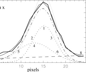
Figure 9: Example of an observed $x$-axis light profile (thick solid-line) and its corresponding best fit (thin solid-line). The dotted-lines correspond to the two gaussian components, being the dot-dashed-line the sum of these two components. The underlying emission (background) is represented by the dashed-line. The approximate positions for the 8 points used for defining the initial set of parameters are also shown. The spatial scale of the image was 0$\aas@@fstack{\prime\prime}$333 pixel^-1.

Due to the large number of star-forming regions in Mrk~86 and the intense and variable underlying emission we developed a program that allowed us to substract this underlying emission and the occasional contamination from neighbor star-forming regions. Then, on the underlying emission subtracted image, we determined the most reliable apertures, sizes, and integrated fluxes for all these regions. This program was written in fortran77 programming language and it was called COBRA (see http://www.ucm.es/info/Astrof/cobra/).

COBRA uses different graphic output devices, including xwindows and Postscript, and makes use of the AMOEBA (Press et al. press (1986)), PGPLOT, FITSIO and BUTTON (Cardiel et al. reduceme (1998); see also Cardiel cardiel99 (1999)) subroutines.

In this Appendix we will describe the procedure followed to estimate the underlying emission and the criteria used to determine the sizes and fluxes of the star-forming regions and stellar clusters in Mrk~86 using the program COBRA.

8.1 Light profiles fitting

First, (1) a image section including the region of interest is selected interactively (see the original images in Fig. 10). The size of this section necessarily depends on the spatial scale of the change in the underlying emission and the proximity of neighbor regions. This section must be chosen in such a way that the background emission (underlying and neighbor regions emission) can be reproduced by a line in the $x$ and $y$ light profiles. Thus, when several relative maxima are placed too close to match this criterion they were studied as a single region.

After cropping the image section selected, (2) the position of the maximum of the region of interest is marked interactively. Then, the light profile along the $x$ axis at this position is fitted.

In order to perform this fit three different components are used, a line that reproduced the underlying and neighbor regions contamination and two gaussians that allowed to reproduce the light profile of the region of interest. In principle, any smooth, monotonic light profile can be approximated by a serie of Gaussians (somewhat analogous to the Fourier series), not only the PSF of an image, but also the light profiles of remote stellar clusters or galactic cores (see Bendinelli et al. bendinelli (1990)). Two gaussians are employed in order to reproduce the light profile of these regions because the use of a larger number of components led in some cases to solutions with no physical meaning.

Then, the best fit for the initial light profile using the minimization subroutine AMOEBA is obtained. The AMOEBA subroutine needs an initial set of solutions which can be defined by the 8 parameters of the function to minimize (3 for each gaussian and 2 for the line). These parameters were introduced interactively marking the approximate position of the center and FWHM for each gaussian and two extreme values in the profile for the line. In Fig. 9 we show an example of the positions of the points used to define the set of initial parameters for the fit. Points 1,2,3 and 4,5,6 led to the initial parameters for the two gaussians and points 7,8 for the line. Using this set of parameters, (3) the best-fitting light profile is obtained (see Fig. 9).

Then, from the output of this fit and introducing the new positions of the two gaussian maxima, (4) all the $x$ axis profiles are fitted starting from those profiles adjacent to the initial one. The need of using previous results for the subsequent fits constitutes the main reason for starting this fitting procedure at the maximum of the emission region.

Next, (5) the same fitting procedure is applied to the $y$ axis profiles. Finally, after the profiles have been fitted in both axis, the underlying emission images reconstructed are averaged and subtracted from the original input image (see several examples in Fig. 10). This background-free image is then used to determine the centers, apertures, sizes and integrated fluxes of the different regions.

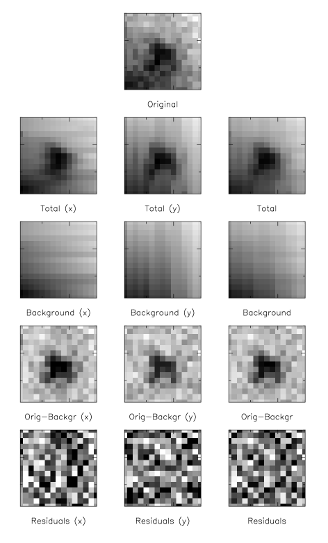
Figure 10: Original, total (reconstructed), background, original minus background model and residuals images in both axis and the average as obtained for the region #6 in the $R$-band. The cuts in the original, total and background images are the same and equal to the maximum and minimum value in the original image. The cuts in the residuals images correspond to plus/minus one tenth the difference between the maximum and minimum in the background averaged image. The residuals images were obtained as the original image minus the total (reconstructed) image.

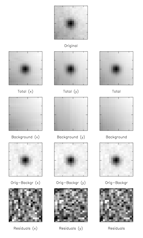
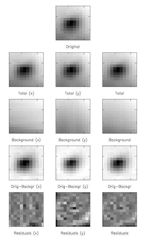
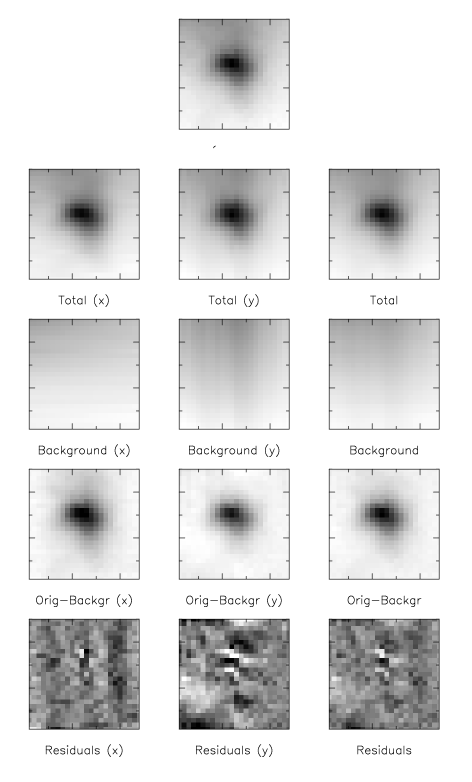
Figure 10: (cont.) Original, total (reconstructed), background, original minus background model and residuals images in both axis and the average as obtained for the region #11 in the $R$-band. The cuts in the original, total and background images are the same and equal to the maximum and minimum value in the original image. The cuts in the residuals images correspond to plus/minus one tenth the difference between the maximum and minimum in the background averaged image. The residuals images were obtained as the original image minus the total (reconstructed) image.

Figure 10: (cont.) Original, total (reconstructed), background, original minus background model and residuals images in both axis and the average as obtained for the region #18 in the $R$-band. The cuts in the original, total and background images are the same and equal to the maximum and minimum value in the original image. The cuts in the residuals images correspond to plus/minus one tenth the difference between the maximum and minimum in the background averaged image. The residuals images were obtained as the original image minus the total (reconstructed) image.

Figure 10: (cont.) Original, total (reconstructed), background, original minus background model and residuals images in both axis and the average as obtained for the region #70 in the $R$-band. The cuts in the original, total and background images are the same and equal to the maximum and minimum value in the original image. The cuts in the residuals images correspond to plus/minus one tenth the difference between the maximum and minimum in the background averaged image. The residuals images were obtained as the original image minus the total (reconstructed) image.

8.2 Position, sizes and fluxes

The knot center is taken as the maximum of the sum of the two gaussian components. Then, computing the knot surface, $A_{\mathrm{x}}$, above different thresholds, $I_{\mathrm{x}}$, we can estimate the equivalent knot e-folding radius, $R_{\mathrm{e-folding}}$, using,

$$R_{\mathrm{e-folding}}=\sqrt{\frac{A_{\mathrm{x}}}{\pi\ln(\frac{I_{\mathrm{max}}}{I_{\mathrm{x}}})}}$$ (1)

where $I_{\mathrm{max}}$ is the knot maximum intensity. In Fig. 11 we show the change in the area $A_{\mathrm{x}}$ for different thresholds as measured in the background subtracted image of the star-forming region #18 (with 1 e-folding radius of 0$\aas@@fstack{\prime\prime}$93). The relatively small change deduced for the e-folding radius with the threshold guarantees the goodness of this size determination procedure.

Figure 11: Change in the area ($A_{\mathrm{x}}$) of the region #18 with the threshold, $I_{\mathrm{x}}$. The solid-line represents the result expected for a radius of 0$\aas@@fstack{\prime\prime}$9 at 1 e-folding. The dashed-lines correspond to 0$\aas@@fstack{\prime\prime}$8 and 1$\aas@@fstack{\prime\prime}$0 e-folding radii.

The e² and e³-folding radii are then computed as $\sqrt{2}$ and $\sqrt{3}$ times the e-folding radius. Then, the knot contours are derived at these three radii, i.e. at $I_{\mathrm{max}}$/$I_{\mathrm{x}}$=e,e²,e³. The knot total flux is computed as the total flux in the background subtracted image. In order to ensure that most of the knot flux was included we derive the knot growing-curve, finding differences not larger than 20 per cent between total and growing-curve extrapolated flux.

References

- (1) Alonso-Herrero A., Aragón-Salamanca A., Zamorano J., Rego M., 1996, MNRAS 278, 417
- (2) Aragón-Salamanca A., Ellis R.S., Couch W.J., Carter D., 1993, MNRAS 262, 764
- (3) Arp H., 1966, Atlas of Peculiar Galaxies. California Institute of Technology, Pasadena
- (4) Bendinelli O., Parmeggiani G., Zavatti F., Djorgovski S., 1990, AJ 99, 774
- (5) Bonatto C., Bica E., Pastoriza M.G., Alloin D., 1999, A&A 343, 100
- (6) Bottinelli L., Gouguenheim L., Fouqué P., Paturel G., 1990, A&AS 82, 391
- (7) Brocklehurst M., 1971, MNRAS 153, 471
- (8) Burkert A., 1989, Ph.D. Thesis, Munich
- (9) Campbell A.W., Terlevich R., 1984, MNRAS 211, 15
- (10) Cardiel N., 1999, Ph.D. Thesis, Universidad Complutense de Madrid
- (11) Cardiel N., Gorgas J., Cenarro J., González J.J., 1998, A&AS 127, 597
- (12) Cassatella A., Barbero J., Benvenuti P., 1985, A&A 144, 335
- (13) Doublier V., 1998, Ph.D. Thesis, Marsella
- (14) Drinkwater M., Hardy E., 1991, AJ 101, 94
- (15) Dultzin-Hacyan D., Masegosa J., Moles M., 1990, A&A 238, 28
- (16) Elias J.H., Frogel J.A., Matthews K., Neugebauer G., 1982, AJ 87, 1029
- (17) Elson R.A.W., Fall S.M., 1985, PASP 97, 692
- (18) Fanelli M.N., O’Conell R.W., Thuan T.X., 1988, ApJ 334, 665
- (19) Fernie J.D., 1983, PASP 95, 782
- (20) Fuentes-Masip O., 1997, Ph.D. Thesis, La Laguna
- (21) Fukuguita M., Shimasaku K., Ichikawa T., 1995, PASP 107, 945
- (22) Garcí-Dabó C.E., Gallego J., 1999, Ap&SS 263, 1-4
- (23) Gil de Paz A., Zamorano J., Gallego J., 1999, MNRAS 306, 975 (GZG)
- (24) Gil de Paz A., Zamorano J., Gallego J., 2000a, A&A (Paper II)
- (25) Gil de Paz A., Aragón-Salamanca A., Gallego J., et al., 2000b, MNRAS 316, 357
- (26) Giovanelli R., Haynes M.P., Herter T., et al., 1997, AJ 113, 53
- (27) Hoffman G.L., Salpeter E.E., Helou G., 1990, in the proceedings of the Edwin Hubble Centennial Symposium, 67
- (28) Kennicutt R.C., Edgar B.K., Hodge P.W., 1989, ApJ 337, 761
- (29) Kent S.M., 1985, PASP 97, 165
- (30) Klein U., Wielebinski R., Thuan T.X., 1984, A&A 141, 241
- (31) Klein U., Weiland H., Brinks E., 1991, A&A 246, 323
- (32) Kunth D., Sargent W.L.W., 1986, ApJ 300, 496
- (33) Kunth D., Maurogordato S., Vigroux L., 1988, A&A 204, 10
- (34) Landolt A.U., 1973, AJ 78, 959
- (35) Loose H.-H., Thuan T.X., 1985, The Morphology and Structure of BCDGs from CCD Observations, in: Kunth, D., Thuan, T.X., and Van, J.T.T.(eds.) Star-Forming Dwarf Galaxies. Editions Frontières.
- (36) Markarian B.E., 1969, Astrofizika 5, 443
- (37) Marlowe A.T., Heckman T.M., Wyse R.F.G., Schommer R., 1995, ApJ 438, 563
- (38) Martin C. L., 1998, ApJ 506, 222
- (39) Mazzarella J.M., Boroson T., 1993, ApJS 85, 27
- (40) Norton S., Salzer J.J., 1997, BAAS 190
- (41) Osterbrock D.E., 1989, Astrophysics of Gaseous Nebulae and Active Galactic Nuclei. University Science Books, Mill Valley, California.
- (42) Papaderos P., Loose H.-H., Thuan T.X., Fricke K.J., 1996a, A&AS 120, 207
- (43) Papaderos P., Loose H.-H., Fricke K.J., Thuan T.X., 1996b, A&A 314,59
- (44) Petrosian A.R., Boulesteix J., Comte G., Kunth D., LeCoarer E., 1997, A&A 318, 390
- (45) Press W. H., Flannery B.P., Teukolsky S.A., Vetterling W.T., 1986, Numerical Recipes, Cambridge University Press
- (46) Rood H.J., Dickel J.R., 1976, ApJ 205, 346
- (47) Sage L.J., Salzer J.J., Loose H.-H., Henkel C., 1992, A&A 265, 19
- (48) Scalo J.M., 1986, Fund. Cosmic Phys. 11, 1
- (49) Searle L., Sargent W.L.W., 1972, ApJ 173, 25
- (50) Searle L., Sargent W.L.W., Bagnuolo W.G., 1973, ApJ 179, 427
- (51) Shapley H., Ames A., 1932, Ann. Harvard College Obs. 88, No. 2
- (52) Sharina M.E., Karachentsev I.D., Tikhonov N.A., 1999, Astronomy Letters 25, 322
- (53) Silk J., Wyse R.F.G., Shields G.A., 1987, ApJ 322, L59
- (54) Thronson Jr. H.A., Telesco C.M., 1986, ApJ 311, 98
- (55) Thuan T.X., 1983, ApJ 268, 667
- (56) Thuan T.X., 1991, Observations and Models of Blue Compact Dwarf Galaxies, in: Leitherer C., Walborn R.N., Heckman T.M., Norman C.A. (eds.) Massive Stars in Starbursts, Cambridge University Press, p.183.
- (57) Thuan T.X., Martin G.E., 1981, ApJ 247, 823
- (58) Trager S.C., Worthey G., Faber S.M., Burstein D., González J.J., 1998, ApJS 116, 1
- (59) Verter F., 1985, ApJS 57, 261
- (60) Wainscoat R.J., Cowie L.L., 1992, AJ 103, 332