Uncertainties on Clusters of Galaxies Distances.
Abstract
We investigate in this paper the error on the cluster redshift estimate as a function of: (1) the number of galaxy structures along the line of sight; (2) the morphology of the clusters (regular/substructures); (3) the nature of the observed galaxies (cD/normal galaxies); (4) the number of observed galaxies; and (5) the distance of the clusters. We find that if we use cD galaxies we have errors of less than 2% (at the 1- level) for the cluster distances except when the clusters are very complex. In those cases when we use five redshift measurements along the cluster lines of sight to compute the mean redshift, the mean redshift estimate error is less than 5 for the clusters closer than z=0.30. The same error of 5% for clusters in z=[0.30;0.60] requires about 12 redshifts measurements.
Methods: numerical ; Methods: statistical ; Galaxies: clusters: general
1 Introduction
Large surveys of clusters of galaxies are commonly used in modern observational cosmology both for optical (e.g. ENACS: Katgert et al. 1996, CNOC: Carlberg et al. 1996) and X-ray studies (e.g. Ebeling et al. 1998, Rosati et al. 1998, Vikhlinin et al. 1998, Romer et al. 2000). Only the mean redshift of the clusters is necessary for example for constraining cosmological models using the N/z relation (Oukbir Blanchard 1997), i.e. the variation of the cluster abundance as a function of redshift and mass. Since masses of these clusters can be measured from X-ray data, thus spectroscopy is only necessary to compute the mean redshift. For very large (typically more than 100 clusters) and deep surveys, however, it is difficult to measure a large number of redshifts for each cluster due to observing time constraints. But, too low a number of redshifts can induce errors for the mean redshift. We propose in this work to quantify these errors by using simulations. The purpose of this paper is to provide guidelines for estimating statistical errors on the distance of clusters of galaxies in existing catalogs as a function of the galaxies sampled (number of redshifts per line of sight and nature of the galaxies) and of the distances and characteristics of these clusters. Estimates based only on a small number of redshifts and a limited number of cases can be found in Holden et al. (2000).
The first part of the article describes the method and the sample. The second part gives the results of the simulations. The third part discusses these results.
We used H0=100 km.s-1.Mpc-1 and q0=0.05.
2 General methodology and Sample.
We have tested the influence on the mean redshift uncertainty of: (1) the number of galaxy structures along the line of sight; (2) the morphology of the clusters (regular/substructures); (3) the nature of the observed galaxies (cD/normal galaxies); (4) the number of observed galaxies; and (5) the distance of the clusters.
These clusters were selected from the ENACS database (Katgert et al. 1996), from a literature compilation by A. Biviano (described for example in Adami et al. 1998), and from the public CNOC database (Carlberg et al. 1996). We only selected the very well sampled clusters, i.e. those with a sufficient number of redshifts to allow us to assume safely that the redshift measurements provided the true value of the mean cluster redshift. We then resampled each of these clusters with galaxies before re-computing the mean redshift to estimate the error for this redshift. The method we used to compute the mean redshift after the resampling with galaxies is as follows: we used the same analysis methods as for the ENACS lines of sight (Katgert et al. 1996). We excluded the galaxies classified as field objects (see below) and we used a Biweight estimator (Beers et al. 1990) of the mean for the cluster galaxies. Briefly, field galaxies were discriminated by searching for velocity gaps of more than 1000 km.s-1 in the redshift distributions of the galaxies sorted by increasing redshift. If two galaxies were separated by more than 1000 km.s-1, they were assumed to belong to different structures. The method is explained in detail in Katgert et al. (1996), but we note that the choice of a value of 1000 km.s-1 for the gap has no significant influence on the structure membership determination (see Adami et al. 1998): a value between 600 and 1200 km.s-1 gives similar results.
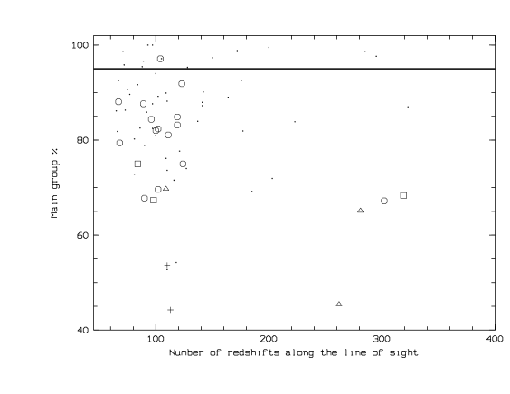
In order to remove possible interloper clusters (with too small a number of redshifts) from the sample, we selected only the lines of sight with more than 50 redshifts in the main groups (the “clusters” hereafter). We also discarded the lines of sight with too high a contamination level in a first step: we rejected the lines of sight with more than two structures sampled with more than 20 redshifts. This limitation corresponds approximatively to the separation between the massive and minor groups in the ENACS sample. These lines of sight are considered in section 3.3. At this step, there were 73 lines of sight in the sample. As we used a literature compilation, selection effects are sometimes significant. For example, galaxies along a few lines of sight in the sample were observed by using a color-magnitude selection of the targets (Mazure et al. 1988) or only the cluster galaxy redshifts were given in the literature. This potentially induced a bias toward the cluster galaxies. In order to limit this problem, we discarded all the lines of sight with more than 95% of the galaxies inside the main cluster (cf. Fig. 1) because these lines of sight were very likely to be biased toward the cluster galaxies. This value of 95% is based on our analysis of the ENACS results (Katgert et al. 1996). In this survey there was no selection of galaxies with a color-magnitude relation. All the redshifts measured along the lines of sight were provided. We found that these ENACS lines did not have more than 95% of the galaxies within a single structure.
In total, after all the rejections, we used a sample of 58 lines of sight (Table 1). We split this sample of 58 clusters in five different redshift bins in order to compute the redshift estimate precision as a function of the cluster distance (and of the number of sampling galaxies). The first bin (z=[0; 0.07]) contains 37 clusters, the second bin (z=[0.07; 0.13]) contains 14 clusters, the third and the fourth bins (z=[0.13,0.30] and z=[0.30,0.45]) contain 3 clusters and the last bin (z=[0.45,0.60]) contains 2 clusters. We note that the fourth and the last bins mainly used CNOC data (Carlberg et al. 1996).
3 The results
3.1 Lines of sight with only one dominant structure
We resampled all the 58 lines of sight (i.e. with only one dominant structure) with galaxies, with n=[5;47] (the method we used to compute the mean redshift is not effective for a sampling rate of less than 5 galaxies). In order to have the same statistical significance for each of the five redshift bins (they do not have the same number of clusters), we made about 5000 realizations (bootstrap technique with 5000 resampling) for a given (number of selected redshifts along the line of sight) and for a given cluster redshift range. This means that we made 135 different resamplings for each line of sight and each in the first redshift bin (37 clusters 135 simulations 5000 simulations), 357 different resamplings for each line of sight and each in the second redshift bin, 1667 different resamplings for each line of sight and each in the third and fourth redshift bins, and 2500 different resamplings for each line of sight and each in the fifth redshift bin.
| name | bin | galaxies | cluster galaxies | cz | distance (kpc) | vel. difference (km.s-1) | substructures |
|---|---|---|---|---|---|---|---|
| A85 | 1 | 185 | 128 | 16384 | S | ||
| A119 | 1 | 142 | 128 | 12958 | 15 | 63 | R |
| A168 | 1 | 109 | 83 | 13216 | 106 | 51 | S |
| A193 | 1 | 65 | 56 | 14285 | 22 | 125 | R |
| A400 | 1 | 109 | 98 | 6952 | 4 | 87 | |
| A496 | 1 | 164 | 146 | 9768 | 18 | 25 | R |
| A754 | 1 | 100 | 94 | 16635 | 493 | 110 | R |
| A978 | 1 | 73 | 63 | 16689 | S | ||
| A1060 | 1 | 177 | 145 | 4000 | 19 | 54 | S |
| A1185 | 1 | 77 | 69 | 9704 | 92 | 1113 | |
| A1631 | 1 | 90 | 71 | 14243 | 354 | 283 | R |
| A1644 | 1 | 102 | 91 | 14504 | 33 | 55 | S |
| A1795 | 1 | 97 | 85 | 19065 | 31 | 14 | R |
| A1983 | 1 | 100 | 81 | 13589 | 1102 | 274 | S |
| A2040 | 1 | 66 | 54 | 13976 | 24 | 133 | R |
| A2052 | 1 | 97 | 80 | 10636 | 8 | 150 | S |
| A2107 | 1 | 75 | 68 | 12474 | 7 | 265 | S |
| A2124 | 1 | 67 | 62 | 19589 | R | ||
| A2717 | 1 | 81 | 59 | 14408 | R | ||
| A2734 | 1 | 116 | 83 | 18121 | R | ||
| A2877 | 1 | 110 | 97 | 7037 | 23 | 7 | |
| A3122 | 1 | 121 | 94 | 19173 | S | ||
| A3128 | 1 | 223 | 187 | 17927 | 279 | 412 | S |
| A3158 | 1 | 141 | 123 | 17606 | 43 | 213 | R |
| A3223 | 1 | 110 | 81 | 18035 | 79 | 1158 | S |
| A3341 | 1 | 118 | 64 | 11377 | S | ||
| A3354 | 1 | 110 | 58 | 17604 | S | ||
| A3376 | 1 | 84 | 77 | 14063 | |||
| A3391 | 1 | 81 | 65 | 16302 | |||
| A3395 | 1 | 203 | 146 | 15283 | |||
| A3558 | 1 | 323 | 281 | 14612 | 5 | 270 | R |
| A3651 | 1 | 92 | 79 | 17817 | S | ||
| A3667 | 1 | 176 | 163 | 16557 | 1 | 73 | R |
| A3716 | 1 | 137 | 115 | 13792 | |||
| A3744 | 1 | 86 | 71 | 11169 | S | ||
| A3809 | 1 | 127 | 94 | 18430 | R | ||
| A401 | 2 | 123 | 113 | 21868 | 92 | 591 | R |
| A514 | 2 | 111 | 90 | 21589 | 778 | 892 | R |
| A1809 | 2 | 67 | 59 | 23985 | 13 | 69 | R |
| A2029 | 2 | 89 | 78 | 23124 | 9 | 458 | |
| A2142 | 2 | 119 | 101 | 27107 | |||
| A2670 | 2 | 302 | 203 | 22494 | 15 | 447 | S |
| A2721 | 2 | 100 | 82 | 34039 | |||
| A3094 | 2 | 102 | 71 | 20004 | S | ||
| A3112 | 2 | 124 | 93 | 22460 | 4 | 203 | R |
| A3695 | 2 | 96 | 81 | 26678 | S | ||
| A3705 | 2 | 68 | 54 | 26647 | S | ||
| A3806 | 2 | 119 | 99 | 22772 | S | ||
| A3822 | 2 | 102 | 84 | 22536 | S | ||
| A3825 | 2 | 90 | 61 | 22327 | 386 | 116 | R |
| A1146 | 3 | 84 | 63 | 43207 | |||
| A2390 | 3 | 319 | 218 | 68370 | |||
| A3888 | 3 | 98 | 66 | 45434 | |||
| MS1008-12 | 4 | 109 | 76 | 91860 | 87 | 63 | R |
| MS1358+62 | 4 | 281 | 183 | 98700 | 202 | 780 | S |
| MS1621+26 | 4 | 262 | 119 | 128220 | S | ||
| MS0015+16 | 5 | 110 | 59 | 162270 | R | ||
| MS0451-03 | 5 | 113 | 50 | 158790 | R |
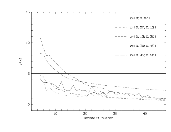
For each of the 5000 realizations we computed the difference between the true value of the cluster redshift and the estimated value of this redshift. We finally computed the dispersion of the 5000 percentage differences. The mean values of these difference percentages were always consistent with an error of 0% and in the range . We focus here on the variation of the dispersion of these 5000 differences as a function (the number of selected redshifts along the line of sight). These variations are given in Fig. 2 for the five different cluster redshift bins. The 1- error is always less than 5% for the clusters at z0.30, whatever the number of redshifts (greater than 5) we use along the line of sight to compute the mean distances of the clusters. These errors become greater than 5% (but are still lower than 10%) for the clusters more distant than z=0.30 when we use less than 13 galaxies along the lines of sight to compute the mean redshifts of the clusters.
3.2 Influence of the nature of the clusters: regular vs substructured clusters.
The dynamical state of the clusters is also important for the redshift estimate: regular or with more perturbed history. When the clusters have a very complex velocity structure we need to know if the statistical approach of using a larger number of fainter galaxies will succeed.
We have chosen to repeat the analysis of Section 3.1. This time we used a discrimination between the regular and the irregular clusters. We used the work of Bird (1994), Bird Beers (1993) and Solanes et al. (1999) to produce a classification for the Abell clusters in our sample. These authors have performed substructure tests with a subsample of the clusters in Table 1. We classified a cluster of Table 1 as regular only if no one of the tests provided by these authors gave evidence of substructures at the 10 level. For the CNOC clusters, we plotted galaxy isodensity contours and we selected as regular the clusters providing regular contours. We assumed that no substructures in a cluster was an indication of a quiescent history. The same kind of classification could possibly be achieved in the future using X-ray data. However, for most of the clusters in our sample, the only X-ray images available have too low a spatial resolution or too weak a signal to allow us to resolve substructures for the distant clusters.
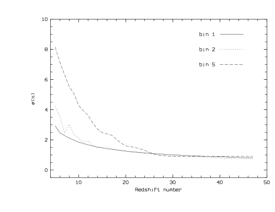
We have separated the clusters of the sample with substructure information into 3 redshift bins: the bins 1, 2 and 5 of Section 3.1 (the bins 3 and 4 do not provide alone robust estimates). We plot on Fig. 3 the variation of the redshift error percentage as a function of the number of measured galaxies used to compute the mean distance of the cluster for the regular clusters. This is directly comparable with the percentages given in Fig. 2. We see that the error percentages are slightly lower when we use the regular clusters compared to the whole sample (regular + substructured + unknown). The difference is close to 1 or 2 percent. This means that the clusters with substructures do not produce very significantly higher errors in the mean redshift estimate. The approach of Section 3.1 is, therefore, not very sensitive to the nature of the clusters.
3.3 Lines of sight with more than one dominant structure
We only use here the clusters satisfying the conditions of Sect. 3.1, but with at least one group with more than 20 galaxies in addition to the main structure. These clusters are A151 (z=0.052, 3 groups with more than 20 gal.), A1656 (z=0.024, 3 groups with more than 20 gal.), A2390 (z=0.23, 2 groups with more than 20 gal.), A2634 (z=0.030, 2 groups with more than 20 gal.), A4038 (z=0.029, 5 groups with more than 20 gal.) and MS1512+36 (z=0.37, 3 groups with more than 20 gal.). The results of the simulations show a higher 1- error in percentage, as expected, but the difference is not very significant. First, we have no difference when we use more than 10 redshifts, whatever the distance of the cluster is. When we used less than 10 redshifts, we add about 2 to the values of Fig. 2. We have an unchanged number of redshifts required to have an error smaller than 5 for z0.3. For z0.3, we now need more than 8 or 9 redshifts measurements (instead of 5). We also note that such superpositions are not very likely. They represent only 10 of the total sample we used in this study. We will, therefore, refer only to the Fig. 2 results.
3.4 Influence of the nature of the galaxies: using the cD velocities.
The three previous sub-sections deal with normal galaxies. However, an important question with fundamental implications is to know if the first ranked galaxy (assumed to be the central Dominant galaxy hereafter) is a good measure of the cluster redshift. This kind of galaxy is, in a simple picture, at the bottom of the cluster potential, at the spatial center of the cluster and, therefore, at a redshift very close to the mean cluster redshift. In theory, this allows the cluster redshift measurement to be made with only one galaxy (e.g. Gunn et al. 1986, Hill Oegerle 1998). However, when the cluster history is complex (mergings), the cD galaxies can be sometimes classified as (see e.g. Zabludoff et al. 1993 and references therein), i.e. cD galaxies with a significant velocity difference compared to the mean cluster velocity. Moreover, those can be shifted compared to the cluster center (e.g. Peres et al. 1998). In this case, the use of the cD alone can fail in measuring accurately the cluster mean redshift.
In order to investigate this point, we have used the clusters of our real sample using the first ranked galaxies with a measured redshift. Moreover, to separate the normal cD’s and the speeding cD’s, we used only the clusters with an X-ray center (see Tab. 1). The peak emission of the X-ray gas is assumed to be the real center. The distance between the cD and the X-ray center is used as an indication of the nature of the cD galaxies. When the cD galaxy is located at less than 50 kpc in projected distance from the cluster center (the X-ray center), the difference between the cluster mean velocity and the cD velocity is (0.150.12) (with the biweight velocity dispersion of the cluster). For the cD’s at more than 50 kpc, the difference is (0.530.47) . Despite the large uncertainties, it seems clear that when the cD’s are far from the X-ray center, they provide a less reliable estimate of the mean cluster velocity: for a typical cluster with a velocity dispersion of 1000 km.s-1, the mean difference is 550 km.s-1 (150 km.s-1 when X-ray center and cD position match).
Besides testing the cD derived redshift as a function of the distance from the cluster center, we also tested the cD versus the mean redshift (as identify the true cD can be more difficult with increasing redshift). In order to have enough clusters with an X-ray center in each bin, we could only separate the sample into two bins: redshifts lower and higher than 0.06. For the nearby clusters and the cD galaxies close to the center, the error on the cluster mean redshift estimate is (0.140.11). For the nearby clusters and the cD galaxies far from the center, the error is (0.390.29). For the more distant clusters and the cD galaxies close to the center, the difference is (0.190.16) . Finally, for the more distant clusters and the cD galaxies far from the center, the difference is (0.680.60) . According to the uncertainties, the differences are not very significant but still very suggestive. Whatever the cluster redshift (nearby or more distant), the cD galaxies close to the center are better estimators of the mean cluster velocity compared to the cD galaxies far from the center. However, this trend tends to become stronger at higher redshifts, perhaps due to the fact that we are dealing with younger structures, therefore at earlier formation stage and smaller than present day clusters.
The conclusion of this section is that the cD galaxies are good estimators of the cluster velocities when they are not speeding cD galaxies. Given in the same units as in the previous sections, the redshift error is lower than 1 when we use the cD galaxy redshift as the cluster redshift.
When we deal with disturbed clusters and speeding cD galaxies, the error is larger but often acceptable: for example for clusters at z=0.05 and with a velocity dispersion of 1000 km.s-1, the error on the mean redshift estimate is 32 . However, in a few cases, this error can be close to 10 (at the 3- level). Moreover, for the very distant cluster, it is not trivial to find which galaxy is the dominant one due to foreground galaxies. In these cases, the cD approach fails to measure the mean distance of the clusters.
4 Summary
We have used a sample of 58 rich clusters of galaxies (from z=0 to z=0.60) in order to investigate the error on the cluster redshift estimate as a function of the distance of the cluster, of the number of measured redshifts along the line of sight, of the nature of the galaxies (cD galaxies or normal galaxies) and of the nature of the clusters (regular/substructures).
The mean redshift of the clusters are used, for example, to compute the absolute magnitudes of the galaxies in a given cluster from the observed apparent magnitudes (luminosity function studies, e.g. Lumsden et al. 1997, Valotto et al. 1997, Rauzy et al. 1998) or to measure the X-ray luminosity of this cluster (e.g. Romer et al. 2000) from the observed X-ray flux. If we require an error in the optical magnitude of a cluster galaxy of less than 0.25 magnitude or of less than 10% on a cluster X-ray luminosity, we need to measure the mean redshift of this cluster with an accuracy of less than 5%. For nearby clusters (z0.30), if we use our method to compute the mean redshift (discrimination of field galaxies with a gap analysis and Biweight estimators of the mean: Beers et al. 1990), the error on the redshift estimate is better than 5% even with only 5 redshift measurements along the line of sight.
If we now consider more distant clusters (z in the [0.30;0.60] range), we have an error of less than 5% if we measure more than 12 redshifts along the line of sight. With only 5 redshifts, the error on an optical magnitude can be (at the 67% level) 0.5 mag and that on an X-ray luminosity will be 20%. These estimates use galaxy redshifts distributed in a region of about 4 h-2Mpc2 (the typical size covered for each cluster in clusters of galaxy surveys such as ENACS: Katgert et al. 1996) around the cluster centers and magnitude without selection criteria. This means that the errors we plotted in Fig. 2 probably would decrease with a more concentrated survey around the cluster centers (but we have not tested this point in this article).
We show that it is slightly easier to measure an accurate mean redshift for the regular clusters (with quiescent history and, therefore, with symmetric potential well) using the approach of Section 3.1 (measuring a few dozens of redshifts). This method does not provide, however, significantly worse results for the substructured clusters (with more perturbed an history).
Finally, we showed that for the regular clusters, the measure of the cD galaxy redshift is a good way to measure accurately the mean redshift of the parent-cluster. Sometimes, however, this approach fails (for the substructured clusters or very distant clusters where the cD nature of a given galaxy is not straightforward to define). This approach should be replaced with a multi-redshift measure. The 5 error level is reached with 5 redshift measurements for the cluster closer than z=0.30 and with about 12 redshift measurements for the more distant clusters (z0.60).
Acknowledgements.
CA thanks the Dearborn Obs. staff for their hospitality during his postdoctoral fellowship. CA and MPU thank the referees for useful and constructive comments, Florence Durret for a careful reading of the manuscript and Andrea Biviano for his compilation. CA thanks the LAM for support.References
- (1) Adami C., Biviano A., Mazure A., 1998, AA 331, 439
- (2) Beers T.C., Flynn K., Gebhardt K., 1990, AJ 100, 32
- (3) Bird C.M., 1994, AJ 107, 1637
- (4) Bird C.M., Beers T., 1993, AJ 105, 1596
- (5) Carlberg R.G., Yee H.K.C., Ellingson E., et al., 1996, ApJ 462, 32
- (6) Ebeling H., Edge A.C., Bohringer H., et al., 1998, MNRAS 301, 881
- (7) Gunn J.E., Hoessel J.G., Oke J.B., 1986, ApJ 306, 30
- (8) Hill J.M., Oegerle W.R., 1998, AJ 116, 1529
- (9) Holden B.P., Nichol R.C., Romer A.K., et al., 2000, ApJ in press, astro-ph: 9907429
- (10) Katgert P., Mazure A., Perea J., et al., 1996, AA 310, 8
- (11) Lumsden S.L., Collins M.A., Nichol R.C., Eke V.R., Guzzo L., 1997, MNRAS 290, 119
- (12) Mazure A., Proust D., Mathez G., Mellier Y., 1988, AAS 76, 339
- (13) Oukbir J., Blanchard A., 1997, AA 317, 365
- (14) Peres C.B., Fabian A.C., Edge A.C., et al., 1998, MNRAS 298, 416
- (15) Rauzy S., Adami C., Mazure A., 1998, AA 337, 31
- (16) Romer A.K., Nichol R.C., Holden B.P., et al., ApJ in press
- (17) Rosati O., Della Ceca R., Norman C., Giacconi R., 1998, ApJ 492, 21
- (18) Solanes J.M., Salvador-Sole E., Gonzales-Casado G., 1999, AA 343, 733
- (19) Valotto C.A., Nicotra M.A., Muriel H., Lambas D.G., 1997, ApJ 479, 90
- (20) Vikhlinin A., McNamara B.R., Forman W., et al., 1998, ApJ 502, 558
- (21) Zabludoff A.I., Geller M.J., Huchra J.P., Vogeley M.S., 1993, AJ 106, 1273