Inter-scale correlations as measures of CMB Gaussianity

Abstract

A description of CMB temperature fluctuations beyond the power spectrum is important for verifying models of structure formation, especially in view of forthcoming high-resolution observations. We argue that higher-order statistics of inter-scale correlations, because of their low cosmic variance, may be effective in detecting non-Gaussian features in the CMB. Inter-scale correlations are generically produced in defect-based models of structure formation. We analytically study properties of general higher-order cumulants of Fourier components of homogeneous random fields and design a new set of statistics suitable for small-scale data analysis. Using simulated non-Gaussian fields, we investigate the performance of the proposed statistics in presence of a Gaussian background and pixel noise, using the bispectrum as the underlying cumulant. Our numerical results suggest that detection of non-Gaussian features by our method is reliable if the power spectrum of the non-Gaussian components dominates that of the Gaussian background and noise within at least a certain range of accessible scales.

98.70.V;98.80.C

I Introduction

The fluctuations in the cosmic microwave background (CMB) radiation first reliably measured by the COBE [1] are one of today’s most cosmologically important measurements (see [2] for a recent review). The future satellite missions MAP [3] and PLANCK [4] are expected to provide high-resolution, low-noise CMB data that will strongly constrain current theories of structure formation. One of the key differences between the competing theories is an approximately Gaussian distribution of density fluctuations produced in most inflationary theories versus the generically non-Gaussian inhomogeneities in scenarios based on topological defects. A precise statistical analysis of the CMB fluctuations is needed to distinguish non-Gaussian signatures of cosmic defects [5] and small deviations from Gaussianity in inflationary universe due to generic effects such as a non-linear evolution [6, 7], gravitational lensing [8], and higher-order couplings during recombination [9]. The power spectrum, which is the statistic easiest both to predict theoretically and to extract from data, is by definition insensitive to non-Gaussian correlations. For this reason, and especially in view of forthcoming observations, detection of non-Gaussian features in the CMB is an important task.

Since all theories give only statistical predictions of the CMB, one’s conclusions from a single observation of the microwave sky are by necessity probabilistic. Many criteria of Gaussianity have been proposed in the literature and applied to the available data, mostly yielding results consistent with the Gaussian hypothesis [10]. Although some claims of finding a non-Gaussian signal in COBE have been advanced recently [11, 12, 13, 14], not all of them are equally persuasive and some have been ascribed to data contamination and noise in Refs. [15, 16]. Apart from these problems, the usefulness of any CMB statistic is fundamentally limited by cosmic variance. Therefore we would like to look for statistical descriptors of non-Gaussian signal that have a naturally low variance.

Cosmic variance manifests itself differently in real space and in the Fourier space where the CMB temperature fluctuations are usually decomposed into modes $a_{lm}$ using the spherical harmonic expansion

$$\frac{\Delta T}{T}\left(\theta,\phi\right)=\sum_{l,m}a_{lm}Y_{lm}\left(\theta,\phi\right).$$ (1)

The power spectrum estimator

$$C_{l}=\frac{1}{2l+1}\sum_{m=-l}^{l}\left|a_{lm}\right|^{2}$$ (2)

is increasingly more precise at smaller angular scales (higher $l$). In other words, the cosmic variance in the Fourier space is shifted away from small scales toward large scales. One would therefore expect any statistics of Fourier modes at very small scales to be relatively free of cosmic variance. On the other hand, real space data is correlated and estimators based on correlations of $\Delta T\left(\theta,\phi\right)$ are equally affected by cosmic variance throughout all angular scales. (The recently introduced wavelet-based statistics [17, 13] can be regarded as occupying the middle ground between the real and the Fourier space descriptors. See also [18] for an example of a low-variance real-space statistic which is however strongly power-spectrum dependent.)

This motivates us to consider small-scale Fourier modes in hopes of obtaining a sensitive statistic. Previous research [19] suggests that individual Fourier modes are likely to be nearly Gaussian distributed because of the central limit theorem. Therefore we intend to investigate inter-scale correlations in Fourier space for the role of non-Gaussian indicators. A non-Gaussian signal may manifest itself as a correlation between Fourier modes $a_{lm}$ of different scales $l$; this extra correlation must be of third order or higher because homogeneity requires $\left\langle a_{lm}a^{*}_{l^{\prime}m^{\prime}}\right\rangle\propto\delta_{ll^{\prime}}\delta_{mm^{\prime}}$. The third-order correlator of the Fourier modes, called the “bispectrum”, has been extensively studied in the literature [20, 21, 22, 23, 6] and recently applied to the COBE data [11, 14]. It was shown that the bispectrum carries signatures from cosmic defects, as well as from non-linearities of evolution in inflationary models. Defects generically produce non-Gaussian features also in higher-order correlations, as we shall show.

We would like to reformulate the problem of finding the cross-correlation between some chosen scales $l$ and $l^{\prime}$ as a Gaussianity test on a suitable distribution. Consider for simplicity a random field in flat (two-dimensional) space, decomposed into Fourier modes $a_{{\mathbf{k}}}$. We may regard the set of mode values $a_{{\mathbf{k}}},\,a_{{\mathbf{k}}^{\prime}}$ at the scales $\left|{\mathbf{k}}\right|$, $\left|{\mathbf{k}}^{\prime}\right|$ as a sample of a two-variable distribution $\left\{a,a^{\prime}\right\}$ and proceed to test that distribution for Gaussianity. A general way of testing a distribution for Gaussianity is by using cumulants (see e.g. [24]). In our case we need to employ suitable multi-variable cumulants, such as a third-order cumulant

$$\chi\left(k_{1},k^{\prime}_{1},k_{2}\right)=\left\langle a_{{\mathbf{k}}_{1}}a_{{\mathbf{k}}^{\prime}_{1}}a_{{\mathbf{k}}_{2}}\right\rangle,$$ (3)

with $\left|{\mathbf{k}}_{1}\right|=\left|{\mathbf{k}}^{\prime}_{1}\right|\neq\left|{\mathbf{k}}_{2}\right|$. Such cumulants describe non-Gaussian correlations between perturbations at different scales. Since the variance of a cumulant estimator is decreased when the number of points in the sample grows, we expect the statistic to be increasingly more sensitive on smaller scales (larger $l$). We shall demonstrate for a Gaussian field that Fourier space cumulant estimators of any order $n$, which we denote $\chi\left(k_{1},...,k_{n}\right)$, at small scales (large $k_{i}$) are statistically approximately independent and themselves approximately Gaussian distributed. We also find the variances of these cumulant estimators of any order. This significantly simplifies the likelihood analysis, since the variances are theoretically known and the estimators can be normalized to have unit variances.

In other words, if the underlying CMB map were Gaussian, all quantities $\chi\left(k_{1},...,k_{n}\right)$ for all scales $k_{i}$ form (after normalization) a sample of independent realizations of a normal distribution. One could test this hypothesis by choosing an appropriate range of accessible scales $k_{i}$, combining all estimators $\chi\left(k_{1},...,k_{n}\right)$ at these scales into one sample and computing the first few cumulants $\omega_{j}$ (we take $j=1,...,5$) of that sample. If the Gaussian hypothesis holds for the original distribution, the quantities $\omega_{j}$ are in turn Gaussian distributed with known means and variances. We now propose this as a Gaussianity test for the original map. Likelihood analysis of the descriptors $\omega_{j}$ is at least as strong as a simultaneous fit of all inter-scale cumulants and is potentially more discriminating.

In this method, one is free to choose a subset of cumulants $\chi\left(k_{1},...,k_{n}\right)$ and a subset of scales $k_{i}$ at which to evaluate them. Since the statistical variance of the cumulant estimators is decreased at smaller scales (larger $k_{i}$) but grows as $n!$ with the order $n$ of the cumulants, the most promising results should come from the lowest cumulants, such as the bispectrum ($n=3$), and at smallest available scales. In this initial investigation we use only the bispectrum to build the estimators $\omega_{n}$.

To evaluate the efficiency of the method, we use several simulated non-Gaussian fields inspired by defect-based structure formation models. One of the simulated models consists a superposition of fixed temperature profiles centered on a random set of Poisson distributed points. The advantage of this model is that for any shape of the profile and for any distribution of the profile intensity and size, one can analytically obtain the full generating functional of the resulting random field, which allows (in principle) to evaluate any statistic. In particular, it is straightforward to estimate the expected inter-scale correlations of Fourier modes of this field. Another model we used is a simulated CMB map from cosmic strings [25], superimposed on Gaussian background and pixel noise. Our goal in all simulations was to find the levels of Gaussian backgrounds at which the non-Gaussian signal is still detectable with our statistic, given a certain level of noise.

The outline of the paper is as follows. In Sec. II we define the particular cumulants that describe inter-scale correlations of the Fourier modes of a random field and show how we estimate them from a single field realization. We derive the means and variances of these cumulant estimators assuming Gaussian random field, as would be needed for likelihood analysis, and show that the error bars decrease for large $l$, as expected. Details of the calculations are given in Appendices A and B. In Sec. III we describe a model non-Gaussian field made up of a random superposition of shapes, analytically determine the expected non-vanishing cumulants, and investigate the sensitivity of our criterion for that model in presence of Gaussian backgrounds. The necessary formalism is developed in Appendix C. In Sec. IV we present numerical results obtained with several simulated non-Gaussian maps using the lowest-order statistic based on the bispectrum. The method is tested on maps of point sources, random rectangles, and cosmic strings, mixed with Gaussian background and noise. We give brief conclusions about the viability of the proposed method.

II Cumulants in Fourier space

For simplicity, in this section we consider random fields on a plane; the results can be straightforwardly generalized to random fields on a sphere, such as the CMB temperature perturbation $\Delta T\left(\phi,\theta\right)/T$. From the Fourier space viewpoint, a random field $f\left(x\right)$ is a collection of random variables (modes) $a_{{\mathbf{k}}}$,

$$a_{{\mathbf{k}}}=\frac{1}{\left(2\pi\right)^{2}}\int e^{-i{\mathbf{k}x}}f\left({\mathbf{x}}\right)d{\mathbf{x}}.$$ (4)

Homogeneity of the random field (translation invariance in real space) constrains the joint distribution of $\left\{a_{{\mathbf{k}}}\right\}$, namely the moments must satisfy

$$\left\langle a_{{\mathbf{k}}_{1}}a_{{\mathbf{k}}_{2}}...a_{{\mathbf{k}}_{n}}\right\rangle=0\textrm{ if }{\mathbf{k}}_{1}+...+{\mathbf{k}}_{n}\neq 0,$$ (5)

and isotropy means that moments are invariant under rotations $R$ in the Fourier space,

$$\left\langle a_{{\mathbf{k}}_{1}}a_{{\mathbf{k}}_{2}}...a_{{\mathbf{k}}_{n}}\right\rangle=\left\langle a_{R{\mathbf{k}}_{1}}a_{R{\mathbf{k}}_{2}}...a_{R{\mathbf{k}}_{n}}\right\rangle.$$ (6)

(In the spherical case, there is only one condition of invariance under rotations of the sphere.) The task of testing Gaussianity of the random field is now translated into checking whether all $a_{{\mathbf{k}}}$ are jointly Gaussian distributed.

In general, one could describe the joint distribution of all Fourier modes by a suitable generating functional of moments,

$\displaystyle Z\left[j\left({\mathbf{k}}\right)\right]\equiv\sum_{n=0}^{\infty}\int d{\mathbf{k}}_{1}...d{\mathbf{k}}_{n}\frac{j\left({\mathbf{k}}_{1}\right)...j\left({\mathbf{k}}_{n}\right)}{i^{n}n!}\left\langle a_{{\mathbf{k}}_{1}}a_{{\mathbf{k}}_{2}}...a_{{\mathbf{k}}_{n}}\right\rangle$

$$=\left\langle\exp\left[-i\int j\left({\mathbf{k}}\right)a_{{\mathbf{k}}}d{\mathbf{k}}\right]\right\rangle,$$ (7)

from which one recovers all the moments by functional differentiation,

$$\left\langle a_{{\mathbf{k}}_{1}}a_{{\mathbf{k}}_{2}}...a_{{\mathbf{k}}_{n}}\right\rangle=i^{n}\frac{\delta^{n}}{\delta j\left({\mathbf{k}}_{1}\right)...\delta j\left({\mathbf{k}}_{n}\right)}Z\left[j\left({\mathbf{k}}\right)\right]_{j=0}.$$ (8)

Here the functional argument $j\left({\mathbf{k}}\right)$ is a complex-valued function of ${\mathbf{k}}$ satisfying $j\left(-{\mathbf{k}}\right)=j^{*}\left({\mathbf{k}}\right)$. It is convenient to define the general cumulants of the Fourier modes as quantities generated by the logarithm of the functional of Eq. (7),

$$\tilde{C}^{\left(n\right)}\left({\mathbf{k}}_{1},...,{\mathbf{k}}_{n}\right)\equiv i^{n}\frac{\delta^{n}}{\delta j\left({\mathbf{k}}_{1}\right)...\delta j\left({\mathbf{k}}_{n}\right)}\ln Z\left[j\left({\mathbf{k}}\right)\right]_{j=0}.$$ (9)

(The notation $\tilde{C}^{\left(n\right)}$ is chosen to be consistent with Eq. (C11) of Appendix C while $C^{\left(n\right)}$ is reserved for real-space cumulants.) For example, the distribution of modes of a Gaussian random field with power spectrum $P\left(k\right)$ is characterized by the generating functional

$$Z_{G}\left[j\left({\mathbf{k}}\right)\right]=\exp\left[-\frac{1}{2}\int P\left(k\right)\left|j\left({\mathbf{k}}\right)\right|^{2}d{\mathbf{k}}\right],$$ (10)

and, as expected, all cumulants $\tilde{C}^{\left(n\right)}$ of order $n\geq 3$ vanish for this distribution. It is easy to see that the general cumulants $\tilde{C}^{\left(n\right)}$ satisfy homogeneity and isotropy conditions similar to Eqs. (5)-(6). This is because Eqs. (5)-(6) imply that the generating functional $Z\left[j\left({\mathbf{k}}\right)\right]$ is invariant under substitutions $j\left({\mathbf{k}}\right)\rightarrow j\left(R{\mathbf{k}}\right)$ and $j\left({\mathbf{k}}\right)\rightarrow e^{i{\mathbf{k}x}}j\left({\mathbf{k}}\right)$ of its functional argument, and therefore $\ln Z\left[j\left({\mathbf{k}}\right)\right]$, the generating functional for cumulants, must also be rotation- and translation-invariant. This, for instance, constrains the cumulants $\tilde{C}^{\left(n\right)}\left({\mathbf{k}}_{1},...,{\mathbf{k}}_{n}\right)$ to identically vanish unless ${\mathbf{k}}_{1}+...+{\mathbf{k}}_{n}=0$.

Now we turn to statistics of $a_{{\mathbf{k}}}$ that are relevant for the analysis of data coming from one observation. Since a measurement of one realization of the random field gives only one set of values $\left\{a_{{\mathbf{k}}}\right\}$, we are limited in the kinds of information about the joint distribution of $\left\{a_{{\mathbf{k}}}\right\}$ that we can extracted without a priori knowledge. For instance, we cannot efficiently test Eqs. (5)-(6) for any particular choice of $\left\{{\mathbf{k}}_{i}\right\}$ because in each case we would have only one value: $a_{{\mathbf{k}}_{1}}a_{{\mathbf{k}}_{2}}...a_{{\mathbf{k}}_{n}}$. An inhomogeneous random field that has a “wrong” distribution of just one mode $a_{{\mathbf{k}}}$ cannot be distinguished from a homogeneous and isotropic field on the basis of one sample. (Of course, one would not expect such an artificial random field to have physical relevance.)

Similarly, we cannot test the hypothesis that any two particular modes $a_{{\mathbf{k}}_{1}}$ and $a_{{\mathbf{k}}_{2}}$ come from a jointly Gaussian distribution if only one realization of these modes is available. Clearly one can efficiently test a distribution for Gaussianity only if one has a large enough number of samples of that distribution. Therefore, to obtain any result at all concerning the Gaussianity of $a_{{\mathbf{k}}}$, we must assume that several of the modes $a_{{\mathbf{k}}}$ come from the same distribution. From the natural assumption of isotropy it follows that the modes $a_{{\mathbf{k}}}$ within a ring of fixed scale $\left|{\mathbf{k}}\right|=k$ are identically distributed, and thus the ring $\left|{\mathbf{k}}\right|=k$ provides a sample that allows us to test their distribution for Gaussianity. This is the assumption behind the bispectrum test. Strictly speaking, a negative result of such a test would indicate either a non-Gaussian or an anisotropic distribution. However, most theories predict isotropy of CMB, and, assuming that all foregrounds are adequately dealt with, we are much less interested in detecting anisotropy or inhomogeneity than we are in finding non-Gaussian signals.

We are therefore motivated to assume homogeneity and isotropy and to regard the modes $a_{{\mathbf{k}}}$ at a fixed scale $\left|{\mathbf{k}}\right|$ as independent samples of the same joint distribution of modes. This assumption also allows us to investigate correlations between different scales, which is the main interest of the present article. Consider two rings of modes $a_{{\mathbf{k}}_{1,2}}$ at two fixed scales $k_{1}$ and $k_{2}$. The values $a_{{\mathbf{k}}_{1,2}}$ along the two rings may be regarded as independent realizations of the joint two-variable distribution. Now we would like to test whether that distribution is Gaussian in two variables.

A standard way to test a sample for Gaussianity is to compute cumulants of various orders (see e.g. [24]): for a Gaussian distribution, the cumulants of order $\geq 3$ vanish. Cumulants of a distribution of two variables $\left(x,y\right)$ are quantities labeled by two indices, e.g. $\chi_{mn}$ has “dimension” $x^{m}y^{n}$; the general definition of $\chi_{mn}$ can be given by Eqs. (B3)-(B4) of Appendix B. We are interested in cumulants that describe cross-correlation between the two variables, for instance a nontrivial third-order cross-cumulant is

$$\chi_{12}=\left\langle xy^{2}\right\rangle-\left\langle x\right\rangle\left\langle y^{2}\right\rangle-2\left\langle xy\right\rangle\left\langle y\right\rangle+2\left\langle x\right\rangle\left\langle y\right\rangle^{2}.$$ (11)

Similarly, one can define cumulants of a three-variable distribution $\left(x,y,z\right)$, for example

$$\chi_{111}=\left\langle xyz\right\rangle-\left\langle xy\right\rangle\left\langle z\right\rangle-\left\langle xz\right\rangle\left\langle y\right\rangle-\left\langle yz\right\rangle\left\langle x\right\rangle+2\left\langle x\right\rangle\left\langle y\right\rangle\left\langle z\right\rangle.$$ (12)

Given a sample of $N$ points $\left(x_{i},y_{i}\right)$ of a two-variable distribution, one could estimate the cumulant $\chi_{12}$ directly by evaluating the sample averages required by Eq. (11). As shown in Appendix A, such estimators are generally not unbiased, and for a Gaussian field they yield a non-zero expectation value of order $N^{-1}$, as given by Eqs. (A1)-(A2) for one-variable and by Eq. (B10) for two-variable cumulants. This of course presents no problem for likelihood analysis since this expectation value is known for a Gaussian field and can be simply subtracted. We also derive the expected variances of cumulant estimators first for one-variable cumulants in Appendix A, and then for multivariable and Fourier space cumulants in Appendix B. We show in Eqs. (A3), (B11)-(B13) that the variance of a multivariable cumulant estimator for a sample of $N$ simultaneous realizations of a Gaussian distribution of $n$ variables $\left\{x_{i}\right\}$ is always of order $N^{-1}$ and is given by

$$\textrm{var}\left[\hat{\chi}_{l_{1}...l_{n}}\right]=\frac{l_{1}!...l_{n}!}{N}\sigma_{1}^{2l_{1}}...\sigma_{n}^{2l_{n}}+O\left(N^{-2}\right),$$ (13)

where $\sigma_{i}$ are dispersions of the variables $x_{i}$. This general result confirms and generalizes the formula obtained numerically in Ref. [24] for one-variable ($n=1$) cumulants. We see that since the number $N$ of points in the sample is equal to the number of modes $a_{{\mathbf{k}}}$ at the chosen scale $\left|{\mathbf{k}}\right|$, the variance is indeed decreased for larger $\left|{\mathbf{k}}\right|$.

We could directly apply the cumulant technique to the Fourier modes by taking e.g. $x\equiv a_{{\mathbf{k}}}$, $y\equiv a_{{\mathbf{k}}^{\prime}}$ in Eq. (11). The homogeneity constraint Eq. (5) suggests that of all possible cross-cumulants $\tilde{C}^{\left(n\right)}\left({\mathbf{k}}_{1},...,{\mathbf{k}}_{n}\right)$, only those for which $\sum_{i}{\mathbf{k}}_{i}=0$ need to be considered as possible non-Gaussian signals, all others being “noise” resulting from accidental inhomogeneity of the given sample. For instance, the third-order cumulant relating two chosen scales $k_{1}$ and $k_{2}$ should be estimated from the set of triples $\left\{a_{{\mathbf{k}}_{1}},a_{{\mathbf{k}}^{\prime}_{1}},a_{{\mathbf{k}}_{2}}\right\}$ where ${\mathbf{k}}_{1}+{\mathbf{k}}_{1}^{\prime}+{\mathbf{k}}_{2}=0$ and $\left|{\mathbf{k}}_{1}\right|=\left|{\mathbf{k}}^{\prime}_{1}\right|=k_{1}$, $\left|{\mathbf{k}}_{2}\right|=k_{2}$. (Clearly, the cross-cumulant of the scales $k_{1}$ and $k_{2}$ can be nonzero only if $k_{2}\leq 2k_{1}$.) This procedure is equivalent to regarding the triples $\left\{a_{{\mathbf{k}}_{1}},a_{{\mathbf{k}}^{\prime}_{1}},a_{{\mathbf{k}}_{2}}\right\}$ as realizations of a three-variable distribution for which we are evaluating the cross-cumulant $\chi_{111}$, while in the notation of Eq. (9), $\chi_{111}=\tilde{C}^{\left(3\right)}\left({\mathbf{k}}_{1},{\mathbf{k}}_{1}^{\prime},{\mathbf{k}}_{2}\right)$. Below we shall denote this inter-scale cumulant by $\chi_{111}\left(k_{1},k_{2}\right)$. In Appendix B we derive general expressions for the variances of such cross-cumulants. The sample size $N$ is determined by the number of modes in the smallest of the rings $k_{1}$ and $k_{2}$, and the variance of $\chi_{111}\left(k_{1},k_{2}\right)$ is

$$\textrm{var}\left[\chi_{111}\left(k_{1},k_{2}\right)\right]= N^{-1}\left[P\left(k_{1}\right)\right]^{2}P\left(k_{2}\right) \quad(2k_{1}<k_{2}),$$ (14)

$$\textrm{var}\left[\chi_{111}\left(k_{1},k_{2}\right)\right]= 2N^{-1}\left[P\left(k_{1}\right)\right]^{2}P\left(k_{2}\right) \quad(2k_{1}=k_{2}).$$ (15)

We show in Appendix B that Fourier mode cumulant estimators for a Gaussian field are always uncorrelated Gaussian random variables, up to terms of order $N^{-2}$. The Gaussianity hypothesis will hold for a distribution if its cumulants estimated from the sample of $N$ data points fall within their sample variances. The likelihood analysis in our case consists of computing the chosen cumulant estimators (such as $\chi_{111}$) for various pairs $\left(k_{1},k_{2}\right)$ of scales and normalizing them to their theoretical Gaussian variances; the power spectrum needs to be estimated beforehand from the same map. The resulting set of normalized cumulant estimators contains as many numbers as there are pairs of different scales $\left(k_{1},k_{2}\right)$ in the map and should be a set of normally distributed, independent random values, if the underlying map is Gaussian. We propose to test this by computing the first few cumulants of that set, which is at least equivalent to joint estimation of Gaussianity of the inter-scale cumulants for all pairs of scales.

III A non-Gaussian model

To estimate the sensitivity of the Fourier cross-correlations to non-Gaussian signal, we use the model of randomly superimposed shapes similar to that of Ref. [26]. The random field $f\left(x\right)$ is constructed as a superposition of “seeds”, i.e. fixed profiles $s\left(x\right)$ located at random points $x_{i}$ in the $2$-dimensional space. In addition, the profiles are attenuated, scaled and rotated randomly,

$$f\left(x;\{x_{k},\nu_{k},\lambda_{k},R_{k}\}\right)=\sum_{k}\nu_{k}s\left(\lambda_{k}^{-1}R_{k}\left(x-x_{k}\right)\right).$$ (16)

Here the number of seeds $n$ and seed positions $x_{i}$ are randomly chosen in some predefined way; $\nu_{k}$ are attenuation factors, $\lambda_{k}$ are scale factors, and $R_{k}$ are rotations, all drawn randomly for each seed out of their corresponding distributions $p_{\nu}\left(\nu\right)d\nu$ and $p_{\lambda}\left(\lambda\right)d\lambda$ (rotations are uniformly distributed in the rotation group). Such random fields are physically relevant since the shapes could come from point sources or individual topological defects, randomly positioned in the sky.

We would like to find out whether our criterion can distinguish a certain level of this non-Gaussian signal in presence of Gaussian background or noise. If we construct the full generating functional of the non-Gaussian random field analytically, we can superimpose a Gaussian background on it and obtain analytic predictions for the sensitivity of our criterion.

Nice properties of the Poisson distribution make it possible to obtain the full generating functional for the random field with Poisson distributed seeds. It is given by Eq. (C7) of Appendix C,

$$\ln Z\left[J\left(x\right)\right]=-n_{c}+n_{c}\int dx_{0}dR\,p_{\lambda}\left(\lambda\right)d\lambda\,p_{\nu}\left(\nu\right)d\nu\,e^{-i\nu\int s\left(\lambda^{-1}R\left(x-x_{0}\right)\right)J\left(x\right)dx}\>.$$ (17)

Here $n_{c}$ is the mean density of seeds. The non-Gaussian components of the distribution are read directly from the generating functional which shows that, in general, non-Gaussian cumulants of all orders are present, cf. Eq. (C11). As expected from the central limit theorem, the relative magnitude of non-Gaussian components decays when the number density of seeds grows.

A more general result relating the generating functionals of the seed distribution and of the resulting random field is expressed by Eqs. (C23) and (C27). It shows that the generating functional of Eq. (C7) could be expressed analytically because the Poisson distribution of seeds is described by an analytic generating functional. In more complicated cases or in situations where only a few first seed correlations $\xi\left(x_{1},...,x_{n}\right)$ are known, the full generating functional will not be available but we can still use these general equations to obtain, accordingly, the first few cumulants of the resulting random field $f\left(x\right)$.

These results are consistent with the formalism of Ref. [26] where instead of scaling, rotation, or attenuation of seed profiles, a distribution of seed masses $m_{i}$ was considered, the shape profile $s\left(x-x_{i};m_{i}\right)$ being a function of the seed mass. Our formalism may be generalized to treat the shape profile $s\left(x;X_{i}\right)$ as an arbitrary function of $X_{i}$ where the “coordinate” parameter $X_{i}$ includes the position of the seed as well as its mass, scaling etc., and the seed distribution must be specified with respect to this generalized parameter. An analogue of Eq. (C27) will hold also in this case; the generating functional of the random field will be simply related to the generating functional of seeds.

Similar results hold also for the generating functional $Z_{NG}\left[j\left({\mathbf{k}}\right)\right]$ for the Fourier components of the non-Gaussian random field $f\left(x\right)$ [cf. Eq. (C10)]. We can add to $f\left(x\right)$ a Gaussian background with a known power spectrum $P_{G}\left(k\right)$; the background can be described by a generating functional of Eq. (10). The new generating functional will be the product of the two and the cumulants will be the sums of the two sets of cumulants. Since the Gaussian field has vanishing higher-order cumulants, the only change will be in the power spectrum, which becomes

$$P\left(k\right)=P_{NG}\left(k\right)+P_{G}\left(k\right).$$ (18)

Consider one cumulant estimator $\tilde{C}^{\left(n\right)}\left(k_{1},...,k_{n}\right)$ for a certain selected set of scales $k_{i}$. Since its variance is inversely proportional to the appropriate powers of $P\left(k\right)$ as given by Eq. (B13), while its expectation value is unchanged after adding the Gaussian background, the sensitivity of the cumulant estimator will be diminished by the factor

$$\left(1+\frac{P_{G}\left(k_{1}\right)}{P_{NG}\left(k_{1}\right)}\right)^{\frac{1}{2}}...\left(1+\frac{P_{G}\left(k_{1}\right)}{P_{NG}\left(k_{1}\right)}\right)^{\frac{1}{2}}.$$ (19)

This suggests that the sensitivity of cumulant estimators is unaffected on scales where the Gaussian background is negligible compared to the non-Gaussian signal, and will be proportionately decreased otherwise.

IV Numerical results

In this section we present the numerical procedures and results of testing the sensitivity of our method.

A The scheme

The procedure for testing a CMB map for Gaussianity using the Fourier space cumulant criterion described in the previous sections can be summarized as follows:

1. Fourier transform the map to obtain the modes $\left\{a_{{\mathbf{k}}}\right\}$ (this step would be unnecessary for data obtained from interferometers). Estimate the power spectrum $P\left(k\right)$.

2. Divide the Fourier domain into rings of fixed moduli $k=\left|{\mathbf{k}}\right|$. For each radius $k_{1}$ going from $k_{\min}=0.1k_{\max}$ to $k_{\max}$, where $k_{\max}$ is the highest accessible wavenumber, and for each radius $k_{2}$ going from $k_{\min}$ to $2k_{1}$, we take a pair of modes $a_{{\mathbf{k}}_{1}}$ and $a_{{\mathbf{k}}_{1}^{\prime}}$ from the ring of radius $k_{1}$, that is with $\left|{\mathbf{k}}_{1}\right|=\left|{\mathbf{k}}_{1}^{\prime}\right|=k_{1}$, and a mode $a_{{\mathbf{k}}_{2}}$ from the second ring of radius $k_{2}$. The angle $\theta$ between the vectors ${\mathbf{k}}_{1}$ and ${\mathbf{k}}_{1}^{\prime}$ is determined from

   $$k_{2}=2k_{1}\cos\frac{\theta}{2}.$$ (20)

   The values of the two modes on the first ring ($a_{{\mathbf{k}}_{1}}$ and $a_{{\mathbf{k}}_{1}^{\prime}}$) and the single mode on the second ring ($a_{{\mathbf{k}}_{2}}$) are joined to form a set of three variables $\{a_{{\mathbf{k}}_{1}},a_{{\mathbf{k}}_{1}^{\prime}},a_{{\mathbf{k}}_{2}}\}$, with the vectors satisfying ${\mathbf{k}}_{1}+{\mathbf{k}}_{1}^{\prime}+{\mathbf{k}}_{2}=0$, their configuration specified by a pair of parameters $\left(k_{1},k_{2}\right)$ up to a rotation. Fig. 1 shows one example of such a configuration.

   

   FIG. 1.: A configuration of modes $\{a_{{\mathbf{k}}_{1}},a_{{\mathbf{k}}_{1}^{\prime}},a_{{\mathbf{k}}_{2}}\}$ with ${\mathbf{k}}_{1}+{\mathbf{k}}_{1}^{\prime}+{\mathbf{k}}_{2}=0$, where $\left|{\mathbf{k}}_{1}\right|=\left|{\mathbf{k}}_{1}^{\prime}\right|=k_{1}$ and $\left|{\mathbf{k}}_{2}\right|=k_{2}$ are the radii of two rings in Fourier space.

3. Equation (12) with $x,y,z=a_{{\mathbf{k}}_{1}},a_{{\mathbf{k}}_{1}^{\prime}},a_{{\mathbf{k}}_{2}}$ is employed to calculate the estimator $\hat{\chi}_{111}({\mathbf{k}}_{1},{\mathbf{k}}_{1}^{\prime},{\mathbf{k}}_{2})\equiv\hat{\chi}_{111}(k_{1},k_{2})$, averaging over rotations. The estimator is then normalized to its standard deviation calculated under the assumption of Gaussianity, i.e. divided by the square root of equation (15). The resulting estimator is

   
   

   $\displaystyle\hat{\bar{\chi}}_{111}(k_{1},k_{2})=\frac{\hat{\chi}_{111}(k_{1},k_{2})}{\sqrt{\textrm{var}\left[\hat{\chi}_{111}\left(k_{1},k_{2}\right)\right]}}$

   $$=\frac{\left[N\left(k_{1},k_{2}\right)\right]^{1/2}\hat{\chi}_{111}(k_{1},k_{2})}{P(k_{1})P^{1/2}(k_{2})}.$$ (21)

   Here $N\left(k_{1},k_{2}\right)$ is the number of available samples.

4. If the underlying random field is Gaussian, then the estimators $\hat{\bar{\chi}}_{111}(k_{1},k_{2})$ for all available $\left(k_{1},k_{2}\right)$ should be independent Gaussian variables with mean zero and variance one. Therefore, we further calculate the first few cumulants of $\hat{\bar{\chi}}_{111}$ in the domain $(k_{1},k_{2})$. These cumulants can be expressed as

   $$\textrm{mean}\left[\hat{\bar{\chi}}_{111}\right]\equiv \hat{\varepsilon}_{1} \equiv\left\langle\hat{\bar{\chi}}_{111}(k_{1},k_{2})\right\rangle,$$ (22)

   $$\textrm{var}\left[\hat{\bar{\chi}}_{111}\right]\equiv \hat{\varepsilon}_{2} \equiv\left\langle\left[\hat{\bar{\chi}}_{111}(k_{1},k_{2})-\hat{\varepsilon}_{1}\right]^{2}\right\rangle,$$ (23)

   $$\hat{\varepsilon}_{3} \equiv\left\langle\left[\hat{\bar{\chi}}_{111}(k_{1},k_{2})-\hat{\varepsilon}_{1}\right]^{3}\right\rangle,$$ (24)

   $$\hat{\varepsilon}_{4} \equiv\left\langle\left[\hat{\bar{\chi}}_{111}(k_{1},k_{2})-\hat{\varepsilon}_{1}\right]^{4}\right\rangle-3\hat{\varepsilon}_{2}^{2},$$ (25)

   $$\hat{\varepsilon}_{5} \equiv\left\langle\left[\hat{\bar{\chi}}_{111}(k_{1},k_{2})-\hat{\varepsilon}_{1}\right]^{5}\right\rangle-10\hat{\varepsilon}_{2}\hat{\varepsilon}_{3}.$$ (26)

   Here the ensemble averages are taken over all available pairs of $\left(k_{1},k_{2}\right)$. We shall denote the number of samples in the domain $(k_{1},k_{2})$ as $N_{\chi}$.

5. If the joint distribution of $\{a_{{\mathbf{k}}_{1}},a_{{\mathbf{k}}_{1}^{\prime}},a_{{\mathbf{k}}_{2}}\}$ is Gaussian, then $\varepsilon_{n}$ should have mean $0$, except $\varepsilon_{2}$ having mean $1$. They also have variances

   $$\textrm{var}\left[\varepsilon_{n}\right]=\frac{n!}{N_{\chi}}.$$ (27)

   Therefore, if the estimators $\hat{\varepsilon}_{n}$ of the map depart from their means much further than $\textrm{var}\left[\varepsilon_{n}\right]$, we can reject the hypothesis that the map is Gaussian. We normalize the quantities $\hat{\varepsilon}_{n}$ to their variances:

   
   

   $\displaystyle\hat{\omega}_{1}=\sqrt{N_{\chi}}\,\hat{\varepsilon}_{1},\;\;\hat{\omega}_{2}=\sqrt{\frac{N_{\chi}}{2}}\left(\hat{\varepsilon}_{2}-1\right),$

   $$\hat{\omega}_{n}=\sqrt{\frac{N_{\chi}}{n!}}\hat{\varepsilon}_{n},\>n=3,4,5.$$ (28)

With this procedure, we evaluate the estimators $\hat{\omega}_{n}$ from CMB maps under investigation. For a Gaussian map and sufficiently large $N_{\chi}$, the estimators $\hat{\omega}_{n}$ are independent Gaussian variables of mean zero and variance one. If some of the observed $\hat{\omega}_{n}$ depart significantly from zero, we reject the hypothesis that the map is Gaussian.

B The Gaussian background and instrumental noise

Even if the main underlying mechanism for producing the CMB anisotropies contributes a non-Gaussian compoment, the observed CMB may be close to Gaussian due to the central limit theorem. We model this by adding a Gaussian background to our simulated non-Gaussian map. This Gaussian component is also expected in scenarios where both inflation and defects are present. For simplificy, we assume instrumental noise to be Gaussian as well. As a first step for testing the method, we compute the estimators $\hat{\omega}_{n}$ for these two Gaussian components and their combination and check numerically that the normalized cumulant estimators $\hat{\omega}_{n}$ lie within the range $(-1,1)$ for these cases.

FIG. 2.: Sample $(5^{\circ})^{2}$ map of Gaussian background.

FIG. 3.: Plot of the estimators $\hat{\omega}_{n}$ of the $(5^{\circ})^{2}$ Gaussian map mixed with pixel noise as functions of the noise fraction $f_{\textrm{noi}}$. The shaded area is the one-sigma interval $-1<\hat{\omega}_{n}<1$.

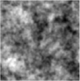
First, the Gaussian background is generated with the power spectrum computed by CMBFAST [27] with sample parameters $\Omega_{b}=0.05$, $\Omega_{\textrm{CDM}}=0.95$, $h=0.5$. We show one such map in Fig. 2. The instrumental noise is simulated as a Gaussian field with a white-noise power spectrum. These two maps are mixed, with the noise being a fraction

$$f_{\textrm{noi}}=\frac{\sigma^{2}_{\textrm{noi}}}{\sigma^{2}_{\textrm{G}}+\sigma^{2}_{\textrm{noi}}},$$ (29)

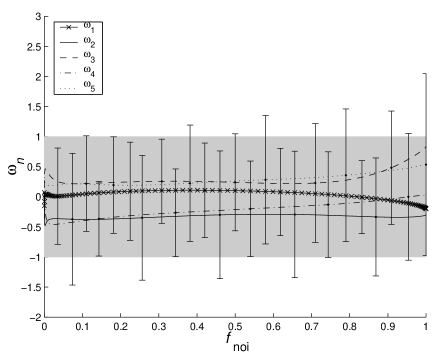
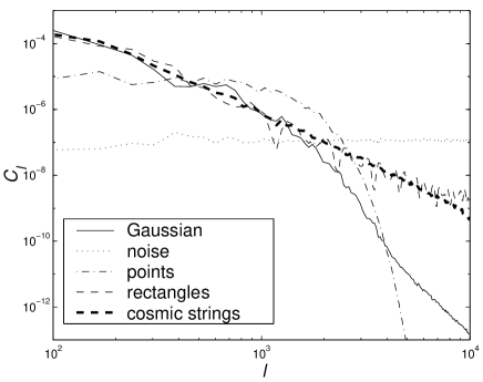
where $\sigma_{\textrm{G}}$ and $\sigma_{\textrm{noi}}$ denote the RMS amplitudes of the Gaussian background and the white noise respectively. We then compute the estimators $\hat{\omega}_{n}$ as defined in Eq. (28), for the value of $f_{\textrm{noi}}$ going from zero to unity. The results are plotted in Fig. 3. Each curve for an estimator $\hat{\omega}_{n}$ is a mean of ten independent realizations with error bars corresponding to the numerically obtained standard deviation of that estimator. The same applies to later figures of this type. For the range $0<f_{\textrm{noi}}<1$, we see that all $\hat{\omega}_{n}$ lie within the one-sigma region $(-1,1)$ and the error bars are well confined within the two-sigma region. This verifies the reliability of our numerical procedure, as well as the theory about the use of $\hat{\omega}_{n}$. For reference, we plot the power spectra of the Gaussian background and the instrumental noise in Fig. 4, as the solid and dotted lines respectively.

FIG. 4.: Power spectra of various components presented in Figs. 2, 5, 7, and 10. Their pixel standard deviations are all made equal to $1$ for comparison purposes.

We generated 10,000 realizations of Gaussian background and computed $\hat{\omega}_{n}$ for each realization. This allowed us to check the probability distributions of $\hat{\omega}_{n}$ numerically, and we find that they are indeed Gaussian distributed with variances all equal to unity for $n=1,...,5$. We have also numerically verified that this result is independent of the underlying power spectrum of the Gaussian background, as it should be on theoretical grounds. One of the advantages of employing $\hat{\omega}_{n}$ for testing Gaussianity is that their theoretical distributions are known, so that one does not need to implement Monte Carlo simulations for the likelihood analysis, i.e. to compute the “equivalent Gaussian realizations” from the map being tested. In the likelihood analyses below we shall simply shade the one-sigma area $-1<\hat{\omega}_{n}<1$ in all relevant plots.

C Point sources

One important challenge for all CMB data analysis is to deal with the presence of point sources. This usually unwanted component obscures the cosmological non-Gaussian signal in most CMB non-Gaussian tests. For this reason it is important to see how this component contributes to our estimators $\hat{\omega}_{n}$.

We first generate five point sources, each having the power spectrum

$$C_{l}\propto\exp\left[-\left(rRk\right)^{2}\right],$$ (30)

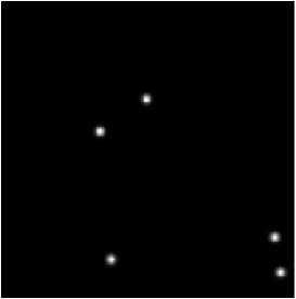
where $R$ is the angular size of the field. Thus $r$ indicates the size of a point as a fraction of the size of the field, and here we use $r=0.01$. A sample map is shown in Fig. 5. The map of point sources is superimposed onto the same Gaussian background as in the previous subsection, with a fraction of the point sources

$$f_{\textrm{pnt}}=\frac{\sigma^{2}_{\textrm{pnt}}}{\sigma^{2}_{\textrm{G}}+\sigma^{2}_{\textrm{pnt}}},$$ (31)

where $\sigma_{\textrm{pnt}}$ is the RMS amplitude of the point signal. We then compute the estimators $\hat{\omega}_{n}(f_{\textrm{pnt}})$ as in the previous case. The results are plotted in Fig. 6.

FIG. 5.: A sample map of random point sources.

FIG. 6.: Estimators $\hat{\omega}_{n}$ of the map of random point sources mixed with the Gaussian background, as functions of the fraction of power in the point sources $f_{\textrm{pnt}}$. The shaded area is $-1<\hat{\omega}_{n}<1$.

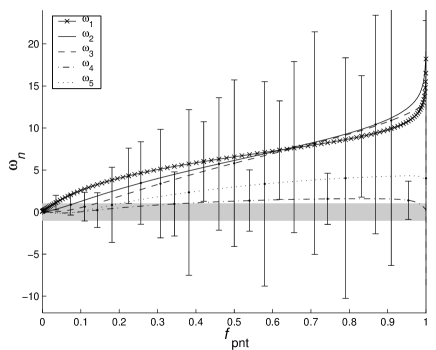
As one can see, when the fraction of the point signal is weak enough ($f_{\textrm{pnt}}\lesssim 0.02$), its non-Gaussianity does not show up. Once this signal becomes stronger ($f_{\textrm{pnt}}\gtrsim 0.02$), $\hat{\omega}_{1}$ starts departing from the one-sigma region while the other $\hat{\omega}_{n}$ follow at larger $f_{\textrm{pnt}}$. With $f_{\textrm{pnt}}\gtrsim 0.1$, one can use $\hat{\omega}_{1}$ to reject the hypothesis of Gaussianity at a confidence level of more than $99\%$, since the solid line with crosses goes outside the three-sigma range $(-3,3)$.

We plotted the power spectrum of the point sources as the dot-dashed line in Fig. 4. By comparing this line to the solid line (the power spectrum of the Gaussian background), we find that for $f_{\textrm{pnt}}\lesssim 0.02$, the point signal never comes to dominate on any scale and so unsurprisingly passes the Gaussianity test using $\hat{\omega}_{n}$. Once $f_{\textrm{pnt}}\gtrsim 0.02$, the power spectrum of the point signal starts to dominate at $l\approx 2000$, at which stage it fails the test. Thus, we conclude that our estimators $\hat{\omega}_{n}$ are sensitive to point sources. For this method to succeed in real CMB data, therefore, it will be necessary to first remove the point sources using any of the available methods (see e.g. [28]), and then compute the estimators $\hat{\omega}_{n}$. In the following analyses, we shall ignore the point sources by assuming that they have been removed beforehand.

D Test on filled rectangles

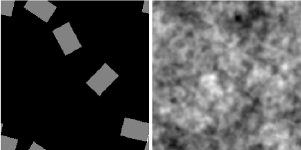
To test the sensitivity of our method to certain types of non-Gaussianity, we first try a simple model using filled rectangles. In a $(5^{\circ})^{2}$ field with a resolution of $256^{2}$ pixels, we generate five filled rectangles, each having a size of $32\times 48$ grid spacings. These rectangles are shown in Fig. 7. This map is then mixed with the Gaussian background used in Fig. 3, with the fraction of rectangles $f_{\textrm{rect}}$ defined similarly to the fraction of point sources $f_{\textrm{pnt}}$. We then computed the estimators $\hat{\omega}_{n}(f_{\textrm{rect}})$ as before, and the results are plotted in Fig. 8.

FIG. 7.: A sample map of filled rectangles (left) and the same map mixed with a Gaussian background with a fraction of power in the rectangles $f_{\textrm{rect}}=0.0005$ (right).

FIG. 8.: Plot of the estimators $\hat{\omega}_{n}$ of the mixed map of rectangles with Gaussian background as a function of $f_{\textrm{rect}}$. The shaded area is $-1<\hat{\omega}_{n}<1$.

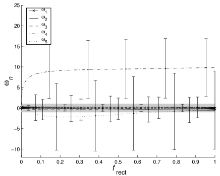
We find that one can use $\hat{\omega}_{4}$ to reject the hypothesis of Gaussianity at more than a 95% confidence level when $f_{\textrm{rect}}\gtrsim 0.001$. This means that non-Gaussian features of the rectangles show up once their RMS amplitude is larger than a few percent of the total amplitude. Referring to the power spectrum of the rectangles in Fig. 4 (the dashed line), we see that once $f_{\textrm{rect}}\lesssim 0.001$, the power of the rectangles never comes to dominate when compared with the power of the Gaussian background (the solid line). This explains why non-Gaussian features of the rectangles are not visible in $\hat{\omega}_{n}$ when $f_{\textrm{rect}}\lesssim 0.001$.

We also test the sensitivity of our method to the rectangles in the presence of noise. In this case we mix three components: the rectangles, the Gaussian background, and the white noise. The last two components are exactly the same as the two we used in Section IV B. The noise fraction is fixed as $f_{\textrm{noi}}=0.05^{2}$, so the rectangles have a fraction

$$f_{\textrm{rect}}=\frac{\sigma^{2}_{\textrm{rect}}}{\sigma^{2}_{\textrm{rect}}+\sigma^{2}_{\textrm{G}}+\sigma^{2}_{\textrm{noi}}}=1-0.05^{2}-f_{\textrm{G}}\,.$$ (32)

The $\hat{\omega}_{n}$ are computed as a function of $f_{\textrm{rect}}$, and the results are presented in Fig. 9.

FIG. 9.: Same as Fig. 8 but mixed with noise with the fraction of power $f_{\textrm{noi}}=0.05^{2}$.

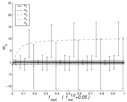
This time we see that the non-Gaussian feature of the rectangles does not show up until a higher $f_{\textrm{rect}}$. For example, one can use $\hat{\omega}_{4}$ to reject the hypothesis of Gaussianity at more then 95% confidence level only when $f_{\textrm{rect}}\gtrsim 0.02$. Referring to the power spectra of the rectangles, the Gaussian background, and the noise in Fig. 4, one finds that when $f_{\textrm{rect}}\lesssim 0.02$ with $f_{\textrm{noi}}=0.05^{2}$, the power of the rectangles is dominated by the power of the Gaussian components (the Gaussian background and the noise); but when $f_{\textrm{rect}}\gtrsim 0.02$, the power in rectangles starts to dominate at $l\approx 4000$. This verifies again that for $\hat{\omega}_{n}$ to succeed in detecting a non-Gaussian signal, the power of the the non-Gaussian component needs to dominate within at least a certain range of the accessible $l$. Thus we see that noise may reduce the sensitivity of our method for detecting non-Gaussian signals, depending on whether the noise dominates the non-Gaussian signal on scales where it originally dominated.

E Detecting cosmic strings

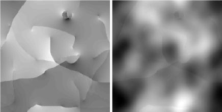
Finally, we test our method against the string-induced CMB map. We use a toy model of Ref. [25] to simulate the string-induced integrated Sachs-Wolfe (ISW) effect. This model incorporates most main features of cosmic strings, such as the scaling and self-avoiding properties, as well as their wiggliness. One realization of the resulting CMB is shown in Fig. 10. The dynamic range is $40$ in conformal time starting from last scattering, and the angular size is $(1^{\circ})^{2}$ with a resolution of $256^{2}$. A Gaussian background is simulated as before. These two maps are then linearly summed, with a string fraction $f_{\textrm{str}}$ defined as above. The estimators $\hat{\omega}_{n}$ are calculated as functions of $f_{\textrm{str}}$, and the results are shown in Fig. 11.

FIG. 10.: Sample $(1^{\circ})^{2}$ maps of the string-induced ISW effect (left) and the same with added Gaussian background (right) where the fraction of power in the string component is $f_{\textrm{str}}=0.0001$.

FIG. 11.: Estimators $\hat{\omega}_{n}$ of the map of strings mixed with a Gaussian background as functions of $f_{\textrm{str}}$. The shaded area is $-1<\hat{\omega}_{n}<1$.

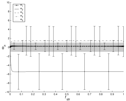
From the solid line in the figure ($\hat{\omega}_{2}$), one can reject the hypothesis of Gaussianity at more than a 95% confidence level when $f_{\textrm{str}}\gtrsim 0.001$. The power spectrum of the Gaussian background is shown as the solid line in Fig. 4, while that of the string-induced ISW effect is shown with the thick dashed line in the same plot. Again, if we compare these two lines, we find that when $f_{\textrm{str}}\lesssim 0.001$, the string-induced perturbations are dominated by the Gaussian background on all scales; when $f_{\textrm{str}}\gtrsim 0.001$, the string-induced perturbations start to dominate at $l\sim 10^{4}$. This result is consistent with our previous argument about the sensitivity of the estimators $\hat{\omega}_{n}$.

In the presence of instrumental noise, this sensitivity will be reduced if the noise dominates the string-induced perturbations on scales where they originally dominated. In other words, the presence of the noise will contribute extra power to the Gaussian component of the underlying map, so as to raise the threshold in power beyond which the non-Gaussian signal may dominate. This argument is again verified in Fig. 12, where we mix three components: the string-induced ISW effect, the Gaussian background, and the white noise whose strength is $5\%$ of the total RMS amplitude. This gives

$$f_{\textrm{str}}=\frac{\sigma^{2}_{\textrm{str}}}{\sigma^{2}_{\textrm{str}}+\sigma^{2}_{\textrm{G}}+\sigma^{2}_{\textrm{noi}}}=1-0.05^{2}-f_{\textrm{G}}\,.$$ (33)

As one can see, the hypothesis of Gaussianity is rejected at more than a 95% confidence level when $f_{\textrm{str}}\gtrsim 0.05$, using $\hat{\omega}_{2}$. This threshold $f_{\textrm{str}}\approx 0.05$ can be again verified by comparing the thick dashed, solid, and dotted lines in Fig. 4.

FIG. 12.: Same as Fig. 11 but for maps mixed with noise, with a noise fraction $f_{\textrm{noi}}=0.05^{2}$.

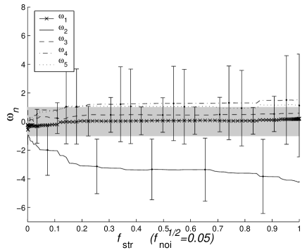
By comparing results for strings and rectangles (see section IV D), we find that they have similar thresholds for rejecting the hypothesis of Gaussianity. This is because strings and rectangles have almost identical power spectra and they dominate the Gaussian component above similar thresholds and at similar scales.

By comparing Figs. 11 and 12, with Figs. 6, 8 and 9, we find that only string-induced perturbations result in a significantly negative value of the estimator $\hat{\omega}_{2}$, while all other non-Gaussian components we tried produce only positive $\hat{\omega}_{n}$ outside the 95% confidence region (the two-sigma region). This provides a potential discriminator in distinguishing string-induced features from other non-Gaussian signals.

V Conclusion

In this paper, we studied the properties of normalized inter-scale cumulants of Fourier modes for homogeneous random fields and proposed a new set of statistics to test a small-scale CMB map for Gaussianity. We showed that higher-order cumulant estimators of Fourier components of Gaussian fields are themselves nearly Gaussian distributed variables with zero expectation value and known variances. Therefore, a test of Gaussianity of these cumulant estimators computed from a given map constitutes a test of Gaussianity of the map. This method is quite general and can be employed on cumulants of any order. However, since the usefulness of higher-order cumulants quickly drops with the order, the bispectrum components and the 4-th order correlators are the most promising candidates.

As an application, the statistical estimators that we denoted by $\hat{\omega}_{n}$ were constructed from all available bispectrum components. We prepared simulated maps made up of random point sources, random rectangles, and simulated cosmic string networks, superimposed on Gaussian background and pixel noise. By developing an analytic model of fields containing random superimposed shapes, we showed that inter-scale cumulants of all orders are generically present in such fields, and that noise and Gaussian background limits the sensitivity of the cumulant estimators on scales where its power spectrum is significant compared to the power spectrum of the non-Gaussian component.

We numerically verified that the discriminators $\hat{\omega}_{n}$ are sensitive to non-Gaussian signal of simulated maps, as well as to point sources. To apply these statistics to detect certain types of non-Gaussian signals such as those resulting from defects, one needs therefore to remove point sources on scales where they dominate the non-Gaussian components one would like to detect. The instrumental noise was also shown to be capable of reducing the sensitivity of our new method, due to its extra contribution to the Gaussian component on small scales. Nevertheless, as we theoretically showed and numerically verified, our new statistics are capable of detecting non-Gaussian component as long as its power spectrum dominates within some range of accessible scales. We also found that the string-induced ISW effect, unlike other non-Gaussian models we tested, such as point sources, induces a significantly negative value of $\hat{\omega}_{2}$. This is a potential discriminator of string-induced perturbations. We intend to apply this method to characterize the non-Gaussian features resulting from more realistic defect models. Even if defects are unimportant as the underlying mechanism for structure formation, we could still apply these methods to detect their existence, especially when high-accuracy and high-resolution observations become available in the near future.

VI Acknowledgments

The authors are grateful to Andrew Liddle, Paul Shellard, and Neil Turok for useful comments and to Alan Heavens, João Magueijo, and Dmitry Pogosian for helpful discussions. A considerable part of this work was completed at DAMTP, University of Cambridge, Cambridge CB3 9EW, U.K. S. W. is supported by DOE and J.-H. P. W. is funded by NSF KDI Grant (9872979) and NASA LTSA Grant (NAG5-6552).C.

A Distribution of cumulant estimators for independent Gaussian samples

To test whether a random variable $x$ is Gaussian distributed, one can estimate higher-order cumulants $\chi_{n}$, $n>2$ of that variable and check that they vanish within their statistical variance. Given a number of realizations of $x$, one can compute moment estimators $\hat{\mu}_{n}$ and cumulant estimators $\hat{\chi}_{n}$ for that purpose. However, obtaining the likelihood that the data $x_{i}$ satisfies the hypothesis requires knowledge of the distribution of the cumulant estimators $\hat{\chi}_{n}$ for an underlying hypothetical Gaussian ensemble of realizations of $x$. If the cumulant estimators $\hat{\chi}_{n}$ were themselves Gaussian distributed, one would only need to know their ensemble mean values $\left\langle\hat{\chi}_{n}\right\rangle$ and covariances $\left\langle\hat{\chi}_{m}\hat{\chi}_{n}\right\rangle$.

In this Appendix we give a self-contained derivation for the covariances of the cumulant estimators $\hat{\chi}_{m}$ computed for a set of $N$ independent samples of one (Gaussian) random variable $x$ with mean $\mu$ and standard deviation $\sigma$. We show below that to leading order in $N^{-1}$, the cumulant estimators are biased by

$$\left\langle\hat{\chi}_{2n}\right\rangle = \chi_{2n}-N^{-1}\frac{\left(2n\right)!}{2n!}\sigma^{2n}+O\left(N^{-2}\right),$$ (A1)

$$\left\langle\hat{\chi}_{2n+1}\right\rangle = \chi_{2n+1}+O\left(N^{-2}\right),$$ (A2)

and are statistically independent,

$$\left\langle\hat{\chi}_{m}\hat{\chi}_{n}\right\rangle-\left\langle\hat{\chi}_{m}\right\rangle\left\langle\hat{\chi}_{n}\right\rangle=N^{-1}\sigma^{2n}n!\delta_{mn}+O\left(N^{-2}\right).$$ (A3)

Here $\chi_{1}=\mu$, $\chi_{2}=\sigma^{2}$ and $\chi_{n}=0$ for $n\geq 3$. We shall also show that the higher-order correlations between $\chi_{n}$ such as $\left\langle\hat{\chi}_{l}\hat{\chi}_{m}\hat{\chi}_{n}\right\rangle$ are absent up to terms of order $O\left(N^{-2}\right)$ and therefore for large $N$ these estimators can be treated as approximately Gaussian distributed, independent random variables with known means and variances. This is immediately relevant to inter-scale cumulants of Fourier space amplitudes, and by using our formalism we show that these are also independent.

Consider a set of $N$ independent realizations $x_{i}$, $i=1,...,N$ of the Gaussian random variable $x$. This set satisfies

$$\left\langle x_{i}\right\rangle=\mu,\quad\left\langle x_{i}x_{j}\right\rangle=\mu^{2}+\sigma^{2}\delta_{ij}.$$ (A4)

The problem at hand is to characterize the estimators for the cumulants $\chi_{n}$ of the distribution of $x$. First we take the unbiased estimators $\hat{\mu}_{n}$ of the moments of $x$, which are

$$\hat{\mu}_{n}\equiv N^{-1}\sum_{i}x_{i}^{n}.$$ (A5)

The cumulant estimators $\hat{\chi}_{n}$ may be defined through these moment estimators by the usual formulae relating cumulants and moments, e.g. for the second and third cumulants

$$\hat{\chi}_{2}=\hat{\mu}_{2}-\hat{\mu}_{1}^{2},$$ (A6)

$$\hat{\chi}_{3}=\hat{\mu}_{3}-3\hat{\mu}_{2}\hat{\mu}_{1}+2\hat{\mu}_{1}^{3},$$ (A7)

and so on (these standard relations follow from Eqs. (A12)-(A14) below). Defined in this manner, the cumulant estimators $\hat{\chi}_{n}$ are however not unbiased, because for instance $\hat{\mu}_{1}^{2}$ in Eq. (A6) is a biased estimator for the square of the first moment $\mu_{1}^{2}$:

$$\left\langle\hat{\mu}_{1}^{2}\right\rangle=\left\langle N^{-2}\sum_{ij}x_{i}x_{j}\right\rangle=\mu_{1}^{2}+N^{-1}\sigma^{2}.$$ (A8)

We shall show now that the resulting bias in $\hat{\chi}_{n}$ is always of order $N^{-1}$ or smaller.

We need to consider this bias in more detail since the expectation values of $\chi_{n}$ are zero for $n>2$ and also because terms of order $O\left(N^{-1}\right)$ dominate the variance of the estimators $\hat{\chi}_{n}$. Terms of order $O\left(N^{-1}\right)$ arise in expressions such as Eq. (A6) from products of moment estimators. By analogy with Eq. (A8) one obtains

$$\left\langle\hat{\mu}_{a}\hat{\mu}_{b}\right\rangle=\mu_{a}\mu_{b}+N^{-1}\left(\mu_{a+b}-\mu_{a}\mu_{b}\right).$$ (A9)

Products of more than two moment estimators will also contain terms of higher order than $N^{-1}$ but here we are only interested in the leading terms. For products of three moments, we obtain

$$\left\langle\hat{\mu}_{a}\hat{\mu}_{b}\hat{\mu}_{c}\right\rangle=\mu_{a}\mu_{b}\mu_{c}+N^{-1}\left(\mu_{a+b}\mu_{c}+\mu_{b+c}\mu_{a}+\mu_{c+a}\mu_{b}-3\mu_{a}\mu_{b}\mu_{c}\right)+O\left(N^{-2}\right),$$ (A10)

and it is straightforward to generalize to products of $k$ estimators,

$$\left\langle\hat{\mu}_{a_{1}}...\hat{\mu}_{a_{k}}\right\rangle=\mu_{a_{1}}...\mu_{a_{k}}+N^{-1}\sum_{1\leq i<j\leq k}\left[\mu_{a_{1}}...\mu_{a_{i}+a_{j}}...\mu_{a_{k}}-\mu_{a_{1}}...\mu_{a_{k}}\right]+O\left(N^{-2}\right).$$ (A11)

The sum above is performed over all pairs of moments entering the original expression.

Now we need to find out where and how such terms appear in expressions for cumulant estimators. The relation of cumulants $\chi_{n}$ to moments $\mu_{n}$ is most easily understood by means of the generating function of moments (also called the characteristic function) $Z\left[p\right]$ which satisfies

$$\mu_{n}=\frac{1}{Z\left[0\right]}\left(i\frac{\partial}{\partial p}\right)^{n}Z\left[p\right]_{p=0}.$$ (A12)

Because of the normalization $Z\left[0\right]^{-1}$ the generating function $Z\left[p\right]$ is defined up to an irrelevant constant factor. For instance, the Gaussian distribution from Eq. (A4) has the generating function

$$Z\left[p\right]=\exp\left[-\frac{p^{2}}{2}\sigma^{2}-i\mu p\right].$$ (A13)

The cumulants can be expressed (or, equivalently, defined) as

$$\chi_{n}=\left(i\frac{\partial}{\partial p}\right)^{n}\ln Z\left[p\right]_{p=0}$$ (A14)

(note that the constant factor in the definition of $Z\left[p\right]$ drops out). The $n$-th derivative of $\ln Z\left[p\right]$ in Eq. (A14) will contain terms such as

$$\frac{1}{Z\left[p\right]}\frac{\partial^{l}Z\left[p\right]}{\partial p^{l}}...\frac{1}{Z\left[p\right]}\frac{\partial^{m}Z\left[p\right]}{\partial p^{m}}$$ (A15)

which give rise to products of moments $\mu_{l}...\mu_{m}$. We would like to replace the moments $\mu_{n}$ by their estimators $\hat{\mu}_{n}$ and then to combine them pairwise to obtain the $O\left(N^{-1}\right)$ terms as shown in Eq. (A11).

We notice that if we take an expression such as $\left(1+N^{-1/2}\mu_{1}\right)...\left(1+N^{-1/2}\mu_{k}\right)$ and expand it in $N^{-1/2}$, then the term of order $O\left(N^{-1}\right)$ will be equal to the sum over all pairs of the product $\mu_{i}\mu_{j}$. This is almost what is required by Eq. (A11), except that we also need to somehow convert $\mu_{i}\mu_{j}$ into $\mu_{i+j}$. This would happen if $\mu_{n}$ behaved like a differential operator $\left(\partial/\partial t\right)^{n}$ acting on functions of a dummy variable $t$. The required technical trick is implemented as follows. We first replace the moments $\mu_{n}$ in Eq. (A14) by the differential operator $\left(\mu_{n}+N^{-1/2}\left[i\partial/\partial t\right]^{n}\right)$. This is done by changing the generating function of moments $Z\left[p\right]$ to

$$\tilde{Z}\left[p;t\right]\equiv\sum_{n=0}^{\infty}\frac{\left(-ip\right)^{n}}{n!}\left(\mu_{n}+N^{-1/2}i^{n}\frac{\partial^{n}}{\partial t^{n}}\right)=Z\left[p\right]+N^{-1/2}\exp\left[p\partial_{t}\right].$$ (A16)

Then we introduce another copy of the old generating function of moments, $Z\left[t\right]$, on which this new generating function $\tilde{Z}\left[p;t\right]$ will act with $\partial_{t}$ at the end of the calculation, so that the derivatives $\left[i\partial_{t}\right]^{n}$ will at the end be replaced again by the moments $\mu_{n}$. We now claim that the expectation value of cumulant estimators $\hat{\chi}_{n}$ and of their products can be obtained up to and including terms of order $O\left(N^{-1}\right)$ from the modified generating function $\tilde{Z}\left[p;t\right]$ as

$$\left\langle\hat{\chi}_{n}\right\rangle=\left[i\partial_{p}\right]^{n}\ln\tilde{Z}\left[p;t\right]Z\left[t\right]_{p=t=0}+O\left(N^{-3/2}\right)$$ (A17)

and

$$\left\langle\hat{\chi}_{m}\hat{\chi}_{n}\right\rangle=\left(\left[i\partial_{p^{\prime}}\right]^{m}\ln\tilde{Z}\left[p^{\prime};t\right]\right)\left(\left[i\partial_{p}\right]^{n}\ln\tilde{Z}\left[p;t\right]\right)Z\left[t\right]_{p=p^{\prime}=t=0}+O\left(N^{-3/2}\right).$$ (A18)

Here the parameters $p$, $p^{\prime}$ and $t$ are set to $0$ only after all derivatives have been computed. Expectation values of products of three or more cumulant estimators $\hat{\chi}_{n}$ are be obtained in the same manner,

$$\left\langle\hat{\chi}_{n_{1}}...\hat{\chi}_{n_{k}}\right\rangle=\left(\left[i\partial_{p_{1}}\right]^{n_{1}}\ln\tilde{Z}\left[p_{1};t\right]\right)...\left(\left[i\partial_{p_{k}}\right]^{n_{k}}\ln\tilde{Z}\left[p_{k};t\right]\right)Z\left[t\right]_{p_{j}=t=0}+O\left(N^{-3/2}\right).$$ (A19)

We shall first show that Eqs. (A17)-(A18) actually give the desired $O\left(N^{-1}\right)$ terms and then proceed to compute these terms.

Consider Eq. (A17): after evaluating all derivatives in $p$ we would obtain many terms of the form of Eq. (A15) but with the modified generating function $\tilde{Z}\left[p;t\right]$ acting (with the derivatives in $t$) on $Z\left[t\right]$,

$$\left(\frac{1}{\tilde{Z}\left[p;t\right]}\frac{\partial^{l_{1}}\tilde{Z}\left[p;t\right]}{\partial p^{l_{1}}}...\frac{1}{\tilde{Z}\left[p;t\right]}\frac{\partial^{l_{n}}\tilde{Z}\left[p;t\right]}{\partial p^{l_{n}}}\right)_{p=0}Z\left[t\right]_{t=0}.$$ (A20)

Take one such term, substitute $p=0$ and expand in $N^{-1/2}$:

$\displaystyle\left(\frac{1}{\tilde{Z}\left[p;t\right]}\frac{\partial^{l_{1}}\tilde{Z}\left[p;t\right]}{\partial p^{l_{1}}}...\frac{1}{\tilde{Z}\left[p;t\right]}\frac{\partial^{l_{n}}\tilde{Z}\left[p;t\right]}{\partial p^{l_{n}}}\right)_{p=0}Z\left[t\right]_{t=0}$

$\displaystyle=\frac{\mu_{l_{1}}+N^{-1/2}\left(i\partial_{t}\right)^{l_{1}}}{1+N^{-1/2}}...\frac{\mu_{l_{n}}+N^{-1/2}\left(i\partial_{t}\right)^{l_{n}}}{1+N^{-1/2}}Z\left[t\right]_{t=0}$

$\displaystyle=\mu_{l_{1}}...\mu_{l_{n}}+N^{-1/2}\left(-n\mu_{l_{1}}...\mu_{l_{n}}+\sum_{k=1}^{n}\mu_{l_{1}}...\left(i\partial_{t}\right)^{l_{k}}...\mu_{l_{n}}\right)Z\left[t\right]_{t=0}$

$$+N^{-1}\left(-\frac{n\left(n-1\right)}{2}\mu_{l_{1}}...\mu_{l_{n}}+\sum_{1\leq i<j\leq n}\mu_{l_{1}}...\left(i\partial_{t}\right)^{l_{i+j}}...\mu_{l_{n}}\right)Z\left[t\right]_{t=0}+O\left(N^{-3/2}\right).$$ (A21)

Note that after taking the derivatives in $t$ the $O\left(1\right)$ and $O\left(N^{-1}\right)$ terms in Eq. (A21) are exactly the ones in Eq. (A11), while the $O\left(N^{-1/2}\right)$ terms cancel. Therefore each term of the form of Eq. (A20) yields the desired combination of moments for Eq. (A17). Note that although the modified generating function $\tilde{Z}\left[p;t\right]$ gives the correct result in the $O\left(N^{-1}\right)$ terms, its higher-order expansion terms are not useful.

The same argument can be shown to hold for Eq. (A18) and generally for analogous expressions for averages of products of several $\hat{\chi}_{n}$. We only need to take all derivatives in the parameters $p$, $p^{\prime}$, … prior to taking the derivative in $t$ in those expansions.

Our strategy to obtain the expectation values from Eqs. (A17)-(A18) will be to first expand in $N^{-1/2}$ up to $O\left(N^{-1}\right)$, then substitute $p=0$ in the correct order, and then evaluate the derivatives in $t$. Since we know that the $O\left(1\right)$ terms give the unbiased result and that terms of order $O\left(N^{-1/2}\right)$ vanish (both of these statements are straightforwardly checked by a similar calculation), while the $O\left(N^{-3/2}\right)$ and higher-order terms are not useful for us, we only concentrate on the $O\left(N^{-1}\right)$ terms. Expanding the logarithm in Eq. (A16),

$$\ln\tilde{Z}\left[p;t\right]=\ln Z\left[p\right]+N^{-1/2}\frac{\exp\left[p\partial_{t}\right]}{Z\left[p\right]}-\frac{N^{-1}}{2}\frac{\exp\left[2p\partial_{t}\right]}{Z\left[p\right]^{2}}+O\left(N^{-3/2}\right),$$ (A22)

we obtain the expression

$$\ln\tilde{Z}\left[p;t\right]Z\left[t\right]=\chi_{n}Z\left[t\right]+N^{-1/2}\frac{Z\left[p+t\right]}{Z\left[p\right]}-\frac{N^{-1}}{2}\frac{Z\left[2p+t\right]}{Z\left[p\right]^{2}}+O\left(N^{-3/2}\right),$$ (A23)

which will give the answer to Eq. (A17) if we take the derivative in $p$ and substitute $p=t=0$. The result is

$$\left\langle\hat{\chi}_{n}\right\rangle=\chi_{n}-\frac{N^{-1}}{2}\left[i\partial_{p}\right]_{p=0}^{n}\frac{Z\left[2p\right]}{Z\left[p\right]^{2}}+O\left(N^{-2}\right).$$ (A24)

At this point we need to use a particular generating function $Z\left[p\right]$. For a Gaussian variable with the generating function given by Eq. (A13) the expectation value becomes

$$\left\langle\hat{\chi}_{n}\right\rangle=\chi_{n}-\frac{N^{-1}}{2}\left[i\partial_{p}\right]_{p=0}^{n}e^{-\sigma^{2}p^{2}}+O\left(N^{-2}\right).$$ (A25)

This is the same as Eqs. (A1)-(A2).

Eq. (A24) expresses the cumulant estimator bias for an arbitrary distribution through its generating function $Z\left[p\right]$. Although it can be seen that the bias for a non-Gaussian distribution will be different from that of Eq. (A25), we do not need its general expression since we are only interested in testing the hypothesis of an underlying Gaussian distribution.

The calculation of the covariances of cumulants (Eq. (A18)) is a little more involved since we need to expand both logarithmic terms prior to taking the derivatives in $t$. We begin with one logarithmic term [cf. Eq. (A23)], use the Gaussian generating function $Z\left[t\right]$ and evaluate the $n$-th derivative in $p$ while keeping the $t$ variable intact,

$$\left[i\partial_{p}\right]^{n}\left(Z\left[t\right]\ln Z\left[p\right]+N^{-1/2}Z\left[t\right]\exp\left(-\sigma^{2}pt\right)-\frac{N^{-1}}{2}Z\left[t\right]\exp\left(-\sigma^{2}p^{2}-2\sigma^{2}pt\right)\right)$$ (A26)

$$= Z\left[t\right]\chi_{n}+N^{-1/2}Z\left[t\right]\left(-i\right)^{n}\sigma^{2n}t^{n}-\frac{N^{-1}}{2}Z\left[t\right]\left[i\partial_{p}\right]_{p=0}^{n}\exp\left(-\sigma^{2}p^{2}-2\sigma^{2}pt\right).$$ (A27)

(We shall not need the full expansion of the last cumbersome derivative.) Then we act on this expression with another logarithmic term (from Eq. (A22)), set $t=0$ and take the $m$-th derivative in $p$. After some straightforward algebra we obtain Eq. (A3):

$$\left\langle\hat{\chi}_{m}\hat{\chi}_{n}\right\rangle-\left\langle\hat{\chi}_{m}\right\rangle\left\langle\hat{\chi}_{n}\right\rangle=N^{-1}\left[i\partial_{p}\right]_{p=0}^{m}\left(-i\right)^{n}\sigma^{2n}p^{n}=N^{-1}n!\sigma^{2n}\delta_{mn}+O\left(N^{-2}\right).$$ (A28)

The same method and Eq. (A24) can be used to compute the expectation values and covariances of cumulant estimators also for non-Gaussian distributions as long as the generating function $Z\left[p\right]$ is given. Expectation values of products of two or more cumulants (e.g. $\left\langle\hat{\chi}_{l}\hat{\chi}_{m}\hat{\chi}_{n}\right\rangle$) can be found as well, although the calculations are cumbersome. However, in the case of the underlying Gaussian distribution a simple algebraic consideration shows that higher-order correlations between the cumulant estimators $\hat{\chi}_{n}$ are of order $O\left(N^{-2}\right)$ or smaller, and therefore $\hat{\chi}_{n}$ themselves can be approximately treated as independent Gaussian variables. This is found by noticing that the logarithmic derivative operator of Eq. (A22) contains terms of order $O\left(N^{-1/2}\right)$ and $O\left(N^{-1}\right)$ while we are only interested in the $O\left(N^{-1}\right)$ terms in the final result. We could introduce a formal operator $L_{n}$ by

$$L_{n}\equiv\left[i\partial_{p}\right]^{n}\ln\tilde{Z}\left[p,t\right]_{p=0}=\chi_{n}+N^{-1/2}A_{n}+N^{-1}B_{n}+O\left(N^{-3/2}\right).$$ (A29)

The operator coefficients $A_{n}$ and $B_{n}$ will later act on $Z\left[t\right]$ with their derivatives in $t$ evaluated only at the end; note that $A_{n}Z\left[t\right]_{t=0}=0.$ Then Eq. (A18) for the correlation between the cumulant estimators is rewritten as

$$\left\langle\hat{\chi}_{m}\hat{\chi}_{n}\right\rangle=L_{m}L_{n}Z\left[t\right]_{t=0}+O\left(N^{-3/2}\right).$$ (A30)

Selecting the $O\left(N^{-1}\right)$ terms in the product gives

$$L_{m}L_{n}Z\left[t\right]_{t=0}-\left(L_{m}Z\left[t\right]_{t=0}\right)\left(L_{n}Z\left[t\right]_{t=0}\right)=N^{-1}A_{m}A_{n}Z\left[t\right]_{t=0}+...$$ (A31)

where all terms containing $B_{n}$ cancel. The only surviving $O\left(N^{-1}\right)$ term came from the product of two $O\left(N^{-1/2}\right)$ non-commuting operator terms, and all other terms contained a commuting $\chi_{n}$ and canceled after subtracting the product of the expectation values. Now we notice that the $O\left(N^{-1}\right)$ terms in a product of more than two operators $L_{n}$ from Eq. (A29) must contain at least one factor $\chi_{n}$. It follows that all “connected correlators” of more than two cumulant estimators, such as

$$\left\langle\hat{\chi}_{l}\hat{\chi}_{m}\hat{\chi}_{n}\right\rangle-\left\langle\hat{\chi}_{l}\right\rangle\left\langle\hat{\chi}_{m}\hat{\chi}_{n}\right\rangle-\left\langle\hat{\chi}_{m}\right\rangle\left\langle\hat{\chi}_{l}\hat{\chi}_{n}\right\rangle-\left\langle\hat{\chi}_{n}\right\rangle\left\langle\hat{\chi}_{l}\hat{\chi}_{m}\right\rangle+2\left\langle\hat{\chi}_{l}\right\rangle\left\langle\hat{\chi}_{m}\right\rangle\left\langle\hat{\chi}_{n}\right\rangle$$ (A32)

(for any $l$, $m$, $n$) contain no $O\left(N^{-1}\right)$ terms. Therefore the cumulant estimators $\hat{\chi}_{n}$ in the limit of large number of samples $N$ are approximately Gaussian distributed and independent variables (up to terms of order $O\left(N^{-2}\right)$).

B Properties of multivariate cumulants

Here we examine the estimators $\hat{\chi}_{mn}$ of cumulants of a distribution of two Gaussian variables $\left(x,y\right)$ which are independent and have variances $\sigma_{x}^{2}$ and $\sigma_{y}^{2}$. We show that the cumulant estimators are approximately independent in the limit of large sample size $N$, namely that their covariances are

$$\left\langle\hat{\chi}_{kl}\hat{\chi}_{mn}\right\rangle-\left\langle\hat{\chi}_{kl}\right\rangle\left\langle\hat{\chi}_{mn}\right\rangle=N^{-1}m!n!\,\delta_{km}\delta_{ln}\sigma_{x}^{2m}\sigma_{y}^{2n}+O\left(N^{-2}\right),$$ (B1)

while the means are biased by a quantity of order $N^{-1}$,

$$\left\langle\hat{\chi}_{kl}\right\rangle=O\left(N^{-1}\right).$$ (B2)

Then we show how to generalize the results of the previous Appendix to multivariate cumulants.

Cumulants of a distribution of two variables $\left(x,y\right)$ are defined by analogy with Eq. (A14),

$$\chi_{mn}=\left[i\partial_{p}\right]^{m}\left[i\partial_{q}\right]^{n}\ln Z\left[p,q\right]_{p=q=0},$$ (B3)

where $Z\left[p,q\right]$ is the generating function of moments of the distribution,

$$\mu_{mn}\equiv\left\langle x^{m}y^{n}\right\rangle=\left[i\partial_{p}\right]^{m}\left[i\partial_{q}\right]^{n}Z\left[p,q\right]_{p=q=0}.$$ (B4)

A Gaussian distribution is characterized by

$$Z\left[p,q\right]=\exp\left[-\frac{1}{2}\left(p,q\right){\mathbf{C}}\left(p,q\right)^{T}\right]$$ (B5)

where we multiplied the row and column $2$-vectors $\left(p,q\right)$ by the appropriate $2\times 2$ correlation matrix ${\mathbf{C}}$. (This matrix is diagonal if the variables $\left(x,y\right)$ are independent, but we shall not need this for most of the derivation.)

We follow the same method of calculation as in Appendix A and introduce a modified (operator-valued) generating function

$$\tilde{Z}\left[p,q;t,u\right]\equiv Z\left[p,q\right]+N^{-1/2}\exp\left[p\partial_{t}+q\partial_{u}\right]$$ (B6)

to be used instead of $\tilde{Z}\left[p,t\right]$ in Eqs. (A17), (A18). We omit the calculations since they are very similar to those in Appendix A and only cite the results. The bias in the cumulant estimators $\hat{\chi}_{mn}$ is described by a formula analogous to Eq. (A25),

$$\left\langle\hat{\chi}_{mn}\right\rangle=\chi_{mn}-\frac{N^{-1}}{2}\left[i\partial_{p}\right]^{m}\left[i\partial_{q}\right]^{n}\exp\left[-\left(p,q\right){\mathbf{C}}\left(p,q\right)^{T}\right]_{p=q=0}.$$ (B7)

The covariance of two cumulant estimators $\hat{\chi}_{kl}$ and $\hat{\chi}_{mn}$ vanishes unless the cumulants are of the same order, $k+l=m+n$, in which case it is given by

$$\left\langle\hat{\chi}_{kl}\hat{\chi}_{mn}\right\rangle-\left\langle\hat{\chi}_{kl}\right\rangle\left\langle\hat{\chi}_{mn}\right\rangle=N^{-1}\left[i\partial_{t}\right]^{k}\left[i\partial_{u}\right]^{l}\left[i\partial_{p}\right]^{m}\left[i\partial_{q}\right]^{n}\exp\left[-\left(t,u\right){\mathbf{C}}\left(p,q\right)^{T}\right]_{p=q=t=u=0}.$$ (B8)

In our case of interest, the covariance matrix ${\mathbf{C}}$ is diagonal,

$$C=\left(\begin{array}[]{cc}\sigma_{x}^{2}&0\\ 0&\sigma_{y}^{2}\end{array}\right),$$ (B9)

and then Eqs. (B7)-(B8) simplify to

$$\left\langle\hat{\chi}_{mn}\right\rangle=\chi_{mn}-\frac{N^{-1}}{2}\left[i\partial_{p}\right]^{m}\left[i\partial_{q}\right]^{n}\exp\left[-p^{2}\sigma_{x}^{2}-q^{2}\sigma_{y}^{2}\right]_{p=q=0}+O\left(N^{-2}\right),$$ (B10)

$$\left\langle\hat{\chi}_{kl}\hat{\chi}_{mn}\right\rangle-\left\langle\hat{\chi}_{kl}\right\rangle\left\langle\hat{\chi}_{mn}\right\rangle=N^{-1}m!n!\delta_{km}\delta_{ln}\sigma_{x}^{2m}\sigma_{y}^{2n}+O\left(N^{-2}\right).$$ (B11)

The expressions of Eqs. (B10)-(B11) are straightforwardly generalized for distributions of three and more variables, for example

$$\textrm{var}\left[\hat{\chi}_{klm}\right]=N^{-1}k!l!m!\sigma_{x}^{2k}\sigma_{y}^{2l}\sigma_{z}^{2m}+O\left(N^{-2}\right).$$ (B12)

For the case of cumulants of Fourier components of a Gaussian random field, the individual Fourier modes are independently distributed with variances equal to the power spectrum $P\left(k\right)$. Therefore the expressions we derived are applicable directly with the substitution $\sigma_{x}^{2}=P\left(k_{1}\right)$, $\sigma_{y}^{2}=P\left(k_{2}\right)$,… for the appropriate modes. A general Fourier cumulant $\tilde{C}^{\left(n\right)}\left({\mathbf{k}}_{1},...,{\mathbf{k}}_{n}\right)$ of Eq. (9) with all $n$ vectors ${\mathbf{k}}_{i}$ distinct will be estimated from $N$ samples obtained by rotating the set of vectors $\left\{{\mathbf{k}}_{i}\right\}$ and is in our notation a cumulant $\chi_{11...1}$ of the $n$-variable distribution of the $n$ Fourier modes $a_{{\mathbf{k}}_{i}}$; its sample variance is therefore

$$\textrm{var}\left[\tilde{C}^{\left(n\right)}\left({\mathbf{k}}_{1},...,{\mathbf{k}}_{n}\right)\right]=N^{-1}P\left(k_{1}\right)...P\left(k_{n}\right)+O\left(N^{-2}\right).$$ (B13)

C Generating functionals for random superpositions of shapes

Here we derive the generating functional for the random field resulting from a superposition of fixed profiles (shapes), centered at points (“seeds”) drawn from some known distribution and scaled and rotated randomly. In particular, we show how to use the generating functional to obtain the cumulants of Fourier components for such a random field. We first consider the simpler case of the Poisson distribution of seeds and then briefly show how to generalize the same formalism for non-Poisson distributions of seed centers.

We work in flat space for simplicity; although we only need the result in two dimensions, our derivation applies to any $d$-dimensional space. We consider a finite region of space with unit area, so that $\int dx=1$. If we start with a shape of a given profile $s\left(x\right)$ and translate it to a set of locations $x_{1}$, …, $x_{n}$, the result is

$$f\left(x;x_{1},...,x_{n}\right)=\sum_{k}s\left(x-x_{k}\right).$$ (C1)

To compute the generating functional for the distribution $f\left(x;x_{1},...,x_{n}\right)$ we need to average the following over all numbers $n$ of centers and center positions $x_{k}$:

$$Z\left[J\left(x\right)\right]=\left\langle\exp\left(-i\int f\left(x;x_{1},...,x_{n}\right)J\left(x\right)dx\right)\right\rangle.$$ (C2)

The centers $x_{i}$ are Poisson distributed with a fixed mean number of centers $n_{c}$ in the whole region, and the probability of having $n$ centers is $\left(n_{c}\right)^{n}\exp\left(-n_{c}\right)/n!$. The averaging in Eq. (C2) with $f\left(x\right)$ defined by Eq. (C1) then gives

$$Z\left[J\left(x\right)\right] = e^{-n_{c}}\sum^{\infty}_{n=0}\frac{n_{c}^{n}}{n!}\int dx_{1}...dx_{n}\exp\left(-i\int f\left(x;x_{1},...,x_{n}\right)J\left(x\right)dx\right)$$ (C3)

$$= \exp\left(-n_{c}+n_{c}\int dx_{0}\exp\left(-i\int s\left(x-x_{0}\right)J\left(x\right)dx\right)\right)$$ (C4)

As usual, the logarithm $\ln Z\left[J\left(x\right)\right]$ of the generating functional generates the cumulants $C^{\left(n\right)}\left(x_{1},...,x_{n}\right)$ of the distribution,

$$\ln Z\left[J\left(x\right)\right]=\int C^{\left(1\right)}\left(x_{1}\right)\frac{J\left(x_{1}\right)}{i}dx_{1}+\int C^{\left(2\right)}\left(x_{1},x_{2}\right)\frac{J\left(x_{1}\right)J\left(x_{2}\right)}{i^{2}2!}dx_{1}dx_{2}+...$$ (C5)

(this can also be taken as a definition of cumulants) and therefore is of most interest for us.

We now add more variety to the random field $f\left(x;x_{1},...,x_{n}\right)$ by allowing the shapes $s\left(x\right)$ to be rotated, scaled and attenuated. The rotation is effected by introducing an orthogonal matrix $R$ uniformly distributed in the orthogonal group of $d$-dimensional rotations ${\mathbf{O}}\left(d\right)$; the scaling by a factor $\lambda$ distributed according to some probability density $p_{\lambda}\left(\lambda\right)$; and the attenuation by multiplying the profile by an overall factor $\nu$ with probability density $p_{\nu}\left(\nu\right)$. We give each shape an individual randomly selected rotation angle, scale and attenuation. The transformed profile is $\nu s\left(\lambda^{-1}R\left(x-x_{0}\right)\right)$ and the generating functional is similar to the one above:

$$\ln Z\left[J\left(x\right)\right]=-n_{c}+n_{c}\int dx_{0}dR\,p_{\lambda}\left(\lambda\right)d\lambda\,p_{\nu}\left(\nu\right)d\nu$$ (C6)

$$\times\exp\left(-i\nu\int s\left(\lambda^{-1}R\left(x-x_{0}\right)\right)J\left(x\right)dx\right).$$ (C7)

Here the integration measure $dR$ for rotations is assumed to be normalized to unity, as well as with all other integrations. We shall below drop the irrelevant additive constant $n_{c}$ in Eq. (C7).

The non-Gaussian components of the distribution are now read from Eq. (C7). After the exponential is expanded in powers of $J\left(x\right)$ under the integral, the general cumulant of order $n$ is formed from the terms of order $J\left(x\right)^{n}$ and can be readily found for any given profile $s\left(x\right)$ and any assumed distributions of scaling and attenuation. The resulting non-Gaussian distribution is homogeneous and isotropic due to averaging over spatial position $x_{0}$ and the rotations $R$.

To illustrate the method, we extract from Eq. (C7) the characteristic function $\tilde{f}\left(j\right)$ of the one-point distribution of $f\left(x;x_{1},...,x_{n}\right)$ at a fixed reference point $x=x_{*}$. This is done by substituting $J\left(x\right)=j\delta\left(x-x_{*}\right)$ into Eq. (C7); the result is the generating function of cumulants for the one-point distribution,

$$\ln\tilde{f}\left(j\right)\equiv\sum_{n}\frac{j^{n}}{i^{n}n!}\chi_{n}=n_{c}\left\langle\lambda\right\rangle\int dx\,p_{\nu}\left(\nu\right)d\nu\,\exp\left(-i\nu s\left(x\right)j\right)$$ (C8)

and the $n$-th cumulant $\chi_{n}$ of that distribution is

$$\chi_{n}=n_{c}\left\langle\lambda\right\rangle\left\langle\nu^{n}\right\rangle\left\langle s^{n}\left(x\right)\right\rangle_{x}.$$ (C9)

In the same manner, one can obtain the generating functional for the distribution of the Fourier components of $f\left(x\right)$. By Fourier transforming Eq. (C7) we obtain

$$\ln Z\left[j\left(k\right)\right]=n_{c}\int dx\,dR\,p_{\lambda}\left(\lambda\right)d\lambda\,p_{\nu}\left(\nu\right)d\nu\,\exp\left(-i\nu\int\tilde{s}\left(-\lambda Rk\right)j\left(k\right)e^{-ikx}\frac{dk}{\left(2\pi\right)^{d}}\right).$$ (C10)

The $n$-th Fourier space cumulant $\tilde{C}^{\left(n\right)}\left(k_{1},...,k_{n}\right)$ is then given by

$$\tilde{C}^{\left(n\right)}\left(k_{1},...,k_{n}\right)=n_{c}\left\langle\nu^{n}\right\rangle\int dR\,p_{\lambda}\left(\lambda\right)d\lambda\,\delta\left(k_{1}+...+k_{n}\right)\prod^{n}_{i=1}\tilde{s}\left(-\lambda Rk_{i}.\right)$$ (C11)

Note that since $\tilde{s}\left(k\right)$ is a Fourier transform of a real profile function $s\left(x\right)$ and the rotations $R$ include mirror symmetry $k\rightarrow-k$, the cumulant of Eq. (C11) is always real-valued.

Although Eq. (C11) shows that cumulants of all orders are generally expected to be nonzero, we need to estimate the statistical significance of their deviation from zero compared to the sample variance. The variance of a cumulant estimator, as derived above, is proportional to the appropriate powers of the power spectrum. The power spectrum $P\left(k\right)$ of the seed-induced distribution can be found from Eq. (C11) as the second-order cumulant $\tilde{C}^{\left(2\right)}\left(k,-k\right)$,

$$P\left(k\right)=n_{c}\left\langle\nu^{2}\right\rangle\int dR\,p_{\lambda}\left(\lambda\right)d\lambda\,\left|\tilde{s}\left(-\lambda Rk\right)\right|^{2}.$$ (C12)

To understand the qualitative behavior of the cumulant estimators, we shall simplify the case by assuming that the distribution of scales $p_{\lambda}\left(\lambda\right)$ is trivial and that the profile $s\left(x\right)$ is spherically symmetric. In that case, the integrals in Eqs. (C11), (C12) simplify

$$\tilde{C}^{\left(n\right)}\left(k_{1},...,k_{n}\right)=n_{c}\left\langle\nu^{n}\right\rangle\tilde{s}\left(k_{1}\right)...\tilde{s}\left(k_{n}\right),$$ (C13)

$$P\left(k\right)=n_{c}\left\langle\nu^{2}\right\rangle\left|\tilde{s}\left(k\right)\right|^{2}.$$ (C14)

If the cumulant $\tilde{C}^{\left(n\right)}\left(k_{1},...,k_{n}\right)$ is estimated using a sample of $N$ values, the ratio of the expected signal to the standard deviation of the estimator for a Gaussian sample (assuming all $k_{i}$ are different) is

$$\frac{\tilde{C}^{\left(n\right)}\left(k_{1},...,k_{n}\right)}{\sqrt{\textrm{var}\left[\tilde{C}^{\left(n\right)}\left(k_{1},...,k_{n}\right)\right]}}=\frac{\sqrt{N}}{n_{c}^{n/2-1}}\frac{\left\langle\nu^{n}\right\rangle}{\left\langle\nu^{2}\right\rangle^{n/2}}\frac{\tilde{s}\left(k_{1}\right)...\tilde{s}\left(k_{n}\right)}{\left|\tilde{s}\left(k_{1}\right)\right|...\left|\tilde{s}\left(k_{n}\right)\right|}.$$ (C15)

The last ratio of various $\tilde{s}\left(k\right)$ in Eq. (C15) is equal to $1$ if the homogeneity constraint $k_{1}+...+k_{n}=0$ is satisfied; also the ratio containing $\nu$ should be of order $1$ except for specially engineered attenuation distributions. We obtain therefore the general result that the sensitivity of an individual cumulant estimator is decreased with the cumulant order $n$ and with the expected number $n_{c}$ of seeds in the observation region (the latter is a manifestation of the central limit theorem), and grows with the number $N$ of sample points which is determined by the number of modes $a_{{\mathbf{k}}}$ at the chosen scales as $\sqrt{N}$. We stress that Eq. (C15) provides only an estimate of the sensitivity under simplifying assumptions of spherical symmetry and fixed scale of seed profiles.

Finally, we generalize our formalism to include arbitrary (non-Poisson) distributions of seed centers. Similarly to a continuous random field, a distribution of seed centers can be fully specified by a suitable generating functional. Constructing it is equivalent to specifying all the connected correlation functions $\xi\left(x_{1},...,x_{n}\right)$ of seed positions. Assume that we are given all joint probability densities $Prob\left(x_{1},...,x_{n}\right)\prod_{k}dx_{k}$ for having a seed at each of the positions $x_{1}$,…,$x_{n}$. If we denote the one-point seed density $Prob(x_{1})\equiv n_{s}\left(x_{1}\right)$, then the two-point seed correlation function $\xi\left(x_{1},x_{2}\right)$ is usually defined by

$$Prob(x_{1},x_{2})\equiv n_{s}\left(x_{1}\right)n_{s}\left(x_{2}\right)\left[1+\xi\left(x_{1},x_{2}\right)\right].$$ (C16)

The three-point function $\xi\left(x_{1},x_{2},x_{3}\right)$ is then defined from the relation

$$Prob\left(x_{1},x_{2},x_{3}\right)\equiv n_{s}\left(x_{1}\right)n_{s}\left(x_{2}\right)n_{s}\left(x_{3}\right)\left[1+\xi\left(x_{1},x_{2}\right)\right.$$ (C17)

$$\left.+\xi\left(x_{1},x_{3}\right)+\xi\left(x_{2},x_{3}\right)+\xi\left(x_{1},x_{2},x_{3}\right)\right]$$ (C18)

and similarly for the higher-order correlations. The relation between the joint probability densities $Prob\left(x_{1},...,x_{n}\right)$ and the connected correlation functions $\xi\left(x_{1},...,x_{n}\right)$ is similar to that of moments and cumulants of a continuous random field (except that $\xi$’s in our case are multiplied by several factors of $n_{s}$). We can define the generating functional for the seed distribution $Z_{s}\left[J\left(x\right)\right]$ as the functional that generates the joint probabilities,

$$Z_{s}\left[J\left(x\right)\right]\equiv 1+\sum_{n=1}^{\infty}\int dx_{1}...dx_{n}\frac{J\left(x_{1}\right)...J\left(x_{n}\right)}{i^{n}n!}Prob\left(x_{1},...,x_{n}\right).$$ (C19)

One can see from Eqs. (C16), (C18) that the connected correlation functions $\xi\left(x_{1},x_{2},...\right)$ are generated by the logarithm of $Z_{s}$, similarly to the usual cumulants except for the normalization to the one-point density $n_{s}$:

$$\xi\left(x_{1},...,x_{n}\right)=i^{n}\frac{\delta^{n}}{\delta J\left(x_{1}\right)...\delta J\left(x_{n}\right)}\ln Z_{s}\left[\frac{1}{n_{s}\left(x\right)}J\left(x\right)\right]_{J=0}.$$ (C20)

Conversely, if we are given the full set of connected correlators $\xi\left(x_{1},...,x_{n}\right),\,n\geq 2$, we use Eq. (C20) to construct the generating functional for seeds $Z_{s}\left[J\right]$ (we would need to formally introduce the one-point correlators as $\xi\left(x_{1}\right)\equiv 1$ to use Eq. (C20) with $n=1$ and also fix $Z_{s}\left[J=0\right]=1$).

A simple example is a Poisson distribution where the seeds are completely uncorrelated, $\xi\left(x_{1},...,x_{n}\right)=0$ for $n\geq 2$ and the distribution is completely specified by the seed density $n_{s}\left(x\right)$. We obtain a generating functional

$$Z_{s}^{(\textrm{P})}\left[J\left(x\right)\right]=\exp\left[-i\int n_{s}\left(x\right)J\left(x\right)dx\right].$$ (C21)

It turns out that given any generating functional of seeds $Z_{s}\left[J\right]$, one can directly obtain the generating functional $Z\left[J\right]$ for the “seeded” random field of Eq. (C1). To show this, we compare the definitions of both functionals. The definition of $Z\left[J\right]$ in Eq. (C2) is the average of the quantity

$$\exp\left(-i\int f\left(x;x_{1},...,x_{n}\right)J\left(x\right)dx\right)\equiv\prod_{k=1}^{n}E\left(x_{k};J\right),$$ (C22)

$$E\left(x;J\right)\equiv\exp\left[-i\int J\left(x^{\prime}\right)s\left(x^{\prime}-x\right)dx^{\prime}\right],$$ (C23)

over all seed numbers $n$ and seed positions $x_{k}$. The average is weighed by the probabilities $P\left(x_{1},...,x_{n}\right)\prod_{k}dx_{k}$ of having seeds at points $x_{1}$,…,$x_{n}$ and nowhere else. These probabilities are related to the probability densities $Prob\left(x_{1},...,x_{n}\right)$ by

$$P\left(x_{1},...,x_{n}\right)=P\left(\emptyset\right)Prob\left(x_{1},...,x_{n}\right)$$ (C24)

where $P\left(\emptyset\right)=\exp\left[-\int n_{s}\left(x\right)dx\right]$ is the (finite) probability of having no seeds anywhere. Then Eq. (C2) can be rewritten as

$$Z\left[J\left(x\right)\right]=P\left(\emptyset\right)\left[1+\int dx_{1}Prob\left(x_{1}\right)E\left(x_{1};J\right)\right.$$ (C25)

$$\left.+\int\frac{dx_{1}dx_{2}}{2!}Prob\left(x_{1},x_{2}\right)E\left(x_{1};J\right)E\left(x_{2};J\right)+...\right]$$ (C26)

We notice that Eqs. (C19) and (C26) are essentially the same, and therefore

$$Z\left[J\left(x\right)\right]=P\left(\emptyset\right)Z_{s}\left[iE\left(x;J\right)\right].$$ (C27)

Eq. (C27) is the main relation which allowed us above to obtain the analytic generating functional for the Poisson distribution of seeds, cf. Eqs. (C4), (C21) with $n_{s}\left(x\right)=const$. The generating functional $Z\left[j\left(k\right)\right]$ for the Fourier modes of the random field is obtained in a similar way,

$$Z\left[j\left(k\right)\right]=P\left(\emptyset\right)Z_{s}\left[i\tilde{E}\left(x;j\right)\right],\quad\tilde{E}\left({\mathbf{x}};j\left({\mathbf{k}}\right)\right)\equiv\exp\left[-i\int j\left({\mathbf{k}}\right)\tilde{s}\left({\mathbf{k}}\right)e^{-i{\mathbf{k}x}}d{\mathbf{k}}\right].$$ (C28)

These simple relations are quite general and allow to compute the generating functional $Z\left[j\left(k\right)\right]$ for arbitrary distribution of seeds given by a generating functional $Z_{s}\left[J\left(x\right)\right]$.

REFERENCES

- [1] C. L. Bennett et al, preprint astro-ph/9601067, ApJ 464, L1 (1996).
- [2] R. B. Barreiro, preprint astro-ph/9907094, New Astron. Rev. 44, 179 (2000).
- [3] C. L. Bennett, Bull. Am. Astron. Soc. 189, 8805 (1996); see also http://map.gsfc.nasa.gov.
- [4] PLANCK Explorer project, http://astro.estec.esa.nl/SA-general/Projects/Planck/.
- [5] N. Turok and D. N. Spergel, Phys. Rev. Lett. 66, 3093 (1991).
- [6] L. Wang and M. Kamionkowski, preprint astro-ph/9907431, Phys. Rev. D61, 063504 (2000).
- [7] A. Gangui and J. Martin, preprint astro-ph/9908009, MNRAS 313, 323 (1999).
- [8] F. Bernardeau, preprint astro-ph/9611012, Astron. Astrophys. 324, 1 (1997); F. Bernardeau, preprint astro-ph/9802243 (1998); S. Winitzki, preprint astro-ph/9806105 (1998).
- [9] A. Cooray and W. Hu, preprint astro-ph/9910397, ApJ 534, 533 (2000).
- [10] A. Kogut et al, preprint astro-ph/9601062, ApJ 464, L29 (1996).
- [11] P. Ferreira, J. Magueijo, and K. M. Górski, preprint astro-ph/9803256, ApJ 503, L1 (1998).
- [12] D. Novikov, H. Feldman, and S. Shandarin, preprint astro-ph/9809238, Int. J. Mod. Phys. D8, 291 (1999).
- [13] J. Pando, D. Valls-Gabaud, and L.-Z. Fang, preprint astro-ph/9810165, Phys. Rev. Lett. 81, 4568 (1998).
- [14] J. Magueijo, preprint astro-ph/9911334, ApJ Lett. 528, L57 (2000).
- [15] B. C. Bromley and M. Tegmark, preprint astro-ph/9904254, ApJ 524, L79 (2000).
- [16] P. Mukherjee, M.P. Hobson, and A.N. Lasenby, preprint astro-ph/0001385 (2000).
- [17] M. P. Hobson, A. W. Jones, and A. N. Lasenby, preprint astro-ph/9810200, MNRAS 309, 125 (1999).
- [18] A. F. Heavens and R. K. Sheth, preprint astro-ph/9904307, MNRAS 310, 1062 (1999).
- [19] L. Perivolaropoulos, preprint astro-ph/9309023, MNRAS 267, 529 (1993); Z. Fan and J. M. Bardeen, preprint astro-ph/9505017, Phys. Rev. D51, 6714 (1995).
- [20] X. Luo, preprint astro-ph/9312004, ApJ 427, L71 (1994).
- [21] A. Gangui, F. Lucchin, S. Matarrese, and S. Mollerach, preprint astro-ph/9312033, ApJ 430, 447 (1994).
- [22] A. F. Heavens, preprint astro-ph/9804222, MNRAS 299, 805 (1998).
- [23] D. M. Goldberg and D. N. Spergel, preprint astro-ph/9811251 (1998); D. N. Spergel and D. M. Goldberg, preprint astro-ph/9811252 (1998).
- [24] P. G. Ferreira, J. Magueijo, and J. Silk, preprint astro-ph/9704261, Phys. Rev. D56, 4592 (1997).
- [25] J.-H. P. Wu, in preparation.
- [26] R. J. Scherrer and E. Bertschinger, ApJ 381, 349 (1991).
- [27] U. Seljak and M. Zaldarriaga, preprint astro-ph/9603033, ApJ 469, 437 (1996); M. Zaldarriaga and U. Seljak, preprint astro-ph/9803150, Phys. Rev. D58, 023003 (1998).
- [28] M. Tegmark and A. de Oliveira-Costa, preprint astro-ph/9904254, ApJ 500, L83-L86 (1998); M. P. Hobson et al., preprint astro-ph/9810241, MNRAS 306, 232 (1998); L. Cayon et al., preprint astro-ph/9912471 (1999), MNRAS (accepted).