Hydrogen Lyman-$\alpha$ Absorption Predictions by Boltzmann Models of the Heliosphere

Abstract

We use self-consistent kinetic/hydrodynamic models of the heliosphere to predict H I Lyman-$\alpha$ absorption profiles for various lines of sight through the heliosphere. These results are compared with Lyman-$\alpha$ absorption lines of six nearby stars observed by the Hubble Space Telescope. The directions of these lines of sight range from nearly upwind (36 Oph) to nearly downwind ($\epsilon$ Eri). Only three of the Lyman-$\alpha$ spectra (36 Oph, $\alpha$ Cen, and Sirius) actually show evidence for the presence of heliospheric absorption, which is blended with the ubiquitous interstellar absorption, but the other three spectra still provide useful upper limits for the amount of heliospheric absorption for those lines of sight. Most of our models use a Boltzmann particle code for the neutrals, allowing us to estimate neutral velocity distributions throughout the heliosphere, from which we compute model Lyman-$\alpha$ absorption profiles. In comparing these models with the data, we find they predict too much absorption in sidewind and downwind directions, especially when higher Mach numbers are assumed for the interstellar wind. Models created assuming different values of the interstellar temperature and proton density fail to improve the agreement. Somewhat surprisingly, a model that uses a multi-fluid treatment of the neutrals rather than the Boltzmann particle code is more consistent with the data, and we speculate as to why this may be the case.

1 Introduction

The basic heliospheric structure created by the interaction between the fully ionized solar wind and the partially ionized local interstellar medium (LISM) can to first order be modeled by considering plasma interactions alone, and therefore many models both new and old have been presented that ignore the neutral LISM particles entirely (e.g., Holzer, 1989; Steinolfson, Pizzo, & Holzer, 1994; Wang & Belcher, 1998). However, the charge exchange mechanism, whereby an interstellar neutral loses its electron to a proton, allows the neutrals to take part in the solar-wind/LISM interaction in many important ways (see review by Zank, 1999).

For example, many interstellar neutrals that penetrate the heliopause are ionized by charge exchange with solar wind protons and are then picked up by the outflowing solar wind. These “pick-up ions” dominate the internal energy of the solar wind beyond about 10 AU (Burlaga et al., 1994; Gloeckler et al., 1994), and the acceleration of some of these ions at the termination shock is believed to be the origin of anomalous cosmic rays (Fisk, Kozlovsky, & Ramaty, 1974; Klecker, 1995).

Heliospheric models that treat the neutral gas and plasma in a self-consistent manner predict somewhat different properties than plasma-only models, such as shorter distances to the termination shock, heliopause, and bow shock (Baranov & Malama, 1993, 1995; Pauls, Zank, & Williams, 1995; Zank et al., 1996). These models also suggest that neutral hydrogen in the heliosphere should be very hot, with temperatures of order 20,000–40,000 K. The importance of this prediction is that this high temperature gas should produce H I Lyman-$\alpha$ absorption broad enough to be separable from the interstellar absorption observed toward nearby stars, meaning hydrogen in the outer heliosphere can potentially be directly detectable. This absorption has in fact been observed using observations by the Hubble Space Telescope (HST). Linsky & Wood (1996) detected excess Lyman-$\alpha$ absorption in HST spectra of the nearby stars $\alpha$ Cen A and B. They and Gayley et al. (1997) both demonstrated that the properties of this excess absorption are consistent with a heliospheric origin.

In upwind directions, such as that toward $\alpha$ Cen, the heliospheric H I column density is dominated by compressed, heated, and decelerated material just outside the heliopause, which constitutes the so-called “hydrogen wall.” This material accounts for most of the non-LISM absorption observed toward $\alpha$ Cen. An additional detection of heliospheric H I absorption only $12^{\circ}$ from the upwind direction was provided by HST observations of 36 Oph (Wood, Linsky, & Zank, 2000). For downwind lines of sight the H I density is much lower than in the hydrogen wall, but the sightline through the heated heliospheric H I is longer, potentially allowing heliospheric Lyman-$\alpha$ absorption to be observed downwind as well as upwind (Williams et al., 1997). Izmodenov, Lallement, & Malama (1999) report a detection of heliospheric absorption along a downwind line of sight toward the star Sirius.

In addition to detections of hot H I surrounding the Sun, there have also been many reported detections of analogous “astrospheric” material surrounding other Sun-like stars (Wood, Alexander, & Linsky, 1996; Dring et al., 1997; Wood & Linsky, 1998). Wood & Linsky (1998) have illustrated how these observations might potentially be used to infer properties of the winds of these stars and their interstellar environments.

Models that self-consistently treat the neutrals and plasma are essential to help interpret these observations, but such models are a complex theoretical and computational problem. The fundamental difficulty is that neutrals in the heliosphere are far from equilibrium, and their velocity distribution at a given location can be highly non-Maxwellian. One approach is to treat the plasma as one fluid and the neutral hydrogen as three separate fluids, one for each distinct environment in which charge exchange occurs (Zank et al., 1996). Gayley et al. (1997) used such four-fluid models to reproduce the Lyman-$\alpha$ absorption observed toward $\alpha$ Cen. However, the four-fluid treatment of the problem remains an approximation and may not be entirely successful in reproducing the actual H I velocity distribution (Baranov, Izmodenov, & Malama, 1998), or the expected Lyman-$\alpha$ absorption for a given line of sight.

Lipatov, Zank, & Pauls (1998) adopted a particle-mesh method for solving the neutral Boltzmann equation, which should yield accurate particle distribution functions, and Müller, Zank, & Lipatov (2000) further developed this code (see also Müller & Zank, 1999). In this paper, we use heliospheric models created by this Boltzmann code to predict heliospheric Lyman-$\alpha$ absorption profiles that can be compared with the HST observations. Models are created assuming different Mach numbers for the inflowing LISM to see which best matches the observed amount of absorption. For the $\alpha$ Cen line of sight, a similar analysis has been carried out by Gayley et al. (1997) but using four-fluid rather than Boltzmann models, and assuming different LISM parameters. We compare the absorption predicted by the models with lines of sight observed by HST, including $\alpha$ Cen and the aforementioned 36 Oph and Sirius lines of sight, which all show evidence for heliospheric absorption (Wood et al., 2000; Izmodenov et al., 1999).

2 The Observations

By now, at least twenty or so useful lines of sight through the LISM have been observed by HST (for a partial list, see Linsky, 1998). Evidence for heliospheric absorption has only been found for three of them, but some of the other lines of sight with low LISM column densities might still be useful for providing upper limits for heliospheric absorption. Thus, in addition to the three lines of sight that suggest heliospheric absorption (36 Oph A, $\alpha$ Cen, and Sirius) we also work with three other lines of sight (31 Com, $\beta$ Cas, and $\epsilon$ Eri) that sample different directions through the heliosphere.

In Figure 1, we display the Lyman-$\alpha$ lines of these six stars. The $\theta$ values shown in the figure are the angles from the upwind direction, which range from the nearly upwind line of sight toward 36 Oph A ($\theta=12^{\circ}$) to the nearly downwind line of sight toward $\epsilon$ Eri ($\theta=148^{\circ}$). All of the spectra except that of 36 Oph A were taken using the Goddard High Resolution Spectrograph (GHRS) instrument. Of these spectra, all but that of Sirius utilized the high resolution Echelle-A grating. The Sirius spectrum was taken using the lower resolution G140M grating, explaining the larger binsize of those data. The 36 Oph A data were obtained by the Space Telescope Imaging Spectrograph (STIS), which replaced GHRS in 1997. The resolution of that spectrum, which was observed with STIS’s E140H grating, is comparable to that of the Echelle-A GHRS spectra.

The spectra in Figure 1 are plotted on a heliocentric velocity scale. All show broad, saturated H I absorption near line center, and narrower deuterium (D I) absorption about 80 km s^-1 blueward of the H I absorption. Also plotted are the assumed intrinsic stellar Lyman-$\alpha$ lines (solid lines) and the best estimates for the interstellar absorption (dotted lines), which fit the data only for 31 Com and $\beta$ Cas. These LISM absorption estimates are based on previously published work, which we now discuss briefly.

As mentioned in §1, the $\alpha$ Cen data provided the first evidence for heliospheric absorption. Both members of the $\alpha$ Cen binary system were observed. The existence of two independent data sets for the same line of sight allowed for a very nice consistency check, and Linsky & Wood (1996) demonstrated that the results of their analysis were the same for both the $\alpha$ Cen A and $\alpha$ Cen B data. It is the $\alpha$ Cen B spectrum that we display in Figure 1, since it has somewhat higher signal-to-noise (S/N) than the $\alpha$ Cen A data.

Using the D I line to define the central velocity and temperature of the interstellar material, Linsky & Wood (1996) found they could not fit the $\alpha$ Cen H I profile with LISM absorption alone. Excess H I absorption existed on both sides of the Lyman-$\alpha$ line (see Fig. 1), especially on the red side. Heliospheric absorption is believed to be responsible for the excess absorption on the red side, and stellar astrospheric absorption may be responsible for the less prominent excess absorption on the blue side (Gayley et al., 1997).

The LISM H I column density toward $\alpha$ Cen could not be constrained well at all, so two models of the absorption were presented: one with a deuterium-to-hydrogen (D/H) ratio similar to previously measured values for the local interstellar cloud, ${\rm D/H}\approx 1.5\times 10^{-5}$ (Linsky, 1998), and one with a much smaller D/H value (${\rm D/H}=6\times 10^{-6}$). In Figure 1, we show the model with the generally accepted D/H value.

The analysis of the 36 Oph data proved to be very similar to that of $\alpha$ Cen, with the apparent existence of excess Lyman-$\alpha$ absorption on both the red and blue sides of the line (see Fig. 1). Wood et al. (2000) argue that only contributions of both the heliospheric and astrospheric absorption can account for all of the excess absorption.

The Sirius data were first presented by Bertin et al. (1995a, b). The Sirius Lyman-$\alpha$ spectrum has lower resolution and lower S/N than the other spectra in Figure 1. Furthermore, unlike the other lines of sight, there are two interstellar components instead of just one. Nevertheless, Bertin et al. (1995a, b) found that if they constrained the H I absorption by assuming the LISM temperature and local D/H ratio reported by Linsky et al. (1993) toward Capella (T=7000 K and ${\rm D/H}=1.65\times 10^{-5}$, respectively), they could not account for excess H I absorption on both the blue and red sides of the line (see Fig. 1). They interpreted the larger excess on the blue side to be due to an optically thick stellar wind, and the red side excess to be due to absorption from an evaporative interface between the local cloud and surrounding hot ISM.

Izmodenov et al. (1999) presented a different interpretation of these data. They proposed that the red excess is due to heliospheric absorption and the blue excess is due to analogous astrospheric absorption. They supported this interpretation using a self-consistent kinetic/gasdynamic model, which suggests that a combination of heliospheric and astrospheric material can produce the required amount of absorption. The estimated LISM absorption shown in Figure 1 is from Izmodenov et al. (1999).

The 31 Com, $\beta$ Cas, and $\epsilon$ Eri data shown in Figure 1 were first analyzed by Dring et al. (1997). The intrinsic stellar Lyman-$\alpha$ lines we assume in the figure are somewhat different than those derived by Dring et al. (1997), but the LISM parameters used to compute the interstellar absorption profiles are nearly identical. The 31 Com and $\beta$ Cas spectra can be fitted beautifully by single interstellar absorption components, but the $\epsilon$ Eri spectrum is more complex. The H I absorption is significantly blueshifted relative to the D I absorption, indicating a substantial amount of excess H I absorption on the blue side of the line (see Fig. 1). Dring et al. (1997) interpreted this excess absorption to be astrospheric in origin.

3 The Models

We construct many models of the heliosphere using the Boltzmann technique described by Lipatov et al. (1998), Müller & Zank (1999), and Müller et al. (2000), and we also present a four-fluid model for comparison (see Table 1). Lyman-$\alpha$ absorption is computed for each model for comparison with the HST data. The models assume standard values for the fully ionized solar wind at 1 AU: ${\rm n(H^{+})}=5.0$ cm^-3, $v=400$ km s^-1, and $T=10^{5}$ K. For the inflowing partially ionized LISM, we assume a velocity of 26 km s^-1 and a neutral hydrogen density of ${\rm n(H)}=0.14$ cm^-3, which are consistent with observations (Linsky et al., 2000; Lallement et al., 1995; Quémerais et al., 1994; Gloeckler et al., 1993).

Other input parameters are varied, and the parameters assumed for the various models are listed in Table 1. Observations suggest a likely value of ${\rm T}\approx 8000$ K for the interstellar temperature (Wood & Linsky, 1998; Witte, Banaszkiewicz, & Rosenbauer, 1996) and a value of ${\rm n(H^{+})}\approx 0.1$ cm^-3 for the interstellar proton density (Wood & Linsky, 1997), so these are the numbers assumed for most of our models. In Models 8 and 9, we also experiment with smaller values that are still plausible assumptions for the real LISM (see Table 1).

However, the parameter we vary the most is a parameter, $\alpha$, relating the proton pressure to the total LISM plasma pressure, $P=\alpha n(H^{+})kT$. For the known velocity of the inflowing LISM, the Mach number M is related to $\alpha$ by ${\rm M}=220(\alpha T)^{-0.5}$, with $T$ measured in K. For a pure hydrogen plasma, $\alpha=2$, based on the assumption that the electrons and the protons of the plasma have equal number densities and temperatures. The existence of significant cosmic ray and magnetic field pressure in the LISM could potentially increase $\alpha$ well above 2. Neither of these additional sources of pressure is well constrained by observation, so we experiment with a wide range of $\alpha$’s (see Table 1).

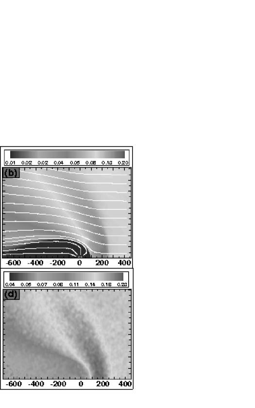
Figure 2: (a) Proton temperature, (b) proton density, (c) neutral hydrogen temperature, and (d) neutral hydrogen density distributions for Model 1. The positions of the termination shock (TS), heliopause (HP), and bow shock (BS) are indicated in (a), and streamlines indicating the plasma flow direction are shown in (b). The distance scale is in AU.

In Figure 2, we display the temperature and density distributions for protons and neutral hydrogen in the heliosphere for Model 1. Panel 2a shows the locations of the heliospheric boundaries, and streamlines in panel 2b indicate the paths of protons in the model. The LISM plasma is heated at the bow shock (BS) and diverted around the heliosphere (see Fig. 2a-b). The tangential discontinuity of the heliopause (HP) separates the LISM plasma from the solar wind. In Model 1, the distances from the Sun to the HP and to the BS in the upwind direction are 100 AU and 260 AU, respectively. Inside the heliosphere, the cool, fast solar wind goes through a termination shock (TS), which is at 62 AU in Model 1. The solar wind is heated to temperatures in excess of $10^{6}$ K and diverted tailward. The neutral temperatures and densities are computed by taking moments of the particle distributions computed by the Boltzmann code (see Müller et al., 2000). In the region between HP and BS, the overdensity in neutral hydrogen referred to as the hydrogen wall is clearly visible in Figure 2d. Downwind of this hydrogen wall, neutral hydrogen is depleted but hot ($\approx 10^{5}$ K, see Fig. 2c). Note that if $\alpha>6$ then ${\rm M}<1$ (assuming ${\rm T}=8000$ K), in which case there will be no bow shock (Models 4–7). A more in-depth description of Models 1–10 and their properties will be provided in a future paper (Müller, Zank, & Wood 2000, in preparation).

The LISM protons are shock heated at the bow shock, and if there is no bow shock they are still heated by adiabatic compression at the heliopause. The interstellar neutrals are then heated by charge exchange with these protons, creating the high temperatures seen in Figure 2c. Charge exchange with outflowing solar wind protons also occurs, resulting in a flux of hot neutrals back through the heliopause and bow shock. Further charge exchanges can deposit additional energy both in the hydrogen wall and in front of the bow shock, and such processes can have measurable effects on the heliospheric structure (Zank et al., 1996). In general, higher heliospheric hydrogen temperatures and densities are observed for models with lower values of $\alpha$, which is not surprising since a lower $\alpha$ corresponds with a higher Mach number for the inflowing LISM and therefore more heating. Because higher temperatures and column densities will produce broader Lyman-$\alpha$ absorption profiles, models with higher Mach numbers will also generally produce more absorption.

The Boltzmann models provide us with velocity distributions throughout the heliosphere that we can use to compute the absorption profiles. In Figure 3, radial velocity distributions are displayed for neutral hydrogen particles in the upwind and downwind directions for Model 1. In order to create these distributions, particles are summed within $100\times 100$ AU boxes centered on the locations indicated in the figure. Poissonian error bars ($N^{0.5}$) are displayed for each velocity bin. The bin size of the histogram is 6 km s^-1. Gaussians have been fitted to the distributions (dashed lines), and the poor fits illustrate the non-Maxwellian character of the distributions.

The complexity of the distributions is due in part to the fact that the neutral particles are created by charge exchange with protons throughout the heliosphere with very different temperatures and flow velocities. The main peak consists mostly of neutral particles created by charge exchange with heated LISM protons in the hydrogen wall. Following the nomenclature used in Zank et al. (1996), these are called “component 1” neutrals. The distributions also contain some particles created by charge exchange with the very hot, decelerated solar wind protons in between the termination shock and heliopause, which for the upwind case in Figure 3 are seen after flowing back across the heliopause. These particles, the “component 2” neutrals, are particularly prevalent in the far wings of the distributions. The component 2 neutrals are far more abundant in downwind directions, explaining why the downwind distribution is broader and has more extended wings than the upwind distribution. Finally, there are a few particles in the distributions created by charge exchange with solar wind protons near the Sun, thereby creating a small population of neutrals with speeds of about $+400$ km s^-1 (see Fig. 3), which are referred to as “component 3” neutrals. At the upwind location shown in Figure 3, the peak of the distribution lies at about $-16$ km s^-1, which represents a significant deceleration from the $-26$ km s^-1 speed of the undisturbed LISM. At the downwind location shown in the figure, the average speed is about $+28$ km s^-1, slightly faster than the $+26$ km s^-1 LISM flow speed.

In Figure 4, we show the H I Lyman-$\alpha$ absorption predicted by Model 1 for an upwind and downwind line of sight. In computing such absorption profiles, we first divide the radial path through the heliosphere into many segments. We assign an H I density to each segment based on the number of particles found within a $4\times 5$ AU box containing the segment. To get viable statistics for the distribution of radial velocities for the segment, we must use a larger area of influence to determine the distribution histogram. We use a circle with a radius of 30 AU containing the segment for this purpose.

Velocities can be linearly mapped onto wavelengths using the familiar relation

$$\lambda=\lambda_{0}\left(1-\frac{v}{c}\right)^{-1},$$ (1)

where $\lambda_{0}=1215.6701$ Å is the rest wavelength of Lyman-$\alpha$. Thus, the velocity distribution defines a line profile function, $\phi_{\lambda}$, which is normalized so that

$$\int^{\infty}_{0}\phi_{\lambda}d\lambda=1.$$ (2)

The opacity profile in frequency space is (in cgs units)

$$\tau_{\nu}=0.02654fN\phi_{\nu},$$ (3)

where $f$ is the oscillator absorption strength and $N$ is the column density (i.e., the density times the pathlength of the line segment in question). For Lyman-$\alpha$, $f=0.4164$ (Morton, 1991). Since $\phi_{\nu}=(\lambda^{2}/c)\phi_{\lambda}$, the opacity profile in wavelength space is

$$\tau_{\lambda}=\frac{0.02654fN\lambda^{2}}{c}\phi_{\lambda}.$$ (4)

We compute these opacity profiles for each segment of the line of sight and then add them all up. The absorption profile is then simply $I_{\lambda}=I_{0}\exp(-\tau_{\lambda})$, where $I_{0}$ is the assumed background Lyman-$\alpha$ flux. In Figure 4, we simply assume $I_{0}=1$ for all wavelengths.

In the procedure described above, we have assumed that the line profile is regulated solely by Doppler motions. This is a very good approximation here since the velocity distributions are much broader than the core of the natural line broadening profile, and column densities are too low for the Lorentzian wings of the natural profile to become evident. We have also ignored the fine structure of Lyman-$\alpha$, but this has only a very minor effect since the two fine structure components are separated by only 1.3 km s^-1.

The H I properties displayed in Figures 2c-d were computed by taking moments of the velocity distribution functions. In Figure 4, we show absorption profiles computed directly from these moments (dashed lines). These profiles, however, are significantly different from those computed directly from the distributions, indicating that flow velocities and temperatures computed from moments do not define the characteristics of the distribution well enough to be used to accurately determine absorption profiles. Accurate absorption profiles can be computed only from the distributions themselves.

4 Comparing the Models with the Data

In Figures 5 and 6 we show the heliospheric absorption predicted for the lines of sight observed by HST for Models 1–7. The heliospheric absorption is combined with the LISM absorption (dotted lines) and then convolved with the instrumental line spread function before being plotted. For the sake of clarity, we display four of the models in Figure 5 and four in Figure 6, with Model 4 being shown in both. We have zoomed in on the red side of the absorption profiles since that is where most of the heliospheric absorption is located, astrospheric absorption being the more likely explanation for any excess absorption on the blue side (see §2).

The models certainly have no trouble producing observable absorption. In fact, the models tend to predict too much absorption, especially downwind. This downwind discrepancy may be even more dramatic than the figures suggest, because our models only extend 1000 AU in that direction, which may be far enough for lines of sight with $\theta\leq 125^{\circ}$ but is probably not far enough to incorporate all the heliospheric H I further downwind. Thus, we will underestimate the amount of heliospheric absorption toward Sirius and $\epsilon$ Eri.

The absorption exhibits some interesting nonlinear behavior, which is particularly pronounced in the downwind direction. As expected, the amount of absorption decreases with increasing $\alpha$ between $\alpha=2$ and $\alpha=5$, but the absorption increases between $\alpha=5$ and $\alpha=9.6$ before decreasing once again between $\alpha=9.6$ and $\alpha=18$ (see, e.g., the $\epsilon$ Eri panels of Figs. 5-6). Similar behavior is observed upwind, although it is not as dramatic. The transition between decreasing absorption and increasing absorption at $\alpha=5$ is presumably associated with the boundary between a supersonic and a subsonic LISM wind, which is at $\alpha=6$.

Unfortunately, none of the models does a very good job in reproducing the observations. Some of the apparent disagreement is illusory, however, because it can be fixed by tweaking either the assumed stellar Lyman-$\alpha$ profile or the assumed LISM absorption, or both.

In Figure 7, we show how this is done for two examples: the $\alpha=2.0$ model for the 36 Oph line of sight and the $\alpha=12.5$ model for the 31 Com line of sight. In both cases, we allow the assumed LISM absorption parameters to be altered within the uncertainties derived in the initial analyses of these data, which are determined partially from the analyses of other LISM lines (Dring et al., 1997; Wood et al., 2000). We also alter the shapes of the assumed stellar profiles to try to make the models fit the data (solid lines: original, dashed lines: altered profiles).

However, there are limits to the shapes a reasonable profile can have. This is especially true for 31 Com. The 31 Com Lyman-$\alpha$ emission line is very broad, meaning we cannot allow the slope of the line to become very large within the absorption region. This limits how effective profile changes are in helping us to force the heliospheric absorption model to fit the data. The narrower 36 Oph emission line allows us more leeway in altering the assumed profile. Thus, the changes from the original profiles to the new profiles in Figure 7 are much larger for 36 Oph than for 31 Com.

Another problem for 31 Com is that there is no evidence for excess absorption on the blue side of the line that would suggest the presence of astrospheric absorption, meaning that we cannot completely ignore the quality of fit on that side of the line, in contrast with the 36 Oph example. The quality of the 31 Com fit in Figure 7 is noticeably worse than that of the simpler LISM-only fit in Figure 1. Nevertheless, we conclude that the 31 Com fit in Figure 7 is just good enough to claim that the $\alpha=12.5$ model (Model 6) is barely consistent with the 31 Com observations at $\theta=73^{\circ}$. Based on Figure 7, we also claim that the $\alpha=2.0$ model (Model 1) is consistent with the 36 Oph observations at $\theta=12^{\circ}$.

We have performed an analysis like that in Figure 7 for all combinations of models and data, and in Figure 8 we show the best fits that can be obtained by such alterations of stellar profile and LISM absorption for Models 1–7. Many of the models that did not appear to agree well with the data in Figures 5–6 do fit the data well in Figure 8, but many still do not. In general, discrepancies near the base of the absorption (e.g., at $15<v<25$ km s^-1 for $\alpha$ Cen) are much harder to remedy than discrepancies farther in the wing of the absorption (e.g., at $v>25$ km s^-1 for $\alpha$ Cen). Large discrepancies near the base can generally only be fixed by introducing unreasonable fine structure into the assumed stellar Lyman-$\alpha$ profile.

Based on the results displayed in Figure 8, we provide in Table 1 our evaluation of which observed lines of sight are inconsistent with which models. None of the models discussed to this point (Models 1–7) are consistent with every line of sight. The low $\alpha$ models do better upwind and the high $\alpha$ models do better downwind. In general, the problem with the models that do not fit the data is that they predict too much absorption, the exception being the 36 Oph line of sight for which most of the models predict too little absorption. Model 7 is the only model that does not predict way too much absorption along the downwind line of sight to $\epsilon$ Eri.

For Models 8 and 9 in Table 1, we repeated the $\alpha=2.0$ model but with a lower LISM proton density and temperature, respectively, in order to see what effect this has on the predicted absorption (see §3). The n(H⁺) and T values assumed for these models are not the most likely values based on our current understanding of the LISM, but are still within the realm of possibility (see Table 1). Figure 9 compares the absorption predicted by all the $\alpha=2.0$ models. The figure shows that lowering the proton density decreases the amount of absorption downwind but has little effect elsewhere. Decreasing the temperature decreases the amount of absorption in all directions.

The changes in absorption indicated in Figure 9 are fairly modest, however, and certainly not enough to change the results shown in Figure 8, which suggest that $\alpha=2.0$ models are consistent only with the 36 Oph line of sight. If lower proton densities and/or temperatures were assumed for the models with other assumed $\alpha$’s, it might allow some of them to become consistent with some of the observed lines of sight. The $\alpha=12.5$ model could be made consistent with the $\epsilon$ Eri data, for example (see Fig. 8), but it would worsen the disagreement with the 36 Oph data.

Thus, we conclude that small changes in n(H⁺) and T will not solve the overall disagreement between the current Boltzmann models and the data. The models predict too much absorption downwind and sidewind relative to the amount of absorption observed upwind. Given the non-linear response of heliospheric models to different boundary conditions, we cannot completely exclude better agreement between data and models in another area of parameter space, perhaps one where the solar wind parameters are different than those that we assume. Moreover, barring unaccounted systematic errors in the assumed stellar profiles and the ISM absorption component, the heliospheric models employed in this study do not yet include all possibilities of interaction in the heliosphere. All of the models neglect the magnetic fields of both the solar wind and interstellar medium, the latter being very poorly constrained observationally. The Boltzmann kinetic models neglect neutral-neutral collisions, as well as proton-neutral collisions that are not accompanied by charge exchange, and neutral depletion due to photoionization close to the Sun.

Ironically, the one model listed in Table 1 that is consistent with all lines of sight is the four-fluid model (Model 10), which uses a less sophisticated treatment of the heliospheric H I than the Boltzmann models. Figure 10 shows the comparison of predicted and observed absorption for Model 10, both before and after the assumed stellar profile and ISM parameters are tweaked to maximize the quality of fit (as was done in Fig. 8 for Models 1–7). The agreement is good enough to claim that the model is consistent with all six lines of sight. Note that the absorption predicted by the four-fluid Model 10 is vastly different from that predicted by the Boltzmann Model 1 (see Fig. 10 and $\alpha=2.0$ model in Fig. 5), despite the fact that their input parameters are identical (see Table 1). This illustrates just how sensitive the predicted absorption is to how the H I velocity distributions are treated in the models.

There are several ways to interpret the results illustrated in Figure 10. It should be understood that the four-fluid model and the Boltzmann/kinetic models represent somewhat different physics for the neutral H distributions. The underlying assumption inherent in the four-fluid model is that some scattering of neutral H is present to ensure that the distributions of the individual components, if not the full distribution, is approximately Maxwellian. This process is absent in the kinetic models (see Zank et al. 1996 and Williams et al. 1997 for discussions concerning the four-fluid model assumptions). Figure 10 indicates that a good fit to the Lyman-$\alpha$ data along the six sightlines requires that the heliospheric neutral H distribution be very like that produced by the four-fluid model. That Boltzmann Model 1 and the four-fluid Model 10 produce quite different absorption profiles suggests the possibility that additional physical processes with respect to H may need to be incorporated in the Boltzmann codes. Unfortunately, we have not yet explored parameter space in sufficient detail to rule out the possibility that a Boltzmann model does in fact exist that results in acceptable agreement with the Lyman-$\alpha$ data, assuming reasonable input parameters. In addition, other factors not included, explicitly or implicitly, in either the Boltzmann or four-fluid models (such as magnetic fields) may still be required to fully address these issues.

5 Summary

We have compared H I Lyman-$\alpha$ absorption profiles computed using fully self-consistent kinetic/hydrodynamic models of the heliosphere with profiles observed in UV spectra obtained by HST. We make this comparison for six different lines of sight through the heliosphere toward six nearby stars. Our results are summarized as follows:

1.

Most of our models use a Boltzmann particle code for the neutrals, allowing us to estimate neutral velocity distributions throughout the heliosphere. These velocity distributions are far from Maxwellian, having extended wings that lead to broad Lyman-$\alpha$ absorption profiles.

2.

Average temperatures and flow velocities can be computed by taking moments of the velocity distributions, and Lyman-$\alpha$ absorption profiles can be computed from these moments. However, we find that such profiles do not generally agree well with more accurate profiles computed directly from the distributions. Thus, the moments of the distributions apparently do not provide enough information about their shapes to yield accurate absorption profiles.

3.

The amount of absorption predicted by the models generally increases as the assumed Mach number of the interstellar wind is increased (i.e., the $\alpha$ parameter is decreased). However, there are some interesting non-linear effects near the transition between subsonic and supersonic models (i.e., near $M=1$).

4.

The Boltzmann models tend to predict too much absorption in sidewind and downwind directions, and too little absorption upwind. This problem is exacerbated at higher Mach numbers. Varying the assumed interstellar temperature and proton density does not seem to help.

5.

In contrast to the Boltzmann models, a four-fluid model that uses a less sophisticated, multi-fluid treatment of the neutrals is consistent with the data. The absorption predicted by this model is very different from that predicted by a Boltzmann model with the same input parameters, emphasizing how crucial the treatment of the neutrals is for accurately predicting Lyman-$\alpha$ absorption profiles.

6.

Possible reasons for the lack of success for the Boltzmann models in reproducing the data include the neglect of collisions not involving charge exchange in those models, or perhaps an insufficient exploration of parameter space. There may also be other physical processes that have not been considered in either the Boltzmann or four-fluid models which could be important and affect our results, such as processes involving magnetic fields.

Table 1: Model Parameters

Model #	Code	n(H+)	T	$\alpha$	M	Consistent with Data?
		(cm-3)	(K)			$\theta=12^{\circ}$	$52^{\circ}$	$73^{\circ}$	$112^{\circ}$	$139^{\circ}$	$148^{\circ}$
1	Boltzmann	0.10	8000	2.0	1.7	Y	N	N	N	N	N
2	Boltzmann	0.10	8000	3.5	1.3	Y	N	N	N	N	N
3	Boltzmann	0.10	8000	5.0	1.1	N	Y	Y	N	N	N
4	Boltzmann	0.10	8000	7.6	0.9	N	Y	Y	N	N	N
5	Boltzmann	0.10	8000	9.6	0.8	N	Y	N	N	N	N
6	Boltzmann	0.10	8000	12.5	0.7	N	Y	Y	Y	Y	N
7	Boltzmann	0.10	8000	18.0	0.6	N	Y	Y	Y	Y	Y
8	Boltzmann	0.05	8000	2.0	1.7	Y	N	N	N	N	N
9	Boltzmann	0.10	6000	2.0	2.0	Y	N	N	N	N	N
10	Four-fluid	0.10	8000	2.0	1.7	Y	Y	Y	Y	Y	Y

Figure 1: HST Lyman-$\alpha$ spectra of six stars, with the six lines of sight sampling different angles ($\theta$) relative to the upwind direction of the interstellar flow into the heliosphere. Very broad H I absorption is easily apparent in all the data, as is much narrower deuterium absorption about $-80$ km s^-1 from the H I absorption. Each panel shows the assumed stellar profile (solid line) and interstellar absorption (dotted line), as determined from previously published work (see text). In many cases, the interstellar absorption does not account for all of the observed absorption, presumably indicating the presence of heliospheric and/or astrospheric absorption.

Figure 3: H I radial velocity distributions for two different heliospheric locations based on Model 1, where $\theta$ is the angle relative to the upwind direction of the interstellar flow into the heliosphere, and R is the distance from the Sun. The dashed lines are Gaussian fits to the distributions, and residuals of the fits are shown below each panel. The poor quality of the fits illustrates the non-Maxwellian character of the distributions.

Figure 4: H I Lyman-$\alpha$ absorption profiles for upwind ($\theta=0^{\circ}$) and downwind ($\theta=180^{\circ}$) lines of sight, computed for Model 1. The dashed lines are profiles computed from temperatures and flow velocities calculated by taking moments of the velocity distributions, while the histograms are profiles computed directly from the distributions themselves. The disagreement between the two demonstrates the importance of calculating absorption profiles directly from the distributions.

Figure 5: A reproduction of Fig. 1, zoomed in on the red side of the H I absorption line, where we also show the absorption predicted by Models 1–4, which assume $\alpha=2.0-7.6$.

Figure 6: Same as Fig. 5, but for subsonic Models 4–7, which assume $\alpha=7.6-18.0$.

Figure 7: Two examples of how models that do not appear to fit the data well in Figs. 5–6 can be made to fit the data by altering the assumed stellar Lyman-$\alpha$ profile and/or tweaking the assumed interstellar absorption parameters within the uncertainties determined from previously published analyses. The dashed lines are the original stellar profiles, and the thin solid lines are the new ones. In each panel, the dotted line represents the assumed interstellar absorption, and the thick solid line is the combination of the interstellar and heliospheric absorption for the model indicated in the figure, which in both cases fits the data reasonably well.

Figure 8: As suggested by Fig. 7, agreement between the models and observations can be greatly improved by tweaking the assumed stellar Lyman-$\alpha$ line and/or ISM absorption. This figure shows the best possible fits that can be obtained after doing this for all the models (Models 1–7) and lines of sight shown in Figs. 5–6. This procedure results in good agreement with the data in some instances, but substantial disagreement remains in most cases.

Figure 9: Comparison of the H I absorption predicted by the three $\alpha=2.0$ Boltzmann models listed in Table 1, indicating the degree to which the absorption is decreased by reducing the assumed interstellar proton density (Model 8) and temperature (Model 9).

Figure 10: Comparison of the H I absorption predicted by the $\alpha=2.0$ four-fluid model listed in Table 1 (Model 10) and the observations, both before (thin dashed line) and after (thick dashed line) the assumed stellar line profile and ISM absorption are tweaked to maximize the agreement with the data. Reasonably good agreement is observed for all six lines of sight.

References

- Baranov, Izmodenov, & Malama (1998) Baranov, V. B., Izmodenov, V. V., & Malama, Y. G. 1998, J. Geophys. Res., 103, 9575
- Baranov & Malama (1993) Baranov, V. B., & Malama, Y. G. 1993, J. Geophys. Res., 98, 15157
- Baranov & Malama (1995) Baranov, V. B., & Malama, Y. G. 1995, J. Geophys. Res., 100, 14755
- Bertin et al. (1995b) Bertin, P., Lamers, H. J. G. L. M., Vidal-Madjar, A., Ferlet, R., & Lallement, R. 1995b, A&A, 302, 899
- Bertin et al. (1995a) Bertin, P., Vidal-Madjar, A., Lallement, R., Ferlet, R., & Lemoine, M. 1995a, A&A, 302, 889
- Burlaga et al. (1994) Burlaga, L. F., Ness, N. F., Belcher, J. W., Szabo, A., Isenberg, P. A., & Lee, M. 1994, J. Geophys. Res., 99, 21511
- Dring et al. (1997) Dring, A. R., Linsky, J., Murthy, J., Henry, R. C., Moos, W., Vidal-Madjar, A., Audouze, J., & Landsman, W. 1997, ApJ, 488, 760
- Fisk, Kozlovsky, & Ramaty (1974) Fisk, L. A., Kozlovsky, B., & Ramaty, R. 1974, ApJ, 190, L35
- Gayley et al. (1997) Gayley, K. G., Zank, G. P., Pauls, H. L., Frisch, P. C., & Welty, D. E. 1997, ApJ, 487, 259
- Gloeckler et al. (1993) Gloeckler, G., et al. 1993, Science, 261, 70
- Gloeckler et al. (1994) Gloeckler, G., et al. 1994, J. Geophys. Res., 99, 17637
- Holzer (1989) Holzer, T. E. 1989, ARA&A, 27, 199
- Izmodenov, Lallement, & Malama (1999) Izmodenov, V. V., Lallement, R., & Malama, Y. G. 1999, A&A, 342, L13
- Klecker (1995) Klecker, B. 1995, Space Sci. Rev., 72, 419
- Lallement et al. (1995) Lallement, R., Ferlet, R., Lagrange, A. M., Lemoine, M., & Vidal-Madjar, A. 1995, A&A, 304, 461
- Linsky et al. (1993) Linsky, J. L., Brown, A., Gayley, K., Diplas, A., Savage, B. D., Ayres, T. R., Landsman, W., Shore, S. N., & Heap, S. R. 1993, ApJ, 402, 694
- Linsky et al. (2000) Linsky, J. L., Redfield, S., Wood, B. E., & Piskunov, N. 2000, ApJ, 528, 756
- Linsky & Wood (1996) Linsky, J. L., & Wood, B. E. 1996, ApJ, 463, 254
- Linsky (1998) Linsky, J. L. 1998, Space Sci. Rev., 84, 285