The Infall Region of Abell 576:
Independent Mass and Light Profiles

Abstract

We describe observations of the nearby ($cz=11,487~{}{\rm km~{}s}^{-1}$) cluster of galaxies Abell 576 beyond the virial radius and into the infall region where galaxies are on their first or second pass through the cluster. Using 1057 redshifts, we use the infall pattern in redshift space to determine the mass profile of A576 to a radius of $\sim 4~{}h^{-1}{\rm Mpc}$. This mass estimation technique makes no assumptions about the equilibrium state of the cluster. Within $\sim 1~{}h^{-1}{\rm Mpc}$, the mass profile we derive exceeds that determined from X-ray observations by a factor of $\sim 2.5$. At $\sim 2.5~{}h^{-1}{\rm Mpc}$, however, the mass profile agrees with virial mass estimates. Our mass profile is consistent with a Navarro, Frenk, & White (1997) or Hernquist (1990) profile, but it is inconsistent with an isothermal sphere.

R-band images of a $3^{\circ}\times 3^{\circ}$ region centered on the cluster allow an independent determination of the cluster light profile. We calculate the integrated mass-to-light ratio as a function of cluster radius; it decreases smoothly from the core to $M/L_{R}\sim 300h$ at $\sim 4~{}h^{-1}{\rm Mpc}$. The differential $M/L_{R}$ profile decreases more steeply; we find $\delta M/\delta L_{R}\sim 100h$ at $\sim 4~{}h^{-1}{\rm Mpc}$, in good agreement with the mass-to-light ratios of individual galaxies. If the behavior of $M/L_{R}$ in A576 is general, $\Omega_{m}\lesssim 0.4$ at 95% confidence.

For a Hernquist model, the best-fit mass profiles differ from the observed surface number density of galaxies; the galaxies have a larger scale radius than the mass. This result is consistent with the centrally peaked $M/L_{R}$ profile. Similarly, the scale radius of the light profile is larger than that of the mass profile. We discuss some potential systematic effects; none can easily reconcile our results with a constant mass-to-light ratio.

1 Introduction

Clusters of galaxies are important probes of the distribution of both matter and light on intermediate scales ($0.1-10~{}h^{-1}{\rm Mpc}$). They are also interesting laboratories for studying the effects of local environment on cluster galaxies. Most studies of clusters concentrate on the central regions where the cluster is probably in equilibrium. Studies of the galaxy distribution on larger scales tend to focus either on general properties of large-scale structure (e.g., deLapparent, Geller, & Huchra (1986); Dressler et al. (1987)) or on individual superclusters (e.g., Giovanelli & Haynes 1985). There are relatively few examinations (Regös & Geller (1989); Lilje & Lahav (1991); van Haarlem et al. (1993); van Haarlem & van de Weygaert (1993); Praton & Schneider (1994); Diaferio & Geller (1997); Vedel & Hartwick (1998); Ellingson et al. (1999)) of the infall regions of clusters. In these regions, the galaxies are falling into the gravitational potential well of the cluster, but they have not yet reached equilibrium. Many, perhaps most, of the galaxies in this region are on their first orbit of the cluster. They populate a regime between that of relaxed cluster cores and the surrounding large-scale structure where the transition from linear to non-linear clustering occurs.

Here we use 1057 redshifts and photometry of 2118 galaxies in the infall region of Abell 576 ($cz=11,487~{}{\rm km~{}s}^{-1}$) to address an unresolved problem in astrophysics: the relative distribution of mass and light on large scales. Zwicky (1933; 1937) originally found that the mass of the Coma cluster greatly exceeds the sum of the masses of the stars. More recently, calculations of mass-to-light ratios for galaxy clusters yield values of several hundred in solar units (Dressler (1978); Faber & Gallagher (1979); Adami et al. 1998b ). Girardi et al. (2000) calculated mass-to-light ratios for a large sample of nearby clusters within the virial radius and obtained typical values of $M/L_{B_{j}}\sim 220-250h$ (all $M/L$ values are in solar units, i.e., $M_{\odot}/L_{\odot}$). David, Jones, & Forman (1995) find $M/L_{V}\sim 200-300h$ for seven groups and clusters using masses calculated from the observed X-ray emission, and the CNOC survey finds $M/L_{r}\sim 290\pm 60h$ for a sample of distant clusters (Carlberg et al. (1996)).

The mass density parameter $\Omega_{m}$ of the universe can be estimated by assuming that the universal mass-to-light ratio is equal to the ratio in rich clusters of galaxies (e.g., Carlberg et al. 1996). There have been few attempts to determine mass-to-light ratios directly at larger radii (Mohr & Wegner (1997); Small et al. (1998); Kaiser et al. (2000)), where clusters are in neither hydrostatic nor virial equilibrium. Neither X-ray observations nor virial analysis provide accurate mass determinations at these large radii. Two methods with particular promise are weak gravitational lensing (Kaiser et al. (2000)) and kinematics of the infall region (Diaferio & Geller 1997, hereafter DG; Diaferio 1999, hereafter D99). Kaiser et al. analyzed the weak lensing signal from a supercluster at $z\approx 0.4$ and found no significant evidence for variations in mass-to-light ratios on scales less than $\sim 6~{}h^{-1}{\rm Mpc}$. Metzler et al. (1999), however, show that lensing by intervening filamentary structures probably associated with clusters can result in significant overestimates of cluster masses. Geller, Diaferio, & Kurtz (1999, hereafter GDK) applied the kinematic method of DG to the infall region of the Coma cluster. They successfully reproduced the X-ray derived mass profile and extended direct determinations of the mass profile to $\sim 10~{}h^{-1}{\rm Mpc}$. Adequate photometric data necessary to compute the mass-to-light profile for this large region around Coma are not yet available.

Here we apply the method of DG to A576. In redshift space, the infall regions of clusters form a characteristic trumpet-shaped pattern. These caustics arise because galaxies fall into the cluster as the cluster potential overwhelms the Hubble flow (Kaiser (1987); Regös & Geller (1989)). Under simple spherical infall, the galaxy phase space density becomes infinite at the caustics. DG analyzed the dynamics of infall regions with numerical simulations and found that in the outskirts of clusters, random motions due to substructure and non-radial motions make a substantial contribution to the amplitude of the caustics which delineate the infall regions. DG showed that the amplitude of the caustics is a measure of the escape velocity from the cluster; identification of the caustics therefore allows a determination of the mass profile of the cluster on scales $\lesssim 10h^{-1}{\rm Mpc}$.

DG show that nonparametric measurements of caustics would yield cluster mass profiles accurate to $\sim$30% on scales $1-10~{}h^{-1}{\rm Mpc}$, if (1) the redshift space coordinates of the dark matter particles were measurable, and (2) the cluster mass within the virial radius were known exactly. More realistically, by using simulated catalogs of galaxies formed and evolved using semi-analytic procedures within the dark matter halos of dissipationless N-body simulations (Kauffmann et al. 1999a ), D99 shows that the identification of caustics in the realistic redshift diagrams of clusters recovers their mass profiles within a factor of 2 to several Megaparsecs from the cluster center without a separate determination of the central mass. When combined with wide-field photometry, this approach allows a determination of the mass-to-light ratio on large scales which is independent of the assumption that light traces mass. This method assumes only that galaxies trace the velocity field. Indeed, simulations suggest that velocity bias, if any, is very weak on both linear and non-linear scales (Kauffmann et al. 1999a ; Diaferio et al. (1999)). Vedel & Hartwick (1998) used simulations to explore an alternative parametric maximum likelihood analysis of the infall region. Their technique requires assumptions about the functional forms of the density profile and the velocity dispersion profile.

Here, we analyze the caustics within a $\sim 4~{}h^{-1}{\rm Mpc}$ radius to determine the mass profile of Abell 576, an Abell richness class 1 cluster (Abell (1958)) at a redshift of $z=0.0383$. Mohr et al. (1996, hereafter M96) extensively studied the inner square degree of this cluster. Using photometric observations of a $3^{\circ}\times 3^{\circ}$ region centered on the cluster, we determine the mass-to-light profile within this range. The integrated mass-to-light ratio smoothly decreases with radius out to $\sim 4~{}h^{-1}{\rm Mpc}$. Remarkably, the differential mass-to-light ratio decreases steeply to values typical of individual galaxy halos.

We describe the photometric and spectroscopic observations in $\S$ 2. In $\S$ 3, we determine the amplitude of the caustics and calculate the mass profile. We analyze the X-ray observations in $\S$ 4 and compare the X-ray mass profile to the infall mass profile. We discuss the contribution of background galaxies in $\S$ 5. We determine the surface number density profile in $\S$ 6 and compare it to the mass distribution. We test for luminosity segregation in $\S$ 7 and calculate the light profile in $\S$ 8. We compare the mass and light profiles of the cluster in $\S 9$. We discuss possible systematic effects in $\S 10$ and conclude in $\S 11$.

2 Data

2.1 Images

We obtained ten 200-second R-band images of A576 with the MOSAIC camera on the 0.9-m telescope at Kitt Peak on 1999 February 13-14; both nights were photometric. The MOSAIC camera consists of 8 CCD chips, each with a field of view of 15${}^{\prime}\times 30^{\prime}$. Our mosaic thus covers approximately a $3^{\circ}\times 3^{\circ}$ region centered on A576. Adjacent images overlap by 1$\farcm$0. We imaged the central square degree on both nights; the 14 February image is offset 1$\farcm$0 N and 1$\farcm$0 E from the 13 February image. We reduced the images using standard IRAF procedures in the mscred package. We use SExtractor (Bertin & Arnouts (1996)) to locate sources in the images and calculate magnitudes. SExtractor divides the image into segments and assigns pixels to individual objects to deal with crowded images. Analysis of simulated CCD images show that SExtractor accurately recovers total magnitudes of faint galaxies (Bertin & Arnouts (1996)). We use the MAG_BEST magnitudes, which are equivalent to MAG_AUTO, an aperture magnitude, unless an object has one or more close neighbors likely to contaminate the flux by more than 10%, in which case MAG_BEST=MAG_ISOC, an isophotal magnitude with a correction based on a Gaussian light profile. We classify all objects with CLASS_STAR$<$ 0.6 as galaxy candidates; we then visually inspect these to eliminate binary stars and artifacts. We calibrate the photometry with observations of M67 (Chevalier & Ilovaisky (1991); Anupama et al. (1994)) and Landolt (1992) fields. We obtain the color correction term from the data set for the entire observing run and the extinction coefficient from fits to data on all chips for each night. To allow for possible chip-to-chip sensitivity variations, we calculate the zero point separately for each chip (Brown et al. (2000)).

We use the IRAF package apphot to test the accuracy of the SExtractor magnitudes. Using curves of growth on the images of a few dozen galaxies covering the range of magnitudes $m_{R}=14$ to $m_{R}$ = 18, we estimate their total magnitudes within large apertures (50-150^′′). We find excellent agreement ($\lesssim 0.1$ mag) between the IRAF total aperture magnitudes and the SExtractor MAG_BEST magnitudes.

We restrict our analyses to objects with MAG_BEST$<$18.0, approximately the limit of the classification. We use the offset images of the central region to estimate the consistency of our magnitudes; the distribution of $m_{2}-m_{1}$ ($m_{1}$ and $m_{2}$ are the magnitudes calculated from the first and second night respectively) for galaxies with $m_{R}<$18.0 is well represented by a Gaussian with a zero point difference of -0.002 mag and $\sigma_{(m_{2}-m_{1})}\approx 0.09$ mag. The scatter in the magnitude determination increases significantly with apparent magnitude (Figure 1). We thus estimate that our magnitudes are internally consistent to about 0.06 mag ($\sigma_{m_{1}}^{2}\approx\sigma_{m_{2}}^{2}\approx{\sigma_{(m_{2}-m_{1})}}^{2}/2$). In Table 1, we list the R band magnitudes and their uncertainties (quadrature sums of the internal SExtractor errors and the 0.06 mag scatter from galaxies with multiple observations) for galaxies with redshifts from FLWO ($\S 2.2$). We also include estimates of Galactic extinction in the R band ($A_{R}$) based on the dust maps of Schlegel, Finkbeiner, & Davis (1998). Mohr et al. (2000) will list redshifts collected by JJM and GW. Magnitudes for these galaxies as well as those without redshifts are available upon request from the authors. In the entire survey region, we identify 825 and 2118 galaxies with $m_{R}<$17.0 and $m_{R}<$18.0 respectively.

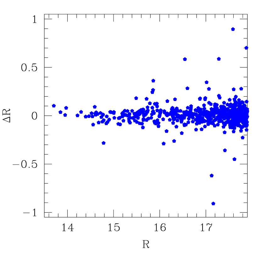
Figure 2: (a) Comparison of our MAG_BEST magnitudes with those of M96. Our magnitudes are systematically brighter. (b) Comparison of our magnitudes with those of M96 after processing both data sets with SExtractor.

We compare our photometry with that of M96. Figure 2a shows the difference in magnitude between the two studies as a function of our magnitudes. The comparison suggests that our magnitudes are systematically brighter by $\sim 0.1$ mag. Further analysis, however, shows that the differences between our magnitudes and M96 can be attributed to differences in the reduction packages (SExtractor versus FOCAS). For example, FOCAS uses a global estimate of background counts while SExtractor uses a local estimate. A complete comparison of the differences between these packages is beyond the scope of this work. A reanalysis of the M96 data using SExtractor produces excellent agreement (Figure 2b) between the two independent photometric data sets (Mohr et al. (2000)).

Out of 823 galaxies with redshifts selected without reference to these images ($\S 2.2$), SExtractor misses 28. Visual inspection reveals that 17 of these galaxies are in the halos of bright stars; the rest lie in chip gaps. For the 17 galaxies in stellar halos, we perform photometry with apphot. Unfortunately, three of these galaxies are located within $\sim 1^{\prime}.5$ of the X-ray center of the cluster (a saturated star is $1^{\prime}.1$ from the X-ray center), which increases the uncertainty of the central light. We make no correction for the regions of sky covered by saturated stars; this approach may lead to a slight underestimate in the light profile.

2.2 Spectroscopy

We used the FAST spectrograph (Fabricant et al. (1998)) on the 1.5-m Tillinghast telescope of the Fred Lawrence Whipple Observatory (FLWO) to obtain 529 spectra of galaxies within $4^{\circ}$ ($\approx 8~{}h^{-1}{\rm Mpc}$) of the center of A576. FAST is a long-slit spectrograph with a CCD detector. Integration times were typically 4-20 minutes, with spectral resolution of 6-8 Å. We analyzed the spectra at the Telescope Data Center at the Smithsonian Astrophysical Observatory using the xcsao and emsao tasks, which are standard cross-correlation fitting routines (Kurtz & Mink (1998)) available in the IRAF package r2rvsao. In this technique, template galaxy spectra are cross-correlated with the observed log-wavelength binned spectra to determine the redshift which provides the best fit for a particular template. Cross-correlation fits with R values of $\gtrsim 4.0$ are acceptable; most spectra have larger R values (the goodness of fit increases with R value).

We observed infall galaxy candidates in two campaigns; these occurred before and after obtaining the MOSAIC images described above. To select candidates for the first campaign (1999 January-February), we obtained galaxy positions from digital scans of the POSS I plates, using a method developed by Daniel Koranyi (1999) to discriminate between stars and galaxies. We extracted sources from the plate scans with SExtractor. We included all objects with staricity parameter $<$0.6 and ISO7-to-ISO2 isophotal ratio greater than 0.25. Comparison with visual inspection suggests that $\lesssim 1\%$ of galaxies are misclassified as stars using this criterion. We visually inspected the remaining objects to eliminate stars from the sample. For galaxies with $m_{R}\lesssim 15.3$, we measured redshifts in magnitude order. Because the magnitude order was taken from the plate scans, this ordering is not strictly accurate, and we could not obtain redshifts for some low surface brightness galaxies. Out of 300 candidates, this campaign yielded 293 redshifts (11 candidates were stars, plate flaws, or unobservable; 4 galaxies were serendipitously observed).

In the second campaign (1999 October-2000 February), we selected candidates from the MOSAIC images. Prior to the second campaign, our redshift sample was $\sim 95\%$ complete for $m_{R}<15.3$. In the second campaign, we observed 236 galaxies in magnitude order as determined from the MOSAIC images. We list the redshifts and $m_{R}$ magnitudes of the galaxies from both campaigns in Table 1. Table 2 lists the positions and redshifts of galaxies outside the MOSAIC images.

Two of us (JJM and GW) obtained 528 redshifts of galaxies in the central $2^{\circ}\times 2^{\circ}$ of this region for a separate Jeans’ analysis of the central region of A576 (Mohr et al. (2000)). 281 of these redshifts are from M96; the remainder will be published in Mohr et al. (2000). These redshifts were measured at the Decaspec (Fabricant & Hertz (1990)) at the 2.4-m MDM telescope on Kitt Peak and Hydra, the multifiber spectrograph on the WIYN telescope on Kitt Peak. Figure 3 shows the fraction of galaxies with redshifts as a function of R-band magnitude. We divide the sample into the region mostly covered by JJM and GW (projected radius ${R_{p}<1^{\circ}}$) and the region mostly covered by this study (${R_{p}>1^{\circ}}$). Within the $3^{\circ}\times 3^{\circ}$ region covered by our images, the total sample of 817 galaxies is 100% (99.7%) complete to a limiting magnitude of $m_{R}=16.2(16.5)$; the latter is the completeness limit for the photometric region.

3 Galaxy Infall Method and the Mass Profile

We briefly review the method DG and D99 develop to estimate the mass profile of a galaxy cluster by identifying its caustics in redshift space. The method assumes that clusters form through hierarchical clustering and requires only galaxy redshifts and positions on the sky. The amplitude $\mathcal{A}\mathnormal{(}r)$ of the caustics is half of the distance between the upper and lower caustics in redshift space. Assuming spherical symmetry, $\mathcal{A}\mathnormal{(}r)$ is related to the cluster gravitational potential $\phi(r)$ by

$$\mathcal{A}\mathnormal{}2(r)=-2\phi(r)\frac{1-\beta(r)}{3-2\beta(r)}$$ (1)

where $\beta(r)$ is the velocity anisotropy parameter. DG show that the mass of a spherical shell of radii [$r_{0},r$] within the infall region is given by the integral of the square of the amplitude $\mathcal{A}\mathnormal{(}r)$

$$GM(<r)-GM(<r_{0})=F_{\beta}\int_{r_{0}}^{r}\mathcal{A}\mathnormal{}2(x)dx$$ (2)

where $F_{\beta}\approx 0.5$ is a filling factor with a numerical value estimated from simulations. Variations in $F_{\beta}$ lead to some systematic uncertainty in the derived mass profile. Our mass profile extends to $\sim 3r_{200}$ (the average density within $r_{\delta}$ is $\delta$ times the critical density, $\S 4.1$); within this radius, $F_{\beta}$ varies by $\lesssim 15\%$ in simulations (see D99 for a more detailed discussion).

Operationally, we identify the caustics as curves which delineate a significant drop in the phase space density of galaxies in the projected radius-redshift diagram. Galaxies outside the caustics are also outside the turnaround radius. For a spherically symmetric system, taking an azimuthal average amplifies the signal of the caustics in redshift space and smooths over small-scale substructures. D99 described this method in detail and showed that, when applied to simulated clusters with galaxies modelled with semi-analytic techniques, it recovers the actual mass profiles within a factor of 2 to 5-10$~{}h^{-1}{\rm Mpc}$ from the cluster center. D99 describes some potential systematic effects including projection effects and variation in the galaxy orbit distribution $\beta(R_{p})$.

Simulations are necessary to estimate the uncertainties due to projection effects and deviations from spherical symmetry. In the simulations of D99, the degree of definition of the caustics depends on the underlying cosmology; in simulations, caustics are better defined in a low-density universe than a closed, matter-dominated universe (D99). Surprisingly, the caustics of Coma, A576, and several other clusters (Rines et al. (2000)) are generally better defined than those of the simulated clusters. Thus, the uncertainties estimated from these simulations might be overestimates.

We apply the technique of D99 to our A576 survey to determine the spatial and velocity center of the region as well as the location of the caustics. In this technique, we determine the center of the system from a hierarchical cluster analysis. The center thus derived, $\alpha_{opt}=$ 7:21:31.96, $\delta_{opt}=$+55:45:20.6 (J2000), $cz=11,487~{}{\rm km~{}s}^{-1}$, lies 50^′′ ($28~{}h^{-1}{\rm kpc}$) from the X-ray center (M96, from Einstein IPC data; see also $\S$ 4 for ASCA data). Our measurement of the central velocity of the infall region agrees well with previous estimates (Struble & Rood 1991, M96).

Figure 4 shows the projected radius from the cluster center versus redshift for galaxies within $cz_{lim}=4000~{}{\rm km~{}s}^{-1}$ of the cluster center. This range of redshifts includes all galaxies which may be members of the infall region. Solid lines indicate the caustics determined using the method of D99 based on a multidimensional adaptive kernel method (Silverman (1986); Pisani (1993); Pisani (1996)). This technique has been applied to numerical simulations (D99) as well as to the Coma cluster (GDK). As discussed in D99, it is necessary to rescale $h_{v}$ and $h_{r}$, the velocity and radial smoothing lengths so that spherical smoothing windows can be used. With an appropriate choice of this scaling relation $q=h_{v}/h_{r}$, the location of the caustics should be insensitive to small changes in $q$. In our case, $q=25$ satisfies this criterion. Following D99, we define the caustic amplitude $\mathcal{A}\mathnormal{(}r)$ as the minimum of the upper and lower amplitude estimates. This prescription is identical to averaging the two estimates for an isolated, spherically symmetric system; taking the minimum reduces the sensitivity to massive substructure and contamination.

We note that in A576, the location of the caustics is sensitive to substructure at $1.5-2.2h^{-1}{\rm Mpc}$. The caustic amplitude decreases sharply to $\sim 800~{}{\rm km~{}s}^{-1}$ somewhere in this region, though the radius of the decrease is sensitive to the smoothing parameter $q$. Figure 5 shows the caustics determined by setting $q=10$, 25, and 50. Small values of $q\sim 10$ seem to oversmooth the caustics and the sharp decrease occurs at $\sim 2.2h^{-1}{\rm Mpc}$, whereas the sharp decrease occurs at $\sim 1.5h^{-1}{\rm Mpc}$ for larger values of $q=25-50$. The amplitude of the caustics is stable both at radii smaller than $\sim 1.5h^{-1}{\rm Mpc}$ and at radii larger than $\sim 2.2h^{-1}{\rm Mpc}$. D99 gives the prescription for estimating the uncertainties in the caustic amplitude; this prescription reflects the scatter due to projection effects in the simulations. We show these $1\sigma$ uncertainties in Figure 4.

We define membership of the infall region from the caustics; hereafter, galaxies outside these caustics are interlopers. Of the 497 galaxies within $cz_{lim}$ of the velocity center of A576, 368 are within the infall region. Figure 6 shows the distribution of these galaxies on the sky. There is a noticeable deficit of infalling galaxies NW of the cluster center.

3.1 Comparison of Mass Profile to Models

We compare our results to Navarro, Frenk, & White (1997, hereafter NFW ), Hernquist (1990), and singular isothermal sphere mass profiles. The Hernquist profile is an analytic form proposed as a model of elliptical galaxies and bulges (Hernquist 1990). The “universal density profile” of NFW accurately models the mass profiles of dark matter halos in a variety of cosmological simulations (NFW ). Other simulations suggest that the NFW profile may not be accurate at small radii (e.g., Moore et al. (1998)), but these differences are unimportant on the scales we probe here. These mass profiles are:

$$M_{NFW}(r)=C_{NFW}a[{\rm\ln}\Bigl{(}\frac{r+a}{a}\Bigr{)}-\frac{r}{r+a}],$$ (3)

$$M_{Hern}(r)=C_{Hern}\frac{ar^{2}}{(r+a)^{2}},$$ (4)

$$M_{iso}(r)=C_{iso}r$$ (5)

respectively, where $a$ is the characteristic radius and $C$ is a normalization factor. These forms of the mass profiles minimize the correlation between the parameters. For the Hernquist profile, the mass $M_{c}$ within $a$ is $C_{Hern}a/4$, and the total mass of the system is $M_{tot}=C_{Hern}a$. From Equation 2, a singular isothermal sphere mass profile produces caustics with constant amplitudes. However, Figure 4 shows that the amplitude of the caustics decreases with radius.

We fit these models to the observed mass profile by minimizing $\chi^{2}$; Table 3 lists the results. The measures of the cumulative mass profiles are not independent; thus, the values of $\chi^{2}$ are indicative and are only meaningful when compared with each other. The best-fit parameters are insensitive to the inclusion or exclusion of the three data points where the caustics are unstable ($1.5<R_{p}<2.2h^{-1}{\rm Mpc}$). Figure 7 shows the three profiles which best fit the infall mass profile and Figure 8 shows the mass density profile. The latter display has the benefit that the data points are largely indepedendent of one another. The density of the cluster varies by five orders of magnitude across our sample; the overall agreement between these profiles and the data is remarkable. The isothermal sphere profile is strongly excluded. The Hernquist profile yields a better $\chi^{2}$ than the NFW profile, but both are acceptable. This conclusion agrees with GDK, who found that the mass profile of Coma is much better described by an NFW profile than an isothermal sphere.

From the infall mass profile, we can derive the values of overdensity radii $r_{\delta}$ directly. The mass $M_{\delta}$ contained within the overdensity radius $r_{\delta}$ exceeds the critical density by a factor of $\delta$. Two of the most commonly used radii are $r_{200}$ and $r_{500}$. The values of these radii are usually determined indirectly. For instance, Carlberg et al. (1997, hereafter CYE) define $r_{200}$ using the velocity dispersion $\sigma$ of a cluster. Evrard, Metzler, & Navarro (1996) use simulations to calibrate a correlation between $r_{500}$ and the emission-weighted X-ray temperature $T_{X}$. We estimate $r_{500}=0.96\pm 0.05h^{-1}{\rm Mpc}$ and $r_{200}=1.42\pm 0.07h^{-1}{\rm Mpc}$. A576 has an emission-weighted temperature of $T_{X}=3.77$ keV (see $\S 5$), which yields an estimate of $r_{500}=0.76\pm 0.16h^{-1}{\rm Mpc}$ using the Evrard et al. estimator, in agreement with our result.

3.2 Velocity Dispersion Profile

Many recent papers analyze the velocity dispersion profiles of clusters (e.g., Fadda et al. (1996); den Hartog & Katgert (1996); M96). When combined with the galaxy number density profile in the Jeans equation, the velocity dispersion profile can provide an estimate of the mass profile; Mohr et al. (2000) will perform this analysis for A576. Figure 9 shows the velocity dispersion profile of A576 where we compute the dispersions in bins of 25 galaxies. We also display the cumulative projected velocity dispersion profile $\sigma_{p}(<R_{p})$ (calculated from all galaxies inside $R_{p}$). The profile is centrally peaked and would probably be classified as ’Peaked’ by den Hartog & Katgert (1996).

Several authors (Fadda et al. (1996); CYE) suggest that the velocity dispersion of a cluster is best estimated by the asymptotic value of the cumulative projected velocity dispersion. For A576, $\sigma_{p}(<R_{p})$ decreases monotonically with radius for $R_{p}\gtrsim 0.5h^{-1}{\rm Mpc}$, suggesting that an asymptotic value of $\sigma_{p}(<R_{p})$ may not exist. At the largest radius we study, $\sigma_{p}(<R_{p})\approx 800~{}{\rm km~{}s}^{-1}$. This velocity dispersion is significantly smaller than $\sigma_{p}=977^{+124}_{-96}~{}{\rm km~{}s}^{-1}$ (M96) or $\sigma_{p}=914^{+50}_{-38}~{}{\rm km~{}s}^{-1}$ (Girardi et al. 1998).

The CYE estimate of $r_{200}$ is sensitive to the definition of $\sigma_{p}$. We obtain $r_{200}=1.69\pm 0.17h^{-1}{\rm Mpc}$ using the M96 value of $\sigma_{p}$, 1.5$\sigma$ larger than our estimate of $r_{200}=1.42\pm 0.07h^{-1}{\rm Mpc}$ ($\S 3.1$). Taking the value of $\sigma_{p}(<R_{p})\approx 800~{}{\rm km~{}s}^{-1}$ from the limit of our survey, $r_{200}=1.36\pm 0.15h^{-1}{\rm Mpc}$, in agreement with our infall estimate. The sensitivity of the CYE estimator to the aperture used to measure $\sigma_{p}$ may affect many of the results from studies of CNOC clusters because the properties of the composite CNOC cluster depend on the estimates of $r_{200}$ for individual clusters.

Based on the infall mass profile, we can predict the velocity dispersion profile with an assumption about the distribution of galaxy orbits. We assume that orbits are isotropic at all radii ($\beta=0$), and calculate the velocity dispersion profiles for the Hernquist and NFW models (Hernquist (1990), Equation 10; NFW, Equation 3). These predicted velocity dispersion profiles agree with the observed profile (Figure 9). The largest differences are at the radii where the caustic amplitude is unstable. Without fitting any parameters, we find $\chi^{2}=42$ and 59 for 14 degrees of freedom for the Hernquist and NFW profiles respectively. This result provides a consistency check on the infall mass profile and confirms that a Hernquist profile models the data better than an NFW profile.

3.3 Alternative Kinematic Mass Estimators

The two most commonly used kinematic mass estimators for clusters are the virial mass estimator and the projected mass estimator (Heisler, Tremaine, & Bahcall (1985)). These estimators both assume that clusters are relaxed systems. Numerical simulations, however, suggest that both of these mass estimators typically overestimate the true mass profile of a relaxed cluster by $\sim 20\%$ (Aceves & Perea (1999)).

If clusters are not relaxed, these estimators may provide more substantial overestimates of the mass. Figure 7 shows the virial mass estimates of A576 calculated by Girardi et al. (1998) from the M96 data. They report both the standard virial mass and a corrected virial mass which includes a correction for the surface pressure term estimated from the galaxy distribution. This correction assumes that light traces mass, or more precisely, that the number density of galaxies traces mass. Girardi et al. also use the galaxy number density profile to estimate the mass of A576 at small radius for comparison with X-ray estimates.

M96 show that their data allow a wide range of masses ($0.6\rightarrow 1.5\times 10^{15}h^{-1}M_{\odot}$) depending on the mass estimator, the magnitude cutoff, and the definition of cluster members. In particular, emission dominated galaxies have a larger velocity dispersion than absorption dominated galaxies. The virial mass of emission line galaxies is a factor of $\sim 2$ larger than the virial mass of absorption line galaxies (M96; Carlberg at al. (1997)). Note, however, that when we combine the galaxy number density and the velocity dispersion profiles in the Jeans equation, the two subsamples should yield consistent mass profiles (e.g., Carlberg at al. (1997)). M96 conclude that their data are insufficient to constrain the mass of A576 well. The M96 mass range encloses the mass estimates and uncertainties given by Girardi et al. (which make no correction for galaxy populations) as well as our infall mass estimate.

Restricting our analysis to galaxies within $r_{200}=1.42h^{-1}{\rm Mpc}$ ($\S 3.1$), we use the projected mass estimator to estimate $M=(11.1\pm 2.2)\times 10^{14}~{}h^{-1}M_{\odot}$ within $r_{200}$ assuming isotropic orbits; applying the virial theorem yields $M=(10.4\pm 2.0)\times 10^{14}~{}h^{-1}M_{\odot}$ within $r_{vir}=1.15\pm 0.2h^{-1}{\rm Mpc}$. We display all of these estimates in Figure 7. All of the mass estimates at large radius exceed the infall estimate, although the corrected estimate by Girardi et al. is consistent with the infall mass profile.

4 X-ray Data and Analysis

A576 has been observed by both Einstein and ASCA. $ASCA$’s broad energy band (0.5-10.0 keV) is particularly useful for determining cluster temperatures. Because of the poor angular resolution of $ASCA$, we determine the emission weighted average temperature within $15^{\prime}$, or $\sim 0.5~{}h^{-1}{\rm Mpc}$. We obtained the screened data from GSFC. We extract a spectrum including all photons within a circle of radius $15^{\prime}$ (60 pixels) centered on the cluster center for GIS data from a long (97 ksec) observation. The centroid of the SIS image agrees with the position of the Einstein centroid within the $\sim 0\farcm 4$ uncertainty in the SIS position (Gotthelf (1996)).

Using XSPEC (v10.0), we fit the cluster spectrum to a model including absorption (‘wabs’) parameterized by the column density of hydrogen (which we set to the galactic value) and the standard Raymond-Smith model (Raymond & Smith (1977)) characterized by temperature, iron abundance, redshift, and a normalization factor. The iron abundance is measured relative to cosmic abundance. We fit the temperature, iron abundance, and normalization as free parameters.

We use the weighting system developed by Churazov et al. (1996), which avoids rebinning the data into broad bins. Because there are few counts above 8.0 keV, we only include data from $0.8\to 8.0$ keV, though we fit the spectrum to slightly different ranges to ensure that the fitted model parameters are consistent for different choices.

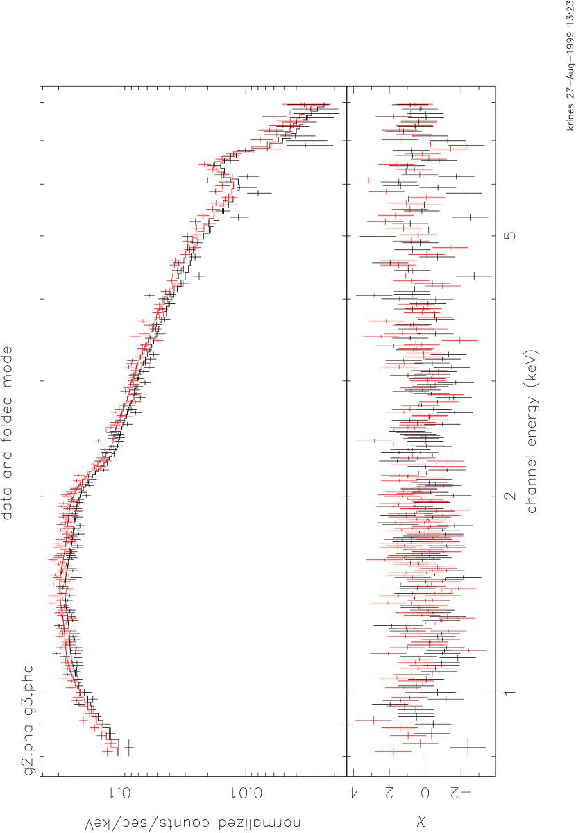
Figure 10: ASCA GIS spectrum of A576. The solid line is the best-fit single-temperature Raymond-Smith thermal plasma model.

We obtain acceptable fits by assuming that the gas is isothermal. More complicated models are thus unnecessary. Our best-fit model has an ICM temperature of 3.77$\pm 0.10$ keV with an iron abundance 0.27$\pm 0.05$ cosmic. Uncertainties are 68% confidence limits for one parameter. Figure 10 shows the X-ray spectrum and the best-fit model. This temperature is 1.7$\sigma$ less than the temperature of 4.3$\pm 0.3$ keV (David et al. 1993) from Einstein MPC data and 2.5$\sigma$ less than $4.02\pm 0.07$ keV from an independent analysis of the ASCA data (White (2000)).

We calculate the expected flux between 0.01 and 100.0 keV from the best-fit model, yielding an essentially bolometric flux of $4.30\times 10^{-11}$ ergs cm^-2 s^-1. We calculate a bolometric luminosity of $0.71\times 10^{44}h^{-2}$ ergs s^-1 (we assume $q_{0}$ = 0.0) in agreement with $0.73\times 10^{44}h^{-2}$ ergs s^-1 from Einstein MPC data (David et al. (1993)). The 0.3-3.5 keV luminosity is $0.46\times 10^{44}h^{-2}$ergs s^-1, in excellent agreement with M96, who find a luminosity of $0.45\times 10^{44}h^{-2}$ergs s^-1 from the Einstein IPC data assuming an ICM temperature of 4.3 keV.

M96 found that a two-temperature Raymond-Smith model improved the fits to the Einstein spectrum. We test this result by adding a second thermal component to our isothermal model, but the fitting routine forces the temperature of the second component to be extremely small ($\lesssim 0.1$keV), suggesting that no second component is needed to explain the more complete ASCA data. This result contradicts the lower central temperature found with Einstein SSS data (Rothenflug et al. (1984)). An independent anaysis of the ASCA data (White (2000)) suggests that A576 has a flat temperature profile and no cooling flow.

We use Einstein IPC data to analyze the surface brightness profile. Previous studies (Jones & Forman (1984); 1999; M96) fit the profile to the hydrostatic-isothermal $\beta_{x}$ model (Cavaliere & Fusco-Femiano (1976)) and found $\beta_{x}=0.45-0.53$, and 0.58-0.72 and core radius $a=50-70,$ and $90-160~{}h^{-1}{\rm kpc}$ for Jones & Forman (1999) and M96 respectively. These models yield central gas and electron number densities of $\rho_{0}=3.6(2.3)\times 10^{-27}$ g cm^-3 and $1.9(1.2)\times 10^{-3}$cm^-3 respectively. M96 suggest that the disagreement arises from fitting different radial ranges; Jones & Forman extend their analysis to larger radius than M96. We consider both models below.

4.1 X-ray Mass Profile

With the assumptions of hydrostatic equilibrium, negligible non-thermal pressure, and spherical symmetry, the gravitational mass inside a radius r is

$$M_{tot}(<r)=-\frac{kT}{\mu m_{p}G}\Bigl{(}{{d\ln\rho_{gas}}\over{d\ln r}}+{{d\ln T}\over{d\ln r}}\Bigr{)}r$$ (6)

(Fabricant, Lecar, & Gorenstein (1980)). For a uniform temperature distribution, the second term on the right hand side vanishes. We then only need to determine the gas temperature and the density distribution of the gas to calculate the gravitational mass. Under the standard hydrostatic-isothermal $\beta_{x}$ model, the mass is related to $\beta_{x}$ and $a$ by

$$M_{tot}(<r)=\frac{3kT\beta_{x}r^{3}}{\mu m_{p}Ga^{2}(1+(\text@frac{r}{a})^{2})}\newline =5.65\times 10^{13}\beta_{x}T_{\mbox{keV}}\frac{r^{3}}{a^{2}+r^{2}}h^{-1}M_{\odot}$$ (7)

where $M_{tot}(<r)$ is the total gravitational mass within a radius $r$ and the numerical approximation is valid for $T_{\mbox{keV}}$ in keV and $r$ and $a$ in $h^{-1}{\rm Mpc}$.

We use Equation 6 to calculate the total mass profile of A576 within 1.5$h^{-1}{\rm Mpc}$; the estimate outside $\sim 0.5~{}h^{-1}{\rm Mpc}$ is an extrapolation. We use our ASCA-derived temperature with the results of both M96 and Jones & Forman (1999) to estimate the mass profile. Figure 11 shows these profiles as well as the gas mass profile for the M96 parameters. We also display an estimate of the cluster mass based on spherical deprojection (White, Jones & Forman 1997). This estimate is $M\approx 1.07\times 10^{14}~{}h^{-1}M_{\odot}$ at $r=0.299~{}h^{-1}{\rm Mpc}$ and is larger than either $\beta_{x}$ model estimate.

Evrard et al. (1996) develop a method to reduce the scatter in cluster mass estimates by relying solely on the emission-weighted gas temperature $T_{X}$ within a radius where the mean density is 500 times the critical density. This radius, denoted by $r_{500}$, varies with $T_{X}$ as

$$r_{500}=(1.24\pm 0.09)\Bigl{(}\frac{T_{X}}{10\mbox{keV}}\Bigr{)}^{1/2}h^{-1}\mbox{Mpc}.$$ (8)

The mass within $r_{500}$ is approximately

$$M_{500}(T_{X})=1.11\times 10^{15}\Bigl{(}\frac{T_{X}}{10\mbox{keV}}\Bigr{)}^{3/2}~{}h^{-1}M_{\odot}$$ (9)

and has an average estimated-to-true mass ratio of 1.00 with a standard deviation of 8-15%. For A576, this procedure yields $M_{500}=2.57\times 10^{14}~{}h^{-1}M_{\odot}$ at $r_{500}=0.76\pm 0.16~{}h^{-1}{\rm Mpc}$. This semi-empirical estimate of $r_{500}$ agrees with our more direct estimate of $r_{500}=0.96\pm 0.05~{}h^{-1}{\rm Mpc}$ from the caustics. From the infall mass profile, we estimate $M_{500}=(5.1\pm 0.5)\times 10^{14}~{}h^{-1}M_{\odot}$.

Within $\sim 0.5~{}h^{-1}{\rm Mpc}$, the infall mass profile is a factor of $\sim$2.5 larger than the isothermal X-ray mass profiles and a factor of $\sim$1.8 larger than the deprojection estimate of White et al. (1997). M96 find a similar difference between X-ray mass estimates and other kinematic mass estimates of A576. These differences could be due to non-thermal pressure support, nonisothermality, or asymmetry.

4.2 Gas Mass Fraction

Using only X-ray data, the gas mass fraction $f_{g}$ (the fraction of total gravitational mass in hot gas) increases with radius (Figure 12), suggesting that the hot gas is more extended than the mass distribution, in agreement with previous studies (David, Jones, & Forman (1995); Markevitch & Vikhlinin (1997); Ettori & Fabian (1999)). The gas mass fraction is $\sim 0.07h^{-3/2}$ at $R_{p}=0.5~{}h^{-1}{\rm Mpc}$, less than (but consistent with) the average value of gas mass fractions in the most luminous clusters (e.g., White et al. (1993); Evrard (1997); Mohr, Mathiesen, & Evrard (1999); Ettori & Fabian (1999)). In hydrodynamical simulations (e.g. Evrard (1997) and references therein), the hot gas is more extended than the dark matter because of the shock heating originating during the merging of the halos which will form the cluster. In real systems, energy ejection from supernovae could also contribute to heat the gas.

We observe a similar trend of increasing gas mass fraction with radius when we use the best-fit NFW infall mass profile to calculate the gas mass fraction (Figure 12). Because the infall mass profile exceeds the X-ray mass profile, the inferred gas mass fraction ($\sim 0.03h^{-3/2}$ at $R_{p}=0.5~{}h^{-1}{\rm Mpc}$) is smaller.

5 Estimating the Contribution of Background Galaxies

Within the completeness limit of our redshift survey, the elimination of background galaxies is straightforward; we simply remove non-member galaxies using the caustics in the projected radius-redshift diagram. We must estimate the background statistically at magnitudes fainter than $m_{R}=16.5$. For $16.5<m_{R}<18.0$, we only have spectroscopy in the central region ($<0.^{\circ}75$ radius; Mohr et al. (2000)). In this central region, the survey is 91, 79, and 60% complete to limiting magnitudes of $m_{R}=17.0$, 17.5, and 18.0 respectively. We assume that this region is sufficiently large to represent a fair sample of the background over the entire field. We then calculate the number of background galaxies in each 0.5 mag bin by assuming that the fraction of cluster members is the same for galaxies with and without redshifts.

It is important to determine whether the survey of A576 contains any background or foreground groups or clusters of galaxies; these groups would lead to a localized enhancement in the number density of galaxies. Applying the adaptive kernel method (Pisani (1993)) to all redshifts in our sample yields the estimated parent distribution shown in Figure 13. A576 is very prominent. This distribution shows a background concentration of galaxies at $19,700~{}{\rm km~{}s}^{-1}$; these galaxies concentrate in a region $\sim 0.^{\circ}50-0.^{\circ}75$ from the center of A576 (Figure 14). This concentration suggests an enhancement of background light in this region relative to a randomly selected field. Because we use this region to estimate the background, we may overestimate the background luminosity density across the entire region. However, the excess background may be present across the entire field.

To estimate the variation of galaxy backgrounds in randomly selected fields, we analyze four $1^{\circ}\times 1^{\circ}$ images of fields in the Century Survey (Brown et al. (2000)) taken on the same nights with the same observing setup as the A576 data. Due to large-scale structure, the background counts vary more than expected from a Poisson distribution; the mean number of galaxies in a field is 121 and the variance is 19.2 (the four fields contain 149, 118, 110, and 107 galaxies). Weighted by luminosity, the variance is 21%. Figure 15 shows the magnitude distributions from these fields. For comparison, we show the estimate from the central region of A576. In the magnitude range of interest ($16.5<m_{R}<18.0$), the estimate of background light from the average of the Century Survey fields is $\sim 40\%$ (roughly 2 $\sigma$) smaller than that from the central region of A576. Because this enhanced background may or may not be present across the entire region, we estimate that the background subtraction is accurate to $\sim 40\%$ on scales $\gtrsim 1^{\circ}$ square.

A third method of estimating the background is to assume that the surface number density of cluster galaxies becomes negligible at the outermost radii of our survey; we require that the cluster number density be no less than that of known cluster galaxies. We attribute additional surface number density to background galaxies. By measuring this number density as a function of limiting magnitude, we can estimate the number counts of background galaxies and the total background light. Figure 15 shows the magnitude-number distribution from this method. Because this method assumes that no faint galaxies at large radii are infall members, this method should overestimate the background light. The ratio of the background light estimates calculated from the central region, the number density profile, and Century Survey fields are 1.14 : 1 : 0.67.

The background estimates from the central region of A576 and from its outskirts agree surprisingly well. Thus, our determination of the background light seems to be a reasonable estimate of the background luminosity density across the entire region studied. We adopt the background values from the number density profile, which are intermediate between the values for the central region and the Century Survey.

This estimate of the background is likely an overestimate. It is conservative in the sense that it tends to underestimate the cluster light. Because the amount of background light enclosed increases with radius, the effects of overestimating the background also increase with radius.

6 Surface Number Density Profile

One approach to studying the relative distributions of mass and light in a cluster is to compare the infall mass profile with the galaxy surface number density profile. We calculate the surface number density profiles with two different galaxy samples $m_{16.5}$ and $m_{18}$ where the subscript denotes the magnitude limit of the sample. For both samples, we exclude non-members with $m_{R}<$16.5. The $m_{16.5}$ sample provides a lower limit on the asymptotic number density for fainter limits. We subtract a constant surface number density from the $m_{18}$ sample using the method described in $\S 5$.

If light traces mass, the surface number density profile should closely resemble the infall mass profile ($\S 3$). The projection of the NFW profile yields a surface density profile $\Sigma(R_{p})$

$$\Sigma_{NFW}(\tilde{R})=\frac{N_{c}}{\pi{\rm ln}(4/e)a_{NFW}^{2}(\tilde{R}^{2}-1)}[1-X(\tilde{R})]$$ (10)

where $\tilde{R}=R/a_{NFW}$ is the projected radius in units of the core radius, $N_{c}$ is the number of galaxies within $a_{NFW}$, and

$$X(\tilde{R})=\frac{{\rm sec}^{-1}{\tilde{R}}}{\sqrt{\tilde{R}^{2}-1}}$$ (11)

Similarly, the projection of the Hernquist profile can be written as

$$\Sigma_{Hern}(\tilde{R})=\frac{2N_{c}}{\pi a_{Hern}^{2}(\tilde{R}^{2}-1)^{2}}[(2+\tilde{R}^{2})X(\tilde{R})-3]$$ (12)

(Mahdavi et al. (1999)).

Table 4 gives the results of our fits. For the NFW profile, the scale radius of the surface number density profile for the $m_{16.5}$ sample agrees with that for the mass profile. The scale radii for the $m_{18}$ sample and for the Hernquist fit to the $m_{16.5}$ sample are larger than the best-fit scale radii for the respective mass profiles. We display the surface number density profiles and the best-fit models in Figure 16. There appears to be a relative excess of galaxies in the magnitude range $16.5<m_{R}<18.0$ between 1 and 2$h^{-1}{\rm Mpc}$. This excess leads to significantly larger scale radii for the $m_{18}$ sample than for the $m_{16.5}$ sample. This discrepancy may suggest the presence of a background cluster of galaxies ($\S 5$). The surface number density profile yields some evidence that galaxies are more extended than the dark matter, just as hot gas in the core is more extended than the dark matter. This evidence is stronger for the Hernquist model than for the NFW model; note that the Hernquist models produce better fits. One possible explanation of this difference is luminosity segregation, which we investigate next.

7 Luminosity Segregation

To convert to absolute magnitudes, we assume that all galaxies are at the distance of the cluster center; thus, $M_{R}=m_{R}-35.29-A_{R}+5~{}{\rm log}~{}h$, where we estimate the dust extinction coefficient $A_{R}$ from the dust maps of Schlegel, Finkbeiner, & Davis (1998) as listed in Table 1. We obtain the color excess at each galaxy position; the inferred extinction values range from 0.13 to 0.26 across the field.

Figure 17 shows the luminosity distribution for all galaxies with $m_{R}<18$ after removing all non-cluster galaxies with $m_{R}<$16.5, the completeness limit of our spectroscopic sample. The contribution of background galaxies steepens the distributions at $M_{R}\gtrsim-19$. In the outer regions, the number counts begin to resemble $N(m)\propto m^{0.6}$.

Luminosity segregation, if present, should be most apparent for the most luminous galaxies. In a large sample of clusters, Adami et al. (1998a) claim luminosity segregation among (on average) the four brightest members of each cluster. As a simple test of luminosity segregation, Figure 18 shows absolute magnitude versus radius for cluster galaxies in the complete $m_{16.5}$ sample. Significant segregation requires increasing absolute magnitude with radius. In fact, the three brightest galaxies in A576 are all $>1~{}h^{-1}{\rm Mpc}$ from the center, and the brightest cluster galaxy is $3.5~{}h^{-1}{\rm Mpc}$ from the center, more than two Abell radii away. The most luminous galaxy appears to be a normal S0 galaxy, with an absorption dominated spectrum and no close companions. The next two most luminous galaxies also have absorption dominated spectra, but one of them has a close companion.

As a quantitative test of luminosity segregation, we compare the cumulative luminosity distributions for all cluster galaxies with $M_{R}<-19.0$ (our spectroscopic completeness limit) inside and outside a radial cutoff (e.g., Figure 19). We vary this cutoff radius from $0.05-2.50~{}h^{-1}{\rm Mpc}$ in steps of $0.05~{}h^{-1}{\rm Mpc}$ and perform a K-S test for each division. The only radial division that yields a separation at greater than a 90% confidence level is at $1.45~{}h^{-1}{\rm Mpc}$ (95.2% confidence). However, the difference between the samples suggests luminosity anti-segregation, i.e., the outer sample is marginally brighter than the inner sample.

To test the sensitivity of this result to the magnitude limit, we repeat the analysis using a magnitude cutoff of $M_{R}<-20.7$, approximately the value of $M_{*}$ for the entire region ($\S 8.1$). With this cutoff, there is no significant difference at any radius (see Figure 19). Combined with the result that the three most luminous galaxies in the sample are located far outside the core, we conclude that there is no significant evidence of luminosity segregation in A576.

8 Luminosity Function and Light Profile

8.1 Luminosity Function

By correcting the luminosity function for the background counts ($\S 5$), we obtain the luminosity function shown in Figure 17. Because we explicitly assume that few faint member galaxies are present at large radii, we are unable to constrain the faint-end slope of the luminosity function.

We calculate the best-fit Schechter (1976) luminosity function,

$$\frac{dn}{dM}\Bigg{|}_{M}\propto 10^{0.4(1+\alpha)(M_{*}-M)}{\rm exp}[-10^{0.4(M_{*}-M)}]$$ (13)

in the range $-22.5<M_{R}<-19$, where $M_{*}$ is the characteristic absolute magnitude and $\alpha$ is the slope at the faint end. We find the best-fit form by minimizing $\chi^{2}$. The parameters for the total luminosity function, $M_{*}=-20.7\pm 0.4$ and $\alpha=-1.0\pm 0.3$ (95% confidence limits), are consistent with those of M96, LCRS (Lin et al. (1996), a hybrid Gunn $r$-Kron-Cousins $R$ system), and the Century Survey (Geller et al. (1997), an R-selected survey). The fit yields $\chi^{2}=3.5$ for 10 degrees of freedom; a single Schecter function is therefore a good model of the data.

8.2 Light Profile

We calculate the light profiles for the $m_{16.5}$ and $m_{18}$ using the estimated background light from the asymptotic number counts around A576 (Figure 20). Using the absolute R-band magnitude of the Sun ($M_{R}=4.3$ ; Zombeck 1990), we calculate the total light profiles for these subsamples. The potential overestimate of the background leads to an underestimate of the light profile, particularly at large radii. The $m_{18}$ sample yields an upper limit to the light profile by assuming that all galaxies without redshifts are cluster members (a lower limit comes from the $m_{R}<16.5$ sample).

Because the line-of-sight distribution of the galaxies is unknown, the observed light profile is the projection of the actual light profile. We therefore compare the observed light profile to the analytic forms in $\S 5$, replacing $N_{c}$ with $L_{c}$, the amount of light enclosed within the scale radius $a$. The cumulative projected light profile for the Hernquist model has the simple form

$$L(<R_{p})=L_{tot}a^{2}\frac{X(\tilde{R})-1}{1-\tilde{R}^{2}}$$ (14)

where $L_{tot}$ is the total luminosity of the system (Hernquist (1990)). The results, shown in Table 5, reveal that the scale radii of the best-fit NFW profiles agree with that of the infall mass profile, whereas the Hernquist light profiles have scale radii a factor of $\sim 1.8-3$ larger than the best-fit mass profile. Figure 21 displays the best-fit profiles of each type. The values of $\chi^{2}$ are rather large in all cases. It is evident from inspection of Figure 21 that the observed light profile does not fall off as steeply as the NFW or Hernquist profiles at large radii ($R_{p}\gtrsim 2h^{-1}{\rm Mpc}$). If we convert the projected mass profile into a projected light profile by assuming a constant mass-to-light ratio (Figure 20), the predicted light profile increases more slowly than the observed light profile. This result suggests that the difference in scales between the mass and light profiles can not be explained by projection effects unless there are significant departures from spherical symmetry (e.g., our line of sight is perpendicular to the disk of an oblate system).

9 Mass-to-Light Profile

With the independently derived mass and light profiles, we can now calculate the R-band mass-to-light profile of A576 out to $\sim 4~{}h^{-1}{\rm Mpc}$, the limit of the infall mass profile. By dividing the mass profile by the projected light profile, we obtain the mass-to-light profile shown in Figure 22. $M/L_{R}(<R_{p})$ is largest in the core ($\sim 700~{}h$) and decreases smoothly to the limiting radius of $\sim~{}4~{}h^{-1}$ Mpc, where $M/L_{R}\sim 300h$. We use the lower limits on the light profile to calculate “upper limits” on $M/L_{R}(<R_{p})$. These upper limits do not include the uncertainties in the mass profile; they demonstrate that the decreasing mass-to-light profile is not a result of underestimating the background light (in $\S 5$, we explain why we may overestimate the background light). We fit the profiles from the $(m_{18})$ sample to a straight line ($M/L_{R}=aR_{p}+b$) and to a constant value ($M/L_{R}=b$) using weighted least squares. Table 6 displays the results of these fits. The best-fit straight lines have negative slopes with high significance. Because the true $M/L$ is always positive, the actual $M/L$ profile extrapolated to arbitrarily large radius cannot be a straight line with a negative slope. Again, because the values of $M(<R)$ are not independent, the values of $\chi^{2}$ are only indicative. However, this exercise shows that a decreasing profile yields a much better fit than a flat one.

We note again that the light profile is the two-dimensional projection of the three-dimensional light profile; the deprojected mass-to-light profile of a spherically symmetric system would decrease more steeply than the ones presented here (see also Figure 20). As an example, we take the best-fit Hernquist mass profile, project it according to Equation 14 (assuming spherical symmetry), and divide it by the projected light profile. The resulting projected-mass to projected-light profile, shown in Figure 22, is larger in the inner $\sim 1h^{-1}{\rm Mpc}$ than the radial-mass to projected-light profile.

This mass-to-light profile is an integrated profile, i.e., $M/L_{R}(<R_{p})=~{}M(<R_{p})/L(<R_{p})$. The significance of the decreasing profile is more dramatic as a differential profile where $M/L_{R}(R_{p})=\delta M(R_{p})/\delta L(R_{p})$ (Figure 23). Again, a decreasing mass-to-light profile yields a better fit than a flat one (Table 6). The outermost value of this profile ($\sim 100~{}h$) should be closest to an estimate of the universal value of $M/L_{R}$. Interestingly, this value agrees with the mass-to-light ratios of some elliptical galaxies (Mushotzky et al. (1994); Bahcall, Lubin, & Dorman (1995)).

10 Discussion

A decreasing mass-to-light profile is perhaps surprising. One immediately wonders what systematic effects could mimic a decreasing $M/L_{R}$ profile. Is the mass profile incorrect? The infall mass profile yields larger values than X-ray estimates in the inner regions and lower values than virial theorem estimates in the outer region. Non-thermal pressure support, nonisothermality, and deviations from virial equilibrium are plausible explanations for these effects. Another unknown systematic effect is the actual distribution of galaxy orbits. However, simulations suggest that this effect is not large (D99). The infall mass profile itself is uncertain by a factor of 2. Hidden systematic effects could affect the shape of the mass profile, a possibility we plan to explore with other systems. The infall mass profile is unstable from $1.5-2.2h^{-1}$ Mpc, but beyond this range, $M/L_{R}$ continues to decrease even though the mass profile is well determined. A Jeans analysis of the virial region will provide an interesting check on the infall mass profile (Mohr et al. (2000)); preliminary results suggest good agreement between the infall mass profile and the Jeans mass profile. We note also that the X-ray mass found by White et al. (1997) provides a lower mass limit at small radius. While this mass estimate is smaller than the infall mass estimate, it is not sufficient to reconcile the observations with a constant mass-to-light ratio.

Is the light profile poorly estimated? In the inner regions, we use SExtractor magnitudes, which may underestimate the diffuse light associated with Brightest Cluster Galaxies (BCGs) by $\sim 50\%$ (Gonzalez et al. (2000)). Even though A576 has no cD galaxy, diffuse light near the center of the cluster may partially account for the observed decreasing M/L profile. The magnitude of this effect ($\sim 20\%$ of the total light within $1.5~{}h^{-1}{\rm Mpc}$), however, is not sufficient to reconcile the observed $M/L_{R}$ profile with a constant value. Background subtraction always contains some uncertainty; we show the limits of this uncertainty based on galaxies reliably contained within the infall region. The background light we assume exceeds that in randomly selected fields, and two independent estimates of the background agree remarkably well. The shape of the $M/L_{R}$ profile is insensitive to the magnitude limit. The surface number density profile also supports a larger scale for the galaxies than for the mass. We note that any systematic underestimate of total galaxy light (e.g., missing halo light) would likely affect the magnitudes of all galaxies. Such an effect would change the absolute value of $M/L_{R}$ but would be unlikely to alter the shape of the profile.

Are projection effects skewing our results? According to the infall model, the mass profile is a true radial profile; the light profile is the two-dimensional projection of the actual light profile. Assuming that luminosity density decreases monotonically with radius, the projected light profile is steeper than the actual light profile. This effect would increase the significance of the decreasing mass-to-light profiles presented here. Departures from spherical symmetry could also affect the mass-to-light profile; looking down the barrel of a prolate spheroid would exaggerate the decrease in M/L; looking at the disc of an oblate spheroid would mitigate it. There are no obvious indications of oblate or prolate structure in the sky distribution of infall members (Figure 6). Analysis of other systems should provide an important check on these projection effects.

Is the decreasing mass-to-light profile an effect of calculating the luminosity from R-band photometry? Galaxies in the cores of clusters are redder than those far outside the cores. This effect causes the R-band light density profile to decrease more steeply with radius than a B-band light density profile. This effect would oppose the apparent trend of a radially decreasing mass-to-light profile.

M96 demonstrate that the emission-dominated galaxies have different kinematic properties than absorption-dominated galaxies. On this basis, M96 removes the light contribution from emission-dominated galaxies in calculating the mass-to-light ratio. Because many of these emission-dominated galaxies are in the infall region but probably not inside the virial radius, the mass-to-light profile is biased low in the central regions and high in the outer regions.

Finally, we note a curious feature of the D99 simulations. For $\Lambda CDM$ models, the mass-to-light profiles (in B band relative to the global value) show a decreasing trend similar to that shown here. Clusters in a $\tau CDM$ model produce the opposite effect, mass-to-light profiles which increase with radius. D99 attributes this effect to the deficit of blue galaxies in the centers of clusters in the $\Lambda CDM$ model, but later analysis reveals a similar effect for mass-to-light profiles measured in I band. This result suggests that the decreasing mass-to-light profile may contain information on the underlying cosmology.

11 Conclusions

We calculate the mass profile of Abell 576 to $\sim 4~{}h^{-1}{\rm Mpc}$ from the observed infall pattern in redshift space. The amplitude of the resulting mass profile is larger than determined from X-ray observations to their limiting radius of 0.5 $h^{-1}$ Mpc and smaller than virial mass estimates at larger radius. The infall mass profile agrees extremely well with an NFW profile or a Hernquist (1990) profile, and it is strongly inconsistent with an isothermal sphere profile. This result agrees well with a similar analysis of Coma by GDK. Our best-fit mass profile implies that the fraction of gravitational mass contained in hot gas increases with radius to the limit of the X-ray data, in agreement with previous studies of other clusters (e.g., David, Jones, & Forman (1995); Markevitch & Vikhlinin (1997); Ettori & Fabian (1999)) and simulations (White et al. (1993); Evrard (1997)). The hot gas therefore appears to be more extended than the dark matter.

The decreasing amplitude of the caustics suggests that the mass increases more slowly than for an isothermal sphere. This inference is supported by fitting mass profiles to the data. GDK found that the NFW profile describes the mass profile of Coma much more accurately than an isothermal sphere profile, and Figure 1 of CYE clearly shows the existence of radially decreasing caustics in the composite CNOC cluster. Many clusters therefore show evidence of mass profiles shallower than an isothermal sphere; the masses of clusters probably increase no faster than ${\rm ln}(R_{p})$ at large radius.

Using photometric data from a large area surrounding the cluster, we find little evidence for luminosity segregation. In fact, there is some evidence of luminosity antisegregation; the three brightest cluster galaxies lie far outside the center of the cluster.

The R-band mass-to-light ratio is largest in the core ($\sim 700~{}h$) and decreases smoothly to the limiting radius $\sim~{}4~{}h^{-1}$ Mpc, where $M/L_{R}(<R_{p})\sim 300h$. The decrease is more dramatic in the differential mass-to-light profile. At the limit of our sample, $dM/dL\sim 50-150h$. The luminosity density from the Century Survey is $\rho_{L}=\phi^{*}L^{*}\Gamma(2+\alpha)=6.0\pm 2.6\times 10^{8}h^{3}~{}$Mpc^-3 which yields $(M/L)_{crit}=459\pm 199h$ (Geller et al. (1997)). Our estimate of the global value of $M/L$ thus implies $\Omega_{m}\lesssim 0.22\pm 0.1$, or $\Omega_{m}\lesssim 0.4$ at a 95% confidence level. This estimate of $\Omega_{m}$ is an upper limit due to the unknown contribution of faint ($m_{R}>18$) galaxies. Note that using the luminosity function parameters from the LCRS (Lin et al. (1996)) yields a significantly smaller luminosity density corresponding to $(M/L)_{crit}=1000\pm 150h$. Adopting this luminosity density reduces our estimate of the matter density to $\Omega_{m}\lesssim 0.10\pm 0.05$. The decreasing $M/L$ profile suggests that the dark matter is more concentrated than the optical light of the galaxies. We consider possible systematic effects ($\S 10$) and find that they generally oppose the decreasing mass-to-light ratio. If general, our results place strong constraints on possible variations of mass-to-light ratios with scale as well as on the global value of $\Omega_{m}$.

Photometric observations in other bandpasses would allow an examination of the effects of stellar populations on the mass-to-light profile. Similar studies of other clusters, particularly studies of clusters with better defined infall regions at large radius, should test the generality of our results.

Figure 1: Comparison of magnitudes from the two nights for galaxies in the central region. For $m_{R}<18$, the zero-point offset is -0.002 mag with $\sigma\approx 0.09$ mag. The scatter increases with apparent magnitude.

Figure 3: Fraction of galaxies with measured redshifts as a function of $m_{R}$ magnitude. The solid line shows galaxies with $R_{p}<1^{\circ}$, the dashed line shows galaxies at larger radii. We also display the total number of galaxies in each bin (thick lines).

Figure 4: Redshifts as a function of projected radius in A576. The solid lines are the caustics determined from our adaptive kernel estimate with 1-$\sigma$ error bars.

Figure 5: Dependence of caustic location on the parameter $q$, the ratio of velocity uncertainty to positional uncertainty. From top to bottom, the caustics are fit with $q=10$, 25, and 50.

Figure 6: Distribution of cluster and field galaxies on the sky. Open circles, filled circles, and crosses represent cluster members, members with $m_{R}<16.5$, and background galaxies respectively.

Figure 7: Mass profile of A576. The filled squares are from the adaptive kernel estimate of the caustics with $1-\sigma$ uncertainties shown. The upper and lower filled hexagons are virial mass estimates (Girardi et al. 1998) omitting and including the surface term respectively; the filled hexagon at small radius is an interpolation by Girardi et al. discussed in the text. Crosses show our virial and projected mass estimates, the star shows an X-ray mass estimate ($\S 4.1$, White, Jones & Forman (1997)). The solid, dashed, and dash-dot lines are the best-fit NFW, Hernquist, and isothermal sphere profiles respectively.

Figure 8: Mass density profile of A576. Lines have the same definitions as in Figure 7.

Figure 9: Velocity dispersion profile for A576. Open squares show the velocity dispersion profile $\sigma_{p}(R_{p})$. Filled squares show the cumulative velocity dispersion profile $\sigma_{p}(<R_{p})$. Dashed and dash-dotted lines indicate the predicted profiles for the best-fit Hernquist and NFW profiles respectively assuming isotropic orbits ($\beta=0$).

Figure 11: Mass profile of A576 derived from X-ray observations under the assumption of the hydrostatic-isothermal $\beta_{x}$ model and parameters from Jones & Forman (1999, dash-dotted line) and M96 (dashed line). The solid line is the gas mass profile and the vertical line at $R_{P}=0.5~{}h^{-1}{\rm Mpc}$ shows the limit of the X-ray data. Filled squares show the infall mass profile. The open hexagon and star are X-ray mass estimates from White et al. (1997) and from the estimator of Evrard et al. (1996) respectively.

Figure 12: Gas mass fraction profile. $M_{gas}$ is taken from the X-ray temperature and density profile, $M_{tot}$ is the best-fit X-ray mass profile (dashed line) or Hernquist (solid) or NFW (dash-dot) infall mass profile. The vertical line is the limit of the X-ray data.

Figure 13: Adaptive kernel estimate of $f_{ka}(cz)$, the velocity distribution function. Arrows indicate the peak and limits of A576 and the limits of a background concentration of galaxies.

Figure 14: Distribution on the sky of background concentration of galaxies. The cross marks the X-ray center of A576.

Figure 15: Apparent magnitude distribution of four randomly selected fields from the Century Survey (solid lines). The dashed line is the background estimated from the central region of A576; the dash-dot line is estimated from the asymptotic number density profile.

Figure 16: Surface number density profile for A576. Squares show the profile calculated from $m_{R}<16.5$, hexagons show the background-subtracted profile for $m_{R}<18$. The solid and dashed lines are the best fit NFW and Hernquist profiles respectively for the $m_{R}<16.5$ sample.

Figure 17: Luminosity function for entire region. Filled and open squares are calculated with and without background subtraction respectively. The vertical line is the limit of our survey. The curve indicates the best-fit Schechter luminosity function for $M_{R}<-19$.

Figure 18: Absolute magnitude versus projected radius. Significant luminosity segregation requires that absolute magnitudes increase with radius. The three most luminous galaxies all have $R_{p}>1~{}h^{-1}{\rm Mpc}$.

Figure 19: (a) Cumulative absolute magnitude distributions of galaxies inside (solid lines) and outside (dashed lines) $R_{div}=1.45~{}h^{-1}{\rm Mpc}$. The outer sample is brighter than the inner with 95% confidence for $M_{R}<-19.0$. (b) Same for $R_{div}=1.45~{}h^{-1}{\rm Mpc}$ and $M_{R}<-20.7$.

Figure 20: R-band luminosity profile of A576 (crosses). We exclude all non-cluster galaxies with $m_{R}<16.5$. The faint solid and dash-dot lines are the profiles calculated from $m_{R}<18$ galaxies with and without background subtraction respectively. The heavy solid and dashed lines are the best-fit Hernquist light and mass profiles (converted with an arbitrary mass-to-light ratio).

Figure 21: R-band luminosity density profile of A576. Symbols are as in Figure 16. The solid and dashed lines are the best fit NFW and Hernquist profiles respectively for the $m_{R}<16.5$ sample.

Figure 22: Cumulative mass-to-light profile of A576 calculated from the infall mass profile and the projected light profile. Squares estimate the light profile from galaxies with $m_{R}<18$; upper limits include only light from confirmed members ($m_{R}<16.5$). The dash-dotted line indicates the projected best-fit Hernquist mass profile divided by the projected light profile.

Figure 23: Differential mass-to-light profile. Squares represent the $m_{18}$ luminosity profile. Upper limits reflect the minimum light associated with the cluster.

Table 1: Photometric and Spectroscopic Data

RA	DEC	$cz$	$\sigma_{cz}$	$m_{R}$	$\sigma_{m_{R}}$	$A_{R}$
(J2000)	(J2000)	(${\rm km~{}s}^{-1}$)	(${\rm km~{}s}^{-1}$)
7 10 58.32	+56 29 25.4	39154	37	15.84	0.06	0.15
7 10 59.40	+56 30 15.8	14569	17	16.11	0.06	0.15
7 11 03.94	+56 39 38.2	16042	15	16.38	0.06	0.13
7 11 04.13	+56 39 46.4	15918	16	15.92	0.06	0.13
7 11 09.26	+56 02 13.2	13780	29	15.59	0.06	0.16

Table 2: Spectroscopic Data

RA	DEC	$cz$	$\sigma_{cz}$
(J2000)	(J2000)	(${\rm km~{}s}^{-1}$)	(${\rm km~{}s}^{-1}$)
6 53 01.56	+56 15 35.3	10057	32
6 54 33.82	+55 14 41.6	14215	39
6 55 15.14	+55 28 42.6	16899	29
6 55 48.17	+56 04 56.3	19347	43
6 56 00.38	+55 24 02.2	7908	26

Table 3: Mass Profile Fit Parameters

Profile	$a$	95%	$C$	95%	$\chi^{2}$	$\nu$
	$h^{-1}{\rm Mpc}$	$h^{-1}{\rm Mpc}$	$10^{15}M_{\odot}/{\rm Mpc}$	$10^{15}M_{\odot}/{\rm Mpc}$
NFW	0.13	0.11-0.16	2.9	2.7-3.2	7.23	25
Hernquist	0.43	0.37-0.49	2.5	2.3-2.7	1.64	25
Isothermal	–	–	0.322	0.308-0.334	179	26

Table 4: Surface Number Density Profile

Profile	Sample	$N_{c}$	$a$	95%	$\chi^{2}$	$\nu$	Prob
NFW	$m_{16.5}$	124	0.12	0.08-0.18	33.7	20	0.03
NFW	$m_{18}$	340	0.42	0.24-0.74	10.4	20	0.96
Hernquist	$m_{16.5}$	605	0.68	0.58-0.82	28.9	20	0.09
Hernquist	$m_{18}$	1060	1.20	0.80-1.64	11.5	20	0.93

Table 5: Projected Light Profile

Profile	Sample	$a$	95%	$L_{c}$	95%	$\chi^{2}$	$\nu$
		$h^{-1}{\rm Mpc}$	$h^{-1}{\rm Mpc}$	$10^{10}L_{\odot}$	$10^{10}L_{\odot}$
NFW	$m_{16.5}$	0.15	0.12-0.18	59	56-62	333	22
NFW	$m_{18}$	0.45	0.34-0.59	152	124-188	17.9	22
Hernquist	$m_{16.5}$	0.76	0.70-0.84	260	252-272	347	22
Hernquist	$m_{18}$	1.27	1.03-1.59	470	400-560	26.8	22
CumHern	$m_{16.5}$	0.86	0.85-0.87	245	243-248	2524	365
CumHern	$m_{18}$	1.47	1.45-1.48	459	456-463	6121	1846

Table 6: Fits of M/L Profile to $M/L_{R}=aR_{p}+b$

Type	Sample	a	b	$\chi^{2}$	$\nu$
Int	$m_{16.5}$	-62$\pm 4$	651$\pm 10$	2.0	22
Int	$m_{18}$	-90$\pm 5$	592$\pm 13$	5.5	22
Int	$m_{16.5}$	–	516$\pm 14$	25	23
Int	$m_{18}$	–	378$\pm 10$	81	23
Diff	$m_{16.5}$	-158$\pm 31$	583$\pm 67$	127	22
Diff	$m_{18}$	-109$\pm 27$	376$\pm 61$	206	22
Diff	$m_{16.5}$	–	263$\pm 10$	278	23
Diff	$m_{18}$	–	145$\pm 6$	354	23

References

- Abell (1958) Abell, G.O. 1958, ApJS, 3, 211
- Aceves & Perea (1999) Aceves, H. & Perea, J. 1999, A&A, 345, 439
- (3) Adami, C., Biviano, A., & Mazure, A. 1998, A&A, 331, 439
- (4) Adami, C., Mazure, A., Katgert, P. & Biviano, A. 1998, A&A, 336, 63
- Anupama et al. (1994) Anupama, G.C., Kembahvi, A.K., Prabhu, T.P., Singh, K.P., & Bhat, P.N. 1994, A&AS, 103, 315
- Bahcall, Lubin, & Dorman (1995) Bahcall, N.A., Lubin, L.M., & Dorman, V. 1995, ApJ, 447, L81
- Bertin & Arnouts (1996) Bertin, E., & Arnouts, S. 1996, A&AS, 117, 393
- Brown et al. (2000) Brown, W.R. et al. 2000, in preparation
- Carlberg, Yee, & Ellingson (1997) Carlberg, R.G., Yee, H.K.C., & Ellingson, E. 1997, ApJ, 478, 462 (CYE)
- Carlberg at al. (1997) Carlberg, R.G., Yee, H.K.C., Ellingson, E., Morris, S.L., Abraham, R., Gravel, P., Pritchet, C.J., Smecker-Hane, T., Hartwick, F.D.A., Hesser, J.E., Hutchings, J.B., & Oke, J.B. 1997, ApJ, 476, L7
- Carlberg et al. (1996) Carlberg, R.G., Yee, H.K.C., Ellingson, E., Abraham, R., Gravel, P., Morris, S., & Pritchet, C.J. 1996, ApJ, 462, 32
- Cavaliere & Fusco-Femiano (1976) Cavaliere, A. & Fusco-Femiano, R. 1976, A&A, 49, 137
- Chevalier & Ilovaisky (1991) Chevalier, C. & Ilovaisky, S.A. 1991, A&AS, 90, 225
- Churazov et al. (1996) Churazov, E., Gilfanov, M., Forman, W., & Jones, C. 1996, ApJ, 471, 673
- David et al. (1990) David, L.P., Arnaud, K.A., Forman, W., & Jones, C. 1990, ApJ, 356, 32
- David et al. (1993) David, L.P., Slyz, A., Jones, C., Forman, W., Vrtilek, S.D. & Arnaud, K.A. 1993, ApJ, 412, 479
- David, Jones, & Forman (1995) David, L.P., Jones, C., & Forman, W. 1995, ApJ, 445, 578
- deLapparent, Geller, & Huchra (1986) de Lapparent, V., Geller, M.J., & Huchra, J.P. 1986, ApJ, 302, L1
- den Hartog & Katgert (1996) den Hartog, R. & Katgert, P. 1996, MNRAS, 279, 349
- Diaferio et al. (1999) Diaferio, A., Kauffmann, G., Corlberg, J.M., & White, S.D.M. 1999, MNRAS, 307, 537
- Diaferio (1999) Diaferio, A. 1999, MNRAS, 309, 610 (D99)
- Diaferio (2000) Diaferio, A. 2000, in preparation
- Diaferio & Geller (1997) Diaferio, A. & Geller, M.J. 1997, ApJ, 481, 633 (DG)
- Dressler (1978) Dressler, A. 1978, ApJ, 226, 55
- Dressler et al. (1987) Dressler, A., Faber, S.M., Burstein, D., Davies, R.L., Lynden-Bell, D., Terlevich, R.J., & Wegner, G. 1987, ApJ, 313, L37
- Ellingson et al. (1999) Ellingson, E., Lin, H., Yee, H.K.C., & Carlberg, R.G. 1999, astro-ph/9909074
- Ettori & Fabian (1999) Ettori, S. & Fabian, A.C. 1999, MNRAS, 305, 834
- Evrard (1997) Evrard, A.E. 1997, MNRAS, 292, 289
- Evrard, Metzler, & Navarro (1996) Evrard, A.E., Metzler, C.A., & Navarro, J.F. 1996, ApJ, 469, 494
- Faber & Gallagher (1979) Faber, S.M., & Gallagher, J.S. 1979, ARA&A, 17, 135
- Fabricant et al. (1998) Fabricant, D., Cheimets, P., Caldwell, N., & Geary, J. 1998, PASP, 110, 79
- Fabricant & Hertz (1990) Fabricant, D. & Hertz, E. 1990, SPIE Proc., 1235, 747