Evidence for Evolving Spheroidals in the Hubble Deep Fields North and South

Abstract

We investigate the dispersion in the internal colours of faint spheroidals in the Hubble Deep Fields North and South. In high redshift rapid-collapse scenarios, the dispersion in internal colours should be small at moderate redshift apart from a small metallicity-induced reddening in the enriched cores. However, recently-assembled spheroidals are likely to show non-homologous internal colours, at least until younger stellar populations become fully mixed. Here we find that a remarkably large fraction ($\lower 2.15277pt\hbox{$\;\buildrel>\over{\sim}\;$}30$%) of the morphologically-classified spheroidals with $I_{814W}<24$ mag show strong variations in internal colour, which we take as evidence for recent episodes of star-formation. In most cases these colour variations manifest themselves via the presence of blue cores, an effect of opposite sign to that expected from metallicity gradients. Examining similarly-selected ellipticals in five rich clusters with $0.37<z<0.83$ we find a significant lower dispersion in their internal colours. This suggests that the colour inhomogeneities have a strong environmental dependence being weakest in dense environments where spheroidal formation was presumably accelerated at early times. We use the trends defined by the cluster sample to define an empirical model based on a high-redshift of formation and estimate that at $z\sim 1$ about half the field spheroidals must be undergoing recent episodes of star-formation. Using spectral synthesis models, we construct the time dependence of the density of star-formation ($\rho_{\mathrm{S}FR}$). Although the samples are currently small, we find evidence for an increase in $\rho_{\mathrm{S}FR}$ between $z=0$ to $z=1$. We discuss the implications of this rise in the context of that observed in the similar rise in the abundance of galaxies with irregular morphology. Regardless of whether there is a connection our results provide strong evidence for the continued formation of field spheroidals over 0$<z<$1.

1 INTRODUCTION

The age distribution of elliptical galaxies remains a central topic in galaxy evolution. For many years ellipticals were viewed as old systems which formed as the result of a short and intense burst of star formation (Baade 1957, Sandage 1986), after which the stars within them passively evolved. Strong observational support for this view came from old and coeval ellipticals found in rich clusters at low (Bower Lucey & Ellis 1992) and high redshifts (Ellis et al. 1997, Stanford et al. 1997).

However, in hierarchical models of galaxy formation dominated by cold dark matter (CDM), elliptical galaxies form over a longer period, as the result of mergers between low mass disks (Kauffmann et al. 1996, Baugh et al. 1996). In these models clusters form from the highest peaks of the density fluctuations, so the existence of old, coeval cluster ellipticals is not necessarily in contradiction with hierarchical models. Clearly, regions of high density are poorly suited for testing models for elliptical galaxy formation.

The controversy regarding the epoch of formation of elliptical galaxies has prompted several observational campaigns designed to establish whether field ellipticals share the same evolutionary history as their clustered counterparts. Recent tests have focused on the very red optical-IR colours predicted by single-collapse models. Zepf (1997) and Barger et al. (1998) adopted a colour-based approach by searching for a very red tail in the optical-IR colour distribution of faint HDF galaxies. Very few sources were found with colours matching those expected for high redshifts of formation. Similarly, Menanteau et al. (1999), using a statistically-complete sample of morphologically-selected spheroidals from Hubble Space Telescope (HST) archival data, concluded on the basis of optical-infrared colours that field ellipticals cannot have formed the bulk of their stars in a single-burst of formation at a high redshift.

However, an early period of collapse may be rescued if massive systems subsequently suffer minor episodes of star formation rendering the observed colours bluer than the limits explored in the above observational studies. Jiménez et al. (1998) propose a multi-zone model of spheroidal formation which predicts bluer colours over the redshift range explored. This is consistent with recent studies by Abraham et al. (1999) and Kodama, Bower & Bell (1998, hereafter KBB) which found a large fraction ($\sim 30\%$) of spheroidals have properties which differ from those predicted by single-collapse high-redshift models. More recently Tamura et al. (2000) studied the origin of colour gradients in bright elliptical galaxies in the Northern HDF where they report a similar fraction ($\sim 30\%$) of systems with blue integrated colours. However, they claim that colour gradients are very small and originated by stellar metallicity.

The ability of HST to resolve distant galaxies, and the very deep multi-colour photometry available in the Hubble Deep Fields (HDFs), opens up new possibilities for probing the internal characteristics of distant galaxies. In this paper we adopt a methodology similar to that used in Abraham et al. (1999), where the spatially-resolved colours of galaxies of known redshift in the Northern HDF were used to probe their star-formation history. We improve on Abraham et al. (1999) by comparing the internal properties of field spheroidal with their clustered counterparts and by enlarging the sample of early type galaxies by a factor of 6, including the incorporation of high signal-to-noise (S/N) data from the Southern HDF.

A plan for the paper follows. In $\S$2 we present the field and cluster spheroidal sample. In $\S$3 we introduce the principles of our methodology and discuss our results and their implications for the evolution of spheroidals under a free-model approach. In $\S$4 we attempt to model the observed colour dispersions, estimate the corresponding time-scales for the star-formation activity and compute the present SFR for spheroidals from the HDFs. In $\S$5 we summarize our conclusions.

2 FIELD AND CLUSTER SAMPLES

2.1 Spheroidals in the Hubble Deep Fields

The Hubble Deep Fields (HDFs) provide our primary sample of field faint spheroidals. In the present paper sources in the HDF fields are designated using the IAU IDs given in version 2 of the HDF SExtractor catalogues constructed by the Space Telescope Science Institute. Vega magnitudes are used throughout this paper. HDF galaxies were morphologically classified using both the automated methodology described in Menanteau et al. (1999) (based on both, the central concentration ($C$) and asymmetry ($A$) parameters from Abraham et al. 1996), as well as using the visual classifications made by one of us (RSE). Visual and automated classification have been shown to agree well in previous studies (eg. Brinchmann et al. 1998; Menanteau et al. 1999). However, Marleau and Simard (1998) claim that a significant fraction of galaxies visually classified as ellipticals in the van der Bergh et al. (1996) morphological catalog of the HDF were disk-dominated galaxies, although most of these systems are fainter than our selection limits.

A limiting magnitude of $I_{814}$ = 24 mag was adopted, so that information for each galaxy is distributed over a large enough number of pixels to allow us to define meaningful measures of our model-independent estimator that we will describe in section $\S$3. We augment the spectroscopic redshifts in our sample using photometric redshift estimates kindly provided by S. Gwyn (Gwyn et al. 2000 in preparation). Photometric redshifts play a particularly important role in the Southern HDF field, where the published spectroscopic data is presently rather limited. Our final sample consists of 79 spheroidal galaxies, 24 of which have spectroscopic redshifts and 55 of which have photometric redshifts.

2.2 Cluster Spheroidals

Table 1: The HST Cluster Sample

Cluster	Filter 1	Filter 2	$z$
A370	F814W	F555W	0.37
Cl0412-65	F814W	F555W	0.51
Cl0016+16	F814W	F555W	0.55
Cl0054-27	F814W	F555W	0.56
MS1054+03	F814W	F606W	0.83

In order to compare field and cluster samples directly, we selected a sample of high-redshift cluster ellipticals observed in two passbands with HST’s Wide Field Planetary Camera 2 (WFPC2) over a similar wavelength baseline to $V_{606}-I_{814}$ and spanning a redshift range comparable to the one observed for field spheroidals. From the MORPHS collaboration dataset [Smail et al. 1997], we selected 4 rich cluster at $0.37<z<0.56$. We also used the data from van Dokkum (1999) for the X-ray cluster MS1054+03 at $z=0.83$.

Both studies have published morphological classifications, from which we select spheroidals as objects classified as E and E/S0 (but not S0). In Table 1 we list the properties of the selected clusters. It is important to note that the cluster imaging data is not as deep as the HDF data, and to allow for this our cluster sample is restricted to be brighter than a limiting magnitude of $I_{814}=22$ mag, ie. two magnitudes brighter than the corresponding HDF field data. We discuss the potential limitations introduced by adopting different cluster and field limiting magnitudes further below. Another difference is that the MORPHS sample was imaged using F555W instead of the F606W filter which defines the $V$-band in the HDF. We defer a detailed study of its influence on our analysis until the next section.

3 MODEL-INDEPENDENT ANALYSIS

3.1 Methodology

In some ways our methodology for examining the internal colours of an individual galaxy can be considered as a generalization of the use of colour-magnitude relations in studying the history of ellipticals in galaxy clusters: the photometric dispersion is a powerful probe of variations in star-formation history provided systematic effects are under control (Bower, Lucey & Ellis 1992).

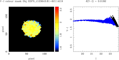
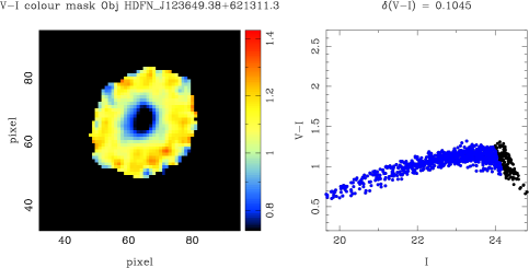
Figure 1: The methodology of internal colour variations as applied to two HDF-N spheroidals. The upper panel shows an $I_{814}=20.48$ mag example with low internal scatter at $z=0.77$, whereas the bottom panel illustrates an $I_{814}=21.66$ example with a bluer core at $z=0.48$. The pixel-by-pixel colour distributions are shown alongside each case. Coloured dots refer to pixels whose SNR is above the adopted threshold.

Initially we will focus on a largely model-independent approach to the problem of understanding how the internal colours of field ellipticals vary with redshift relative to those of their clustered counterparts. We will concentrate only on $I_{814}$ and $V_{606}$  bands, as the resulting $V_{606}-I_{814}$ colours have substantially smaller observational errors than the $B_{450}-V_{606}$ and $U_{300}-B_{450}$ colours, especially for systems dominated by old stellar populations.

3.1.1 The Homogeneity Estimator

Figure 2: The observed $\delta(V-I)$ as a function of redshift for modelled galaxies viewed at various redshifts with two photometric colour systems. The $V_{606}-I_{814}$ (solid lines) and $V_{555}-I_{814}$ (dashed line) curves are plotted for two cases: a single-burst (“Passive”) system corresponding to an epoch of formation $z_{F}=5$, and an “Active” case which incorporates a 15% by mass burst of star formation centrally super-imposed on an old galaxy at the time of observation.

After registering the Northern HDF images to sub-pixel accuracy, we isolated each galaxy from the background sky by selecting all contiguous pixels within a surface brightness threshold of $V_{606}=25.5$ mag arcsec^-2. We select this limit in order to maximize the signal/noise per pixel associated to $V_{606}-I_{814}$ colours.

The distribution of $V_{606}-I_{814}$  colours for individual pixels in the galaxy is used to calculate a quantity $\delta(V-I)$ which characterises the internal homogeneity of a galaxy. A $\delta(V-I)$ statistic is defined as:

$$\delta(V-I)=2N\frac{\sum(x_{i}-\bar{x})^{2}S(x_{i}){\mathit{SNR}}(x_{i})}{\sum S(x_{i}){\mathit{SNR(x_{i})}}}$$ (1)

$$\bar{x}=\frac{\sum x_{i}S(x_{i}){\mathit{SNR}}(x_{i})}{\sum S(x_{i}){\mathit{SNR}}(x_{i})}$$ (2)

where $S(x)$ is a selection function for pixels with signal/noise above a certain threshold ($SNR>1.3$) such that $S(x)=1$ for pixels above and $S(x)=0$ for pixel below the threshold. $SNR(x_{i})$ is the signal-to-noise ratio for a given pixel colour $x_{i}$, and $N$ is an arbitrary scale factor. The selection function $S(x)$ and the weighting according to $SNR(x)$ address biases arising from noise variations at pixel scales by rejecting low signal pixels and weighting the pixels contribution proportionally to their signal. Figure 1 show an example of spheroidals in HDF-N with both high and low $\delta(V-I)$ .

As mentioned previously, the MORPHS dataset was observed with a different filter baseline than that used for the HDF. To quantify the effect of this difference on $\delta(V-I)$, we used stellar population synthesis libraries (Bruzual & Charlot 1996, BC96) to calculate the observed colours (in both photometric systems) for two galaxy types: a) an old single-burst elliptical (formation epoch $z_{F}=5$ and $e$-folding time $\tau=1$ Gyr) and, b) a star-forming elliptical galaxy consisting of a recent burst ($100$ Myr) centrally superimposed on an old system. In order to emulate the geometrical properties of the modelled galaxies, we use the observed colours at a given redshift to create elliptical galaxies with $r^{1/4}$ profiles using a customised version of the IRAF package artdata and a fixed physical size with a half-light radius $r_{e}=2.5$ kpc. For the case of the blue core, we attempt to match the properties of Figure 1 lower panel, with a burst that accounts for 15% of the total mass of the galaxy with and a physical size of $0.1r_{e}$. $\delta(V-I)$ for both photometric systems are shown as a function of redshift in Figure 2. This exercise demonstrates that the substitution of F555W for F606W does not have a major impact on the calculation of $\delta(V-I)$ . The slightly longer wavelength baseline in the cluster $\delta(V-I)$ estimates should result in a greater sensitivity to recent activity.

It is important to note that because $\delta(V-I)$ is based on observed (rather than rest-frame) colours, its sensitivity to star formation is redshift-dependent. Unfortunately, it is not possible to use additional filters to create a rest-frame equivalent since the shorter wavelength HDF data has poorer signal/noise and the cluster data only consists of two passbands. In order to quantify this restriction, we studied values of $\delta(V-I)$ obtained for the blue core case modelled in Figure 2. We placed this modelled galaxy, at the epoch corresponding to its maximum inhomogeneity (representing the most extreme case we will discuss) at various redshifts calculating $\delta(V-I)$ at each redshift. Figure 2 shows increased sensitivity to the fixed star formation rate at $z\sim 0.5$ for F606W and $z\sim 0.4$ for F555W; otherwise the sensitivity is broadly constant. This increase arises as the 4000Å  break in the underlying passive system passes through the F606W and F555W filters and will not seriously compromise our analysis.

3.1.2 The Influence of the HST Point-Spread Function

Figure 3: The colour inhomogeneity $\delta(V-I)$ for real and simulated data sets as a function of their central concentration indicating the level of bias introduced by the wavelength-dependence of the HST point spread function.

As the HST point-spread function (PSF) varies as a function of wavelength, spurious centrally-concentrated inhomogeneities might be expected for sharply-peaked profiles such as those encountered in spheroidal galaxies. In order to test this, we performed extensive Monte Carlo simulations using the Iraf package artdata. Artificial galaxy images were created and subsequently analysed using procedures identical to those used to analyse our observed data.

Artificial spheroidal galaxies were synthesised with de Vaucouleurs profiles, using stars from the HDF-N as PSF templates. Simulated images were generated in both $I_{814}$ and $V_{606}$ –bands. We explored a range of half-light radius ($r_{e}$) from $0.04^{\prime\prime}-0.65^{\prime\prime}$ corresponding to $\sim 0.4-6$ kpc ($H_{0}=65$ km s^-1 Mpc^-3, $q_{0}=0.1$), and a range of magnitudes representative of our sample ($18<I_{814}<24$ mag). As the influence of the PSF on the central colours is expected to be a strong function of the “peakiness” of the central portion of the galaxy, we chose to probe the influence of the PSF on both real and simulated galaxies as a function of the central concentration ($C$) parameter defined in Abraham et al. (1994).

Figure 3 shows the result of this exercise. The PSF variations affects the $\delta(V-I)$ statistic only for the most centrally concentrated (essentially stellar) objects. Over the observed range of C for the real data, $0.3\lower 2.15277pt\hbox{$\;\buildrel<\over{\sim}\;$}C\lower 2.15277pt\hbox{$\;\buildrel<\over{\sim}\;$}0.7$, $\delta(V-I)$ in the simulated data is well below the values recovered from the real observations, and we conclude that this effect will not seriously affect any of the following conclusions.

3.2 Evolution in Field Spheroidals

Figure 4 shows $V_{606}-I_{814}$ colour maps for the 79 spheroidals in our HDF sample sorted in ascending order according to $I_{814}$ magnitude. Redshift and $\delta(V-I)$ values are also marked in each case; redshifts in parenthesis refer to photometric estimates. The most striking characteristic of these data is the large proportion with significant internal colour variations. We emphasise that we have not significantly varied the ”colour stretch” from panel to panel (as indicated in the colour bar) to exaggerate this result. Adopting, for simplicity, a colour variation of $\simeq 0.2$ mag as indicative of the effect (since this broadly corresponds to a change in visual colour according to our look-up table), it appears that $\sim 40\%$ of the field spheroidals show a detectable degree of inhomogeneity. In most cases where inhomogeneities are seen, these appear to be in the cores. Obviously, the visual inhomogeneities correlate closely with $\delta(V-I)$ .

In § 3.3 we will calibrate these inhomogeneities with reference to a corresponding sample of cluster spheroidals, but it is meanwhile interesting to consider whether these internal colour variations correlate with independent constraints. In doing this we will make the assumption that the bluer colours seen are indicative of recent star formation.

Figure 4: Colour images of 79 HDF field spheroidals keyed to their $V_{606}-I_{814}$ colours. The integrated $I_{814}$ mag for each galaxy is shown in each sub-panel together with the redshift and $\delta(V-I)$ . Redshifts in parenthesis indicate photometric estimates. Axes labels correspond to arcseconds

Figure 5: continued

3.2.1 Comparison with Kodama et al.

Figure 6: The distribution of $\delta(V-I)$ with redshift for those HDF spheroidals studied by Kodama et al. (1998, KBB). The size of the symbols indicates the $I_{814W}$ integrated magnitude.

We first compare our $\delta(V-I)$ estimates with the results of Kodama, Bower & and Bell (1998, KBB). Those authors used stellar population models and photometric redshifts to construct a rest-frame $U-V$ vs. $V$ colour-magnitude diagram for field spheroidals in the HDF-N. They took the morphologically-classified sample of 35 spheroidals with $K<20.5$ from Franceschini et al. (1998) of which 29 are in our sample. The 6 missing cases correspond to two classes of objects: a) objects that only Franceschini et al. classified as spheroidals, and b) double detections in the Franceschini et al. (1998) study which we have eliminated. Using spectral synthesis models, KBB concluded that the sample could be described as comprising a red sequence of old passively-evolving systems, with an additional component (comprising 30% of the total sample) with bluer optical-infrared colours that lay significantly off the fiducial colour-magnitude relation.

We have divided the Franceschini et al. subsample of our HDF-N spheroidals into ’red’ and ‘blue’ examples depending on whether their rest-frame colours lie within the red sequence limits defined by KBB. Specifically, we classed as blue all spheroidals whose rest-frame colours have $U-V<0.8$. Figure 6 compares our $\delta(V-I)$ with the red/blue classifications demonstrating a strong correlation with the estimated $U-V$ rest-frame colour from KBB. In all but one case, red KBB spheroidals correspond to low $\delta(V-I)$ systems in our scheme. We estimate that $\sim 9$ out of of 29, or $\sim 30$% of spheroidals have values of $\delta(V-I)$ suggesting some degree of star-formation activity, a value in excellent agreement with the KBB estimate.

The strong correlation between our model-independent measures of $\delta(V-I)$ and KBB’s estimates of rest-frame $U-V$ is reassuring evidence that simple spectral synthesis models used to describe spheroidal evolution offers a valid way to quantitatively interpret our results. Armed with this reassurance, in §4.2 we will use similar models to attempt to constrain the amount of star-formation contributed by evolving spheroidals as a function of redshift.

3.2.2 Low $\delta(V-I)$ field spheroidals

Despite the significant fraction of spheroidals showing some degree of colour variation, the majority show homogeneous internal colours, suggesting coeval evolution of their stellar populations. We selected the galaxies with low $\delta(V-I)$ $\leq 0.04$ and compared their integrated colours against the predictions of a monolithic collapse model. As expected this sample closely tracks the expected colour-redshift relation of a passively evolving (Figure 7) providing reassurance that $\delta(V-I)$ is a good statistic from which to differentiate active and passive systems.

An interesting feature is the somewhat larger fraction of homogeneous spheroidals within HDF-N with respect to the HDF-S. Only 4 spheroidals in the HDF-S show low $\delta(V-I)$ values compared to 15 spheroidals in the HDF-N. This could be interpreted as evidence for clustering in the HDF-N as suggested by Kodama et al. (1998).

Figure 7: The $V_{606}-I_{814}$ observed colours for a subsample of internally homogeneous ($\delta(V-I)$ $\leq 0.04$) spheroidals as a function of redshift compared with the predictions of a high-redshift single burst model ($z_{F}=5$, $\tau=1$ Gyr) and solar metallicity for a set of cosmologies. Inverted triangles refer to HDF-S and unfilled symbols refer to galaxies for which only photometric redshifts are available.

3.3 Evolution in Cluster Spheroidals

As we discussed in $\S$1, it is now commonly-believed that spheroidals in the cores of rich clusters formed the bulk of their stars before $z\lower 2.15277pt\hbox{$\;\buildrel>\over{\sim}\;$}2$ (Bower et al. 1992, Ellis et al. 1997, Governato et al. 1998, Kauffmann et al. 1999). Cluster samples therefore represent suitable benchmarks whose $\delta(V-I)$ values at a given redshift can be used to provide a model-independent calibration of the internal colour scatter expected from an old stellar population at a given redshift.

As mentioned earlier, our limiting magnitude in the cluster sample was chosen as $I_{814}=22$, considerably brighter than adopted for the deeper HDF images. The morphological classifications were taken from the published articles. In the case of the MORPHS sample there is a cross-check given one of us (RSE) classified both samples. As in the previous section we have calculated $\delta(V-I)$ for each cluster spheroidal using the prescription given in equation 2. We find a striking absence of internally inhomogeneous systems. In fact, we find no cluster spheroidals with blue cores in any of the five clusters. We then calculate a median $V_{606}-I_{814}$ value and will take this as representative of the $\delta(V-I)$ value appropriate for an old spheroidal population over the redshift range $0.37<z<0.83$ (Figure 8).

Figure 8: Mean $\delta(V-I)$ values and $1\sigma$ dispersions calculated for spheroidal galaxies in 5 clusters observed with HST in similar passbands to those used for the HDF field study.

Figure 9: $\delta(V-I)$ values for the HDF-N and HDF-S spheroidals compared with their clustered counterparts as a function of $M_{450}$ absolute magnitude for three redshift ranges. Solid points represent cluster galaxies and open ones field spheroidals.

The strongest result of this paper is that field spheroidals show substantially greater internal colour dispersions than their clustered counterparts. Since the limiting magnitude of the field sample is two magnitudes brighter than that adopted for the cluster sample, this is most cleanly demonstrated by comparing $\delta(V-I)$ values on a galaxy-by-galaxy basis in both samples as a function of rest-frame luminosity (Figure 9). Absolute magnitudes were calculated assuming $H_{0}=65$ km s^-1 Mpc^-1. In the cluster analysis, galaxies smaller than 60 pixels were not considered, as the $\delta(V-I)$ measurement was determined to be too noisy to be meaningful. Although about 15% of the cluster spheroidals were rejected on this basis, from Figure 9 we are reassured that we are probing a similar range of $M_{B450}$ absolute magnitudes.

For the cluster spheroidals we calculated $M_{B450}$ for each galaxy from its $I_{814}$ apparent magnitude by applying K-corrections and colour terms based on a high-redshift single-burst model ($z_{F}=5,\tau=1$ Gyr) which, as we have discussed, reproduces the observed colours (Bower et al. 1992, Ellis et al. 1997). For the field spheroidals we computed $M_{B450}$ using $B_{450}$ apparent magnitudes, given in version 2 of the HDF SExtractor catalogues, and a maximum likelihood method describe more fully in $\S$4.2. Anticipating this discussion, briefly the method allows us to obtain the most-likely K-correction for each individual pixel within the galaxy. This complication is necessary given the hybrid nature of the spectral energy distribution in the internally inhomogeneous cases.

Clearly, over similar ranges of absolute magnitudes, field spheroidals show markedly larger dispersions in their internal colours than do cluster spheroidals. Although cluster spheroidals have more homogeneous internal colours, there is a trend for $\delta(V-I)$ to grow as a function of redshift. The trends calculated in Figure 2 shows that this is not an artifact relating to a greater sensitivity to very small amounts of star formation. Unfortunately the limited depth of the cluster data does not allow us to put more meaningful constraints on the evolution of the cluster population.

4 SPECTRAL SYNTHESIS MODELLING OF INTERNAL COLOUR VARIATIONS

Simple comparisons between the internal colour distributions of field and cluster samples allow us to establish, in a model-independent way, the proportion of active systems as a function of redshift and environment. Given that detailed spectroscopic information is not yet available for the sample, in order to learn more about the relevant timescales for the presumed star formation activity we must now turn to more detailed synthesis models. In this section we will investigate how simple models can be used to place broad constraints on the buildup of mass implied by the internal colour variations reported in this paper.

4.1 A Simple Evolutionary Model For Field Spheroidals

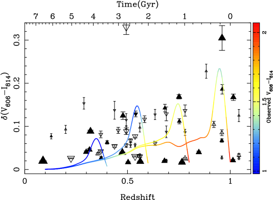
Figure 10: The observed $\delta(V-I)$ predicted for the blue-nucleated model spheroidal (solid line) compared with observed values in the HDFs. The colour gradient along the evolutionary track maps the observed evolution in $V_{606}-I_{814}$ according to the right hand scale bar. Error bars in the field spheroidals show the $1\sigma$ deviation obtained from 100 bootstrap resamplings of the data pixels within each galaxy and field symbols follow the designations of Figure 6.

The blue light in field spheroidals reported in the present paper arises, in the majority of cases, in the central regions. Possible origins include residual star-formation from a recent major merger (Kauffmann 1996), low-level star-formation that is a relic from a high-redshift collapse (Jiménez et al. 1999), cooling flows from hot gas surrounding the central region of the ellipticals, or a bursts of central star-formation possibly related to the inflow of gas arising from a recent minor merger. In this section we aim to place constraints on the star-formation timescales and masses associated with the activity we claim to observe predominantly in the field population. We do this within the context of a simple model that seeks to reproduce the observed spatially resolved colours of the subset of active ellipticals with prominent blue nuclei.

We assume that an intermediate redshift field spheroidal can be described with a two component model – an old underlying stellar component which formed at high redshift and a secondary younger component (responsible for the central blue light). The integrated colours of both components are estimated using the stellar population synthesis library of Bruzual & Charlot (1996, BC96). We modelled the old component using a 1 Gyr exponentially declining burst of star formation commencing at a redshift of formation $z_{F}=5$. We adopt a flat Universe with $\Omega_{0}=0.3$, $\Omega_{\Lambda}=0.7$. The secondary population is modelled via an additional instantaneous burst of star-formation presumed to occur close to the epoch of observation. The present modelling is similar to the one described in $\S$ 3.1.1, however here we include the evolution as function of the galaxy age.

In order to mimic the resolved properties of a model galaxy, we create an image of the two galaxy components using a modified version of IRAF mkobjects. For the old component we use a de Vaucouleurs profile with a half-light radius of $r_{e}=2.5$ kpc. For the central blue component we also use a de Vaucouleurs profile, but with an effective radius $0.1r_{e}$. We assume 15% of the galaxy mass is in the young component, and that the total mass is $M=1\times 10^{12}$ M_☉. Finally, between $0<z<z_{burst}$ we combine the two components by adding up the images using the colours predicted by our spectral synthesis models. For the resulting galaxy we calculate $\delta(V-I)$ and repeat the procedure four times corresponding to 15% (by mass) bursts at redshifts $z_{burst}=$ 1.0, 0.8, 0.6 and 0.4.

Figure 10 shows the result of this exercise, superposed on the observed $\delta(V-I)$ for the HDF spheroidals. Error bars correspond to $1\sigma$ estimates obtained by bootstrapping the data as described in Efron & Tibshirani (1986). We conclude that our simple model can successfully reproduce the range of observed $\delta(V-I)$ as well as the observed increase $\delta(V-I)$ with redshift. The essential point is that the observed internal colour scatter is not necessarily a relic of the initial elliptical formation event and can quite easily represent a perturbation introduced by a recent episode of star-formation (forming only a modest proportion of the total stellar mass) superposed on a pre-existing old population. If this is the case then excursions from the homogeneous colours of the underlying old stellar population are probably brief, lasting about 1 Gyr after which the galaxy returns to its pre-burst value. Ultimately high resolution spectra of large sample of spheroidals using Balmer lines will enable us to disentangle the internal clock of star formation for field spheroidals. However from this simple study it seems reasonable to conclude that as many as half the field spheroidal population share this activity by $z\sim 1$.

4.2 The Star Formation History of Spheroidals

If our interpretation of Figure 10 is correct, the question arises as to the extent of this recent activity in terms of the evolution of global star formation and its role for the mass assembly of field spheroidals as predicted in popular hierarchical models. Although the HDF samples are very modest ones on which to base such fundamental studies, we explore these wider issues using the analytical techniques described in Abraham et al. (1999).

In the HDF-N, Abraham et al. were able to reconstruct a simple cosmic star-formation history by interpreting resolved multi-colour data in the context of evolutionary synthesis models. For each HDF galaxy, an integrated star formation rate was determined and volume-averaged values ($\rho_{\mathrm{S}FR}$ ) for the entire population was derived using a simple $V/V_{max}$ methodology. Here we will attempt to estimate the contribution to $\rho_{\mathrm{S}FR}$ arising from our HDF spheroidals and compare its evolutionary decline with time with that observed in other morphological populations. The crucial advantage of an analysis utilising the resolved colours is that it enables a determination of the relative ages and star-formations of the components within the galaxies.

4.2.1 The Method

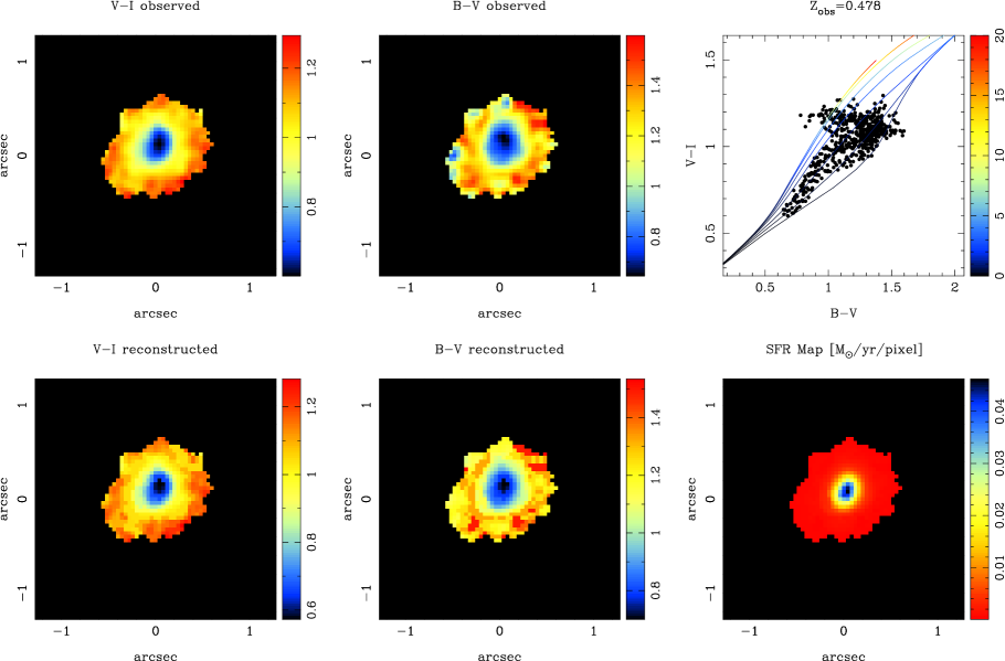
Figure 11: A demonstration of our maximum likelihood methodology showing the observed and reconstructed $V_{606}-I_{814}$ and $B_{450}-V_{606}$ colours. The reconstructed colours and SFR (lower right) maps were based on the the best fit models to the pixel colour-colour diagram (upper right). The colour assigned to the tracks drawn in the colour-colour diagram indicates age in Gyr according to the right hand colour bar (blue=young, red=old). As expected, the blue core is a region of current star formation, whereas the outer region shows virtually no activity.

Using the precepts of Bruzual & Charlot (1991), the total flux from a stellar system, $F_{\lambda}$ observed at an age $t_{0}$ can be described as the convolution of the spectrum of an evolving instantaneous burst, $f_{\lambda}(t)$, with an star-formation history given by $\Psi(t)$.

$$F_{\lambda}(t_{0})=\int_{0}^{t_{0}}\Psi(t_{0}-t)f_{\lambda}(t)dt$$ (3)

In our analysis, we use the stellar population synthesis libraries from gissel96 (Bruzual & Charlot 1996) to estimate $f_{\lambda}$, assuming a Scalo IMF with lower and upper limits of 0.1 and 125 M_☉ respectively and solar metallicity. For the SFR function $\Psi(t)$, we assume that the colours of a given stellar population can be modeled by exponential star-formation histories with a characteristic time-scale $\tau$ of the form,

$$\Psi(t)=\Psi_{0}e^{-t/\tau}.$$ (4)

which enables us to describe a wide range of star-formations, given that $\tau\to\infty$ approximates a constant star formation, while $\tau\to 0$ approximates an instantaneous burst.

As the $U_{300}$-band flux is weak for our sample, adding this to the analysis would enlarge the uncertainties in the observed colours of spheroidals rather than further constrain our estimates. Therefore, we concentrate on the $B_{450}$, $V_{606}$, and $I_{814}$ bands only. We calculate the $B_{450}-V_{606}$ vs $V_{606}-I_{814}$ evolutionary tracks as observed at the galaxy redshift for a set of representatives formation histories ($\tau=0.1$, 0.2, 0.4, 1, 2, 4, and 9 Gyr) using the stellar population libraries from gissel96. For each spheroidal, we select all the contiguous pixels within a surface brightness threshold of $B_{450}=26$ mag/arcsec², and from the selected pixels construct the corresponding $B_{450}-V_{606}$ vs $V_{606}-I_{814}$ colour-colour diagram for each of the galaxies. We define this limit in order to maximize the signal/noise associated per pixel in both the $B_{450}-V_{606}$ and $V_{606}-I_{814}$ colours, selecting in the lowest signal band in order to ensure an uniform signal criteria in the pixel selection. We estimate the optimum model and age for each pixel using a maximum likelihood estimator ${\cal L}$ defined as:

$${\cal L}(t,\tau)=\prod_{i=1}^{2}{1\over\sqrt{2\pi}\delta C_{i}}\exp\left(-{(c_{i}-C_{i})^{2}\over 2\delta C_{i}\,^{2}}\right)$$ (5)

where we take the product over both colours $B_{450}-V_{606}$ and $V_{606}-I_{814}$ , $C_{i}$ and $\delta C_{i}$ represent the data colour and colour error associated with the pixel respectively, and $c_{i}$ is the colour of the modelled track at a given age and e-folding time-scale $\tau$. For each pixel we obtain the most likely age, SFR and $\tau$ value. Repeating over all acceptable pixels, we obtain the integrated value at the observed redshift. This procedure is repeated for all spheroidals in the HDFs. In order to illustrate this methodology, in Figure 11 we show a typical pixel-by-pixel colour-colour diagram and illustrate how the predicted evolutionary tracks at the redshift of observation can reconstruct the $V_{606}-I_{814}$ and $B_{450}-V_{606}$ observed colours and construct a SFR map for each galaxy pixel.

Given that our methodology depends explicitly on the redshift of the galaxy, we need to take into account the uncertainties associated with the photometric estimates when calculating SFR for galaxies with photometric redshifts. Up to $z\sim 1$, photometric redshifts have proved to be in reasonable good agreement with spectroscopic redshifts with an rms error of $\delta z\sim 0.1$ for red populations (Hogg et al. 1998, Gwyn et al. 2000, de Soto et al. 1997). We performed Monte Carlo simulations by refitting each galaxy using the models for the appropriate photometric redshift plus a random component of $\delta z=0.1$. Repeating this exercise for each galaxy with photometric estimates allows us to obtain an uncertainty on the total SFR estimated for those systems for which only photometric redshifts are available.

Clearly the predictions of spectral synthesis models are sensitive to both metallicity and dust content, neither of which is well constrained in our data. The presence of dust would have the effect of underestimating the computed SFR, whereas metallicity changes will produce systematic shifts between the predicted age and colours of each galaxy. Whilst recognising the limitations involved, our primary goal at this stage is to illustrate the potential of our resolved colour technique to determine redshift-dependent trends rather than to derive precise absolute values. Throughout the SFR analysis we will use solar metallicity in our calculations, as from Figure 7 we can see that this reproduces fairly well the observed colour of low $\delta(V-I)$ spheroidals. With resolved infrared data such as may be available from NICMOS, it may ultimately be possible to limit the uncertainties arising from dust.

4.2.2 Evolution in the Star-Formation density of spheroidals

We now estimate the SFR density ($\rho_{\mathrm{S}FR}$) of spheroidals as a function of redshift and choose to compare these estimates with similar ones derived for a parallel sample of morphologically-irregular galaxies in both HDFs. In the case of the latter, we used the morphological classification of Abraham et al. and adopted the same $I_{814}$ limit for both HDFs.

Figure 12: The comoving SFR density computed using the 63 spheroidal (filled circles) and 51 morphologically-irregular (filled stars) galaxies in both HDFs. Corrections for incompleteness were made assuming SFR $\propto L$, local luminosity functions and evolutionary corrections described in the text. Hollow symbols represent uncorrected values. Error bars take into account systematic uncertainties implied in the calculation of the SFR in individual galaxies and bootstrap errors which account for the small sample size.

We calculate the SFR density at a given redshift interval $z_{1}<z<z_{2}$ using the expression,

$$\rho_{\mathrm{S}FR}(z)=\sum_{i;z_{1}<z_{i}<z_{2}}\frac{{\mathit{S}FR}_{i}}{V_{max,i}}$$ (6)

where the sum is over all the galaxies $i$ for which $z_{1}<z_{i}<z_{2}$ and $V_{max}$ is the volume at $z_{max}$, the largest redshift at which the galaxy $i$ remains brighter than our limiting magnitude (Schmidt 1968). Clearly as we move towards higher redshifts our sample becomes increasingly biased towards intrinsically more luminous galaxies and we will consequently neglect a contribution to $\rho_{\mathrm{S}FR}$ from sub-luminous objects. To correct for this we need to assume: i) the dependence of the SFR on the luminosity $L$, ii) the shape of the spheroidal luminosity function and iii) the luminosity evolution assumed for the spheroidal population. Whilst none of these is unfortunately known precisely, we can make progress by assuming that $\mathit{SFR}\propto~{}L$ (i.e. the most luminous galaxies form the most stars) and adopting a suitable Schechter luminosity function (LF). Under these assumptions, the corrected SFR density ($\tilde{\rho}_{\mathrm{S}FR}$) would become:

$$\tilde{\rho}_{\mathrm{S}FR}(z)=C(z)\rho_{\mathrm{S}FR}(z)$$ (7)

with,

$$C(z)=\frac{\int_{0}^{\infty}{\mathit{SFR(L)}}\phi(L)dL}{\int_{L_{min}}^{\infty}{\mathit{SFR(L)}}\phi(L)dL}=\frac{\Gamma(\alpha+2)}{A}$$ (8)

and,

$$A=0.4\ln(10)\int_{-\infty}^{M^{-}}10^{0.4(M^{\star}-M)(\alpha+2)}e^{-10^{0.4(M^{\star}-M)}}dM$$ (9)

where $M^{\star}$ may be permitted to evolve with redshift (e.g. according to an evolutionary correction) and $M^{-}$ and $L_{min}$ are the faintest absolute magnitudes and luminosities respectively within the redshift interval in question.

As an illustration of the technique, we adopted Schechter LFs from Marzke et al. (1998) with $M^{\star}_{b_{j}}=-20.87$ and $\alpha=-1$ for the HDF spheroidals and $M^{\star}_{b_{j}}=-21.28$ and $\alpha=-1.81$ for the irregulars. For the spheroidals we assumed $M^{*}$ evolves according to that appropriate for a passively evolving system with ($\tau=1$ Gyr). In the case of the irregulars, we assumed a constant SFR ($\tau=5$ Gyr).

Finally is necessary to define a number density correction factor, ${\cal K}(z)$, very similar to the one described in equation 8 to estimate the redshift completeness of our sample, viz.

$${\cal K}(z)=\frac{\Gamma(\alpha+1)}{B}$$ (10)

and

$$B=0.4\ln(10)\int_{-\infty}^{M^{-}}10^{0.4(M^{\star}-M)(\alpha+1)}e^{-10^{0.4(M^{\star}-M)}}dM$$ (11)

where $M^{-}$ is the faintest absolute magnitude included in the sample at a given redshift determined by our flux limit of $I_{814}=24$ mag and the distance modulus relation.

Although ${\cal K}(z)$ and $C(z)$clearly depend on the poorly-constrained LF shape, for our adopted values we find completenesses (in terms of the contribution of detectable galaxies to the integrated $\rho_{\mathrm{S}FR}$ ) of $\sim 90\%$ and $\sim 80\%$ for 63 HDF spheroidal and 51 HDF morphologically-irregular galaxies respectively.

Figure 12 shows the results of our calculations and the uncertainties introduced by our corrections for incompleteness. As expected these corrections become more important at higher redshifts and for the morphologically-irregular population whose LF is presumed to be steep at all times ($\alpha<-1$). However in most of the cases the corrections are comparable to the size of the statistical uncertainties. Random errors bars were calculated by adding in quadrature the systematic errors in the SFR calculation for individual galaxies, including the Monte Carlo estimates for the photometric redshift and Poisson errors estimated by bootstrapping 100 times the sample when computing the SFR density. In Table 2 we list the computed values for $\rho_{\mathrm{S}FR}$ as well as their uncertainties.

Figure 12 enables us to provide the first rough constraints on the contribution of the increased colour variation in the HDF spheroidals to the evolution of the $\delta(V-I)$. A rise with redshift is discernible but the uncertainties are considerable. Interestingly, the evolution in $\rho_{\mathrm{S}FR}$ mirrors, but at a lower level, that established more convincingly for field irregulars from the CFRS/LDSS sample of Brinchmann et al. (1998) (but estimated here for the HDF from a completely independent resolved colour method). Brinchmann et al. computed $\rho_{\mathrm{S}FR}$ between $0.3<z<0.9$ using the equivalent width of [Oii]. Although their $\rho_{\mathrm{S}FR}$ values are systematically lower for both the spheroidal and peculiar/irregular population, similar evolutionary trends were observed in the overlapping redshift range $0.4<z<1.0$. If it could be established that the decline in the spheroidal $\rho_{\mathrm{S}FR}$ was driven by that associated with the demise of the more active irregular population, this would provide further support that the blue cores observed in the HDF spheroidals arise from recent mergers of the irregular population (Le Fèvre et al. 1999, Brinchmann 1999, Brinchmann & Ellis 2000).

Table 2: SFR density estimates

Redshift	Spheroidalsuncorrected	Spheroidals${}^{a}_{corrected}$	Irr/Pecuncorrected	Irr/Pec${}^{b}_{corrected}$
0.15	$-3.642^{-2.956}_{-4.329}$	$-3.641^{-2.954}_{-4.328}$	$-2.948^{-1.001}_{-4.895}$	$-2.766^{-1.896}_{-3.636}$
0.45	$-2.615^{-2.348}_{-2.881}$	$-2.609^{-2.342}_{-2.875}$	$-2.020^{-1.685}_{-2.354}$	$-1.752^{-1.417}_{-2.087}$
0.75	$-2.581^{-2.195}_{-2.966}$	$-2.563^{-2.177}_{-2.949}$	$-1.688^{-1.176}_{-2.201}$	$-1.285^{-0.772}_{-1.797}$
1.05	$-2.106^{-1.520}_{-2.692}$	$-2.070^{-1.484}_{-2.656}$	$-1.442^{-1.010}_{-1.873}$	$-0.883^{-0.452}_{-1.314}$

5 CONCLUSIONS

We have exploited HST’s unique capabilities to resolve distant galaxies by examining the internal colour distribution of a sample of 79 field spheroidals in both Hubble Deep Fields. From a model-independent analysis of our data, we find:

$\bullet$ A significant fraction ($>$30%) of field spheroidals show marked variations in their internal colours. In most of the cases where colour variations are seen, this manifests itself in terms of centrally-located blue cores.

$\bullet$ Using a statistic, $\delta(V-I)$, to characterise the internal homogeneity of a galaxy we have extended our analysis to permit a comparison of the internal variations found in the HDF sample with that for a sample of spheroidal galaxies in five rich clusters spanning a similar redshift range. Marked differences are found in the sense that galaxies of the same luminosity and redshift are consistently more uniform in rich clusters than in the field. Assuming the blue colours located in the HDF field ellipticals arise from recent star formation, our comparison provides strong evidence for more extended star formation histories in field ellipticals (as expected in hierarchical models).

$\bullet$ We compare our observational diagnostics with those used by other workers and find general agreement. The most straightforward interpretation of our data is that a fraction of field spheroidals at intermediate redshift has undergone recent star formation, perhaps as a result of recent merging or an inflow of material.

Using spectral synthesis models and a maximum likelihood analysis developed by Abraham et al. (1999) we attempt to reproduced the observed colour variations for the field spheroidals and to compute their current SFR. From this model-dependent analysis we find that:

$\bullet$ Assuming that the observed blue nuclei observed in some field spheroidals arises from a recent burst of star-formation superposed on a pre-existing old stellar population, we can readily reproduce the observed distribution of $\delta(V-I)$ values. The star formation episodes implied are short, lasting less that 1 Gyr, and typically involve 15% of the galactic mass.

$\bullet$ If the HDF fields are representative, the fraction of field ellipticals undergoing activity of this kind could be as high as $\sim 50\%$ at $z\sim 1$.

$\bullet$ The contribution to the global SFR density from field spheroidals, whilst uncertain to determine accurately because of the necessary corrections for incompleteness and possible luminosity evolution, appears to rises modestly as a function of redshift in a manner which may connect with the demise in activity associated with morphologically-irregular systems.

With a larger sample, augmented with diagnostic spectroscopy capable of constraining the timescale of recent activity, it may be possible to strengthen the connection between the declining luminosity density contributed by morphologically-irregular galaxies and the implied continued assembly of field ellipticals. The goal remains an important one in understanding the origin of the Hubble sequence and in defining the role of the environment (Brinchmann & Ellis 2000).

References

- [Abraham, et al. (1999)] Abraham, R. G., Ellis, R. S., Fabian, A. C., Tanvir, N. R. & Glazebrook, K. 1999, MNRAS , 303, 641.
- [Abraham et al. 1996] Abraham, R. G., van den Bergh, S., Ellis, R. S., Glazebrook, K., Santiago, B. X., Griffiths, R. E., Surma, P. 1996, ApjSS, 107, 1.
- [Abraham et al. 1994] Abraham, R. G., Valdes, F., Yee, H. K. C., and van den Bergh, S., 1994, ApJ, 432, 75.
- [Baade 1957] Baade, W. 1957 in Stellar Populations, ed. O’Connell, D.J.K. p3, Vatican (Rome).
- [Barger et al. 1998] Barger, A. J., Cowie, L. L., Trentham, N., Fulton, E., Hu, E. M., Songalia, A. & Hall, D., 1998, AJ 117, 102.
- [Baugh et al. 1996] Baugh, C. Cole, S. & Frenk, C.S. 1996 MNRAS 283, 1361.
- [Bower et al. 1992] Bower, R.G., Lucey, J.R. & Ellis, R.S. 1992 MNRAS 254, 601.
- [Brichmann & Ellis 2000] Brinchmann, J. & Ellis, R. S. 2000, ApJL submitted.
- [Brinchmann Thesis] Brinchmann, J. PhD Thesis, 1999, Cambridge University.
- [Brinchmann, et al. (1998)] Brinchmann, J. , et al. 1998, ApJ , 499, 112.
- [BC96] Bruzual, G. & Charlot, S. 1996 (BC96).
- [Efron & Tibshirani 1996] Efron, B., & Tibshirani, R. 1986, Statistical Science, 1, 1, 54.
- [Ellis et al. 1997] Ellis, R.S. Smail, I., Dressler, A. et al, 1997 ApJ, 483, 582.
- [Fernández-Soto, Lanzetta Yahil (1999)] Fernandez-Soto, A. , Lanzetta, K. M. & Yahil, A. 1999, ApJ , 513, 34.
- [Franceschini, et al. (1998)] Franceschini, A. , Silva, L. , Fasano, G. , Granato, L. , Bressan, A. , Arnouts, S. & Danese, L. 1998, ApJ , 506, 600.
- [Governato, et al. (1999)] Governato, F. , Gardner, J. P., Stadel, J. , Quinn, T. & Lake, G. 1999, AJ, 117, 1651.
- [Hogg, et al. (1998)] Hogg, D. W., et al. 1998, AJ, 115, 1418.
- [Jiménez, et al. (1999)] Jiménez, R. , Friaca, A. C. S., Dunlop, J. S., Terlevich, R. J., Peacock, J. A. & Nolan, L. A. 1999, MNRAS, 305, L16.
- [Kauffman et al. 1996] Kauffmann, G., Charlot, S. & White, S.D.M. 1996 MNRAS 283, L117.
- [Kauffmann, Colberg, Diaferio White (1999)] Kauffmann, G. , Colberg, J. M., Diaferio, A. & White, S. D. M. 1999, MNRAS , 303, 188.
- [Kodama, Bower Bell (1999)] Kodama, T. , Bower, R. G. & Bell, E. F. 1999, MNRAS , 306, 561 (KBB).
- [Le Fèvre, et al. (2000)] Le Févre, O., et al. 2000, MNRAS , 311, 565.
- [Marleau Simard (1998)] Marleau, F. R. & Simard, L. 1998, ApJ, 507, 585.
- [Madau et al. 1998] Madau P., Pozzetti L., & Dickinson M., 1998, ApJ, 498, 106.
- [Menanteau et al. 1999] Menanteau, F., Ellis, R. S., Abraham, R. G., Barger, A. J., & Cowie, L. L. 1999 MNRAS, 309, 208.
- [Sandage 1986] Sandage, A. 1986 in Deep Universe, ed. Binggeli, B. & Buser, R. p1, Springer-Verlag (Berlin).
- [Smail et al. 1997] Smail, I., Dressler, A., Couch, W.J., Ellis, R.S., Oemler, A., Butcher, H. & Sharples, R.M., 1997a, ApJS, 110.
- [Schmidt et al. 1968] Schmidt, M., 1968. ApJ, 151, 343.
- [Stanford et al. 1998] Stanford, S.A., Eisenhardt, P.R. & Dickinson, M. 1998, ApJ, 492, 461.
- [Tamura et al. 2000] Tamura, N., Kobayashi, C., Arimoto, N., Kodama. T., & Ohta, K. 2000, AJ, 119, 2134.
- [Van Dokkum 1999] Van Dokkum 1999, PhD Thesis, University of Leiden.
- [van den Bergh, et al. (1996)] van den Bergh, S. , Abraham, R. G., Ellis, R. S., Tanvir, N. R., Santiago, B. X. & Glazebrook, K. G. 1996, AJ, 112, 359.
- [Williams et al. 1996] Williams, R.E., Blacker, B., Dickinson, M. et al 1996, AJ, 112, 1335.
- [Wang et al. 1999] Wang, Y., Bahcall, N. & Turner, E.L. 1998 AJ, 116, 2081.
- [Zepf 1997] Zepf, S.E. 1997, Nature, 390, 377.