Correlations in the Lyman $\alpha$ forest: testing the gravitational instability paradigm

Abstract

We investigate correlations between the long wavelength fluctuations and the small scale power in the Lyman alpha forest. We show that such correlations can be used to discriminate between fluctuations induced by large scale structure and those produced by non-gravitational processes such as fluctuations in the continuum of the quasar. The correlations observed in Q1422+231 are in agreement with the predictions of numerical simulations, indicating that non-gravitational fluctuations on large scales have to be small compared those induced by the large scale structure of the universe, contributing less than 10 % (95 % confidence) of the observed power. We also show the sensitivity of such statistics to the equation of state of the gas and its mean temperature.

1 Introduction

The study of gravitational clustering in cold dark matter (CDM) models is a well developed subject. Starting with Gaussian initial conditions, gravitational instability can produce the large scale structure we observe in the universe today. Gravity, an attractive force, tends to concentrate matter into clumps. This process creates non-Gaussian signatures and develops higher order correlations. Through numerical N-body simulation and perturbation theory it is possible to calculate the rate at which the density field develops higher order moments as gravitational evolution proceeds (Fry (1994); Goroff et al. (1986); Fry et al. (1993); Scoccimarro et al. (1998)). The non-Gaussianities induced by gravity satisfy a very definite scaling with the power spectrum (or the variance for the one point moments). When compared to the data, for example to the distribution of galaxies in the local universe, this known scaling between the variance and the higher order moments can be used to test the hypothesis that the structure we observe has been produced by gravitational instability from Gaussian initial conditions and that galaxies are unbiased tracers of the mass (Juszkiewicz et al. (1993); Bernardeau 1994a ; Bernardeau 1994b ; Scoccimarro et al. (1998)). This program has lead to interesting constraints on models for the production of initial perturbations, ruling out some models of inflation and topological defects (eg. Gaztañaga (1994); Frieman & Gaztañaga (1999)).

In the past decade a lot of progress has occurred in our understanding of the Lyman $\alpha$ forest. By careful comparison of the data and the numerical simulations a clear picture sometimes called fluctuating Gunn Peterson effect, has emerged (Cen et al. (1994); Hernquist et al. (1995); Zhang et al. (1995); Miralda-Escude et al. (1996); Muecket et al. (1996); Wadsley & Bond (1996); Theuns et al. (1998)). In this picture most of the absorption is produced by low density unshocked gas in the voids or mildly overdense regions in the universe. This gas is in ionization equilibrium and traces broadly the distribution of the dark matter, but is also sensitive to its equation of state. Simple semi-analytic models based on these ideas have been developed and shown to be successful in explaining the main features of numerical simulations (Bi et al. (1992); Reisenegger & Miralda-Escude (1995); Bi & Davidsen (1997); Gneidn & Hui (1996); Croft et al. (1997); Hui & Gnedin 1997a ; Hui et al. 1997b ). These approximations allow one to make simulated spectra with the correct statistical properties out of dark matter only numerical simulations, something we will exploit in this paper as well.

The realization that the main ingredient that determines the absorption in the forest is the distribution of the dark matter has lead to the conclusion that the forest can be a very powerful probe of cosmology. Perhaps the most important application is to measure the power spectrum of the dark matter at redshifts around $z\sim 3$, which places strong constraints on the cosmology and the nature of the dark matter (Croft et al. (1998, 1999); White & Croft (2000); Narayanan et al. (2000)). The probability distribution of the flux and its moments has also been computed and successfully compared with to data (McDonald et al. (1999)). It has also been shown that the moments of this distribution can be predicted analytically using the known scalings for the matter and simple ideas of local biasing (Gaztanaga & Croft et al. (1999)).

In this paper we study a particular higher order statistic of the Ly-$\alpha$ absorption spectrum. Gravitational instability predicts a correlation between the large scale density fluctuations and the amplitude of the density perturbations on small scales. Fluctuations grow faster in regions of higher than average density, regardless of their wavelength (as long as it is small compared to the region itself). This correlation between the large scale modes and the small scale power is thus predicted to be insensitive to the amplitude and shape of the power spectrum. If the primary ingredient that determines the absorption in the forest is gravity, then this cross correlation should also be present in the Ly-$\alpha$ flux. Thus this statistic can be used to test the general gravitational instability scenario of the Ly-$\alpha$ forest and constrain other processes that could influence it. As a example we consider contamination by fluctuations in the continuum of the quasar uncorrelated with the density fluctuations. In this paper we present the results for this new cross correlation statistic from numerical simulations and compare them to the values measured in quasar Q1422+231. We use the observed values to constrain the amount of contamination in the power spectrum on large scales.

The paper is organized as follow. In §2 we introduce our statistic and in §3 we calculate it for the flux in the Lyman $\alpha$ forest. We also explain its dependence on the parameters of the model. In §4 we extract this statistic from the observed spectrum of Q1422+231. Finally, in §5 we study the effect of fluctuations in the continuum of the quasar and use the measured values to constrain the first of this possibilities. We conclude in §6.

2 Correlations between scales in the dark matter density field

Gravity induces correlations between density perturbations on different length scales. In particular, one can define two fields, a smoothed density field where only the long wavelength modes are kept, and a field that describes the spatial distribution of the power in the small scale modes (the power here means the square of the amplitude of the modes). This two fields will be defined rigorously later. In this paper we focus on the correlation coefficient between this two fields induced by the gravitational coupling between the density modes.

Using N-body simulations it can be shown that the correlation coefficient between the large scale density and the small scale power is very close to one. The reason why there is such a large correlation can be understood with the help of the sketch in figure 1. Small scale modes in an overdense region caused by a large scale mode evolve differently than those in an underdense region. An overdense region has an effect equivalent to a universe with a higher $\Omega_{m}$ and perturbations locally grow faster. Thus in the overdense regions we expect there to be more small scale power. The opposite is true for an underdense region. The important feature of this statistic is that it is very insensitive to the cosmological parameters, since it only depends on the gravity being the driving mechanism for the growth of the structures.

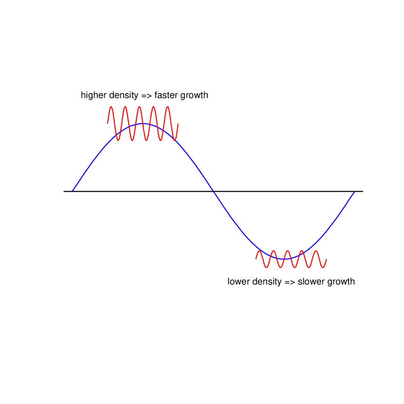
Figure 1: The fluctuating density field has both long and short wavelength modes. The short wavelength modes in an overdense region caused by a long wavelength mode effectively evolve as if they are in a universe with a higher mean density, hence they evolve faster. The oposite is true for short wavelength modes in an underdense region. This effect creates a correlation between the small scale power and the large scale density fluctuations.

In this paper we study the cross correlation statistic as applied to one dimensional data. Given a field $f(x)$ we compute

$$F(k) = \int dx\ e^{ikx}\ f(x)$$

$$F_{H}(k) = F(k)\ W_{k_{1}k_{2}}(k)$$ (1)

where $F_{H}(k)$ is a high-pass filtered field. Fields in real space are denoted with lower case letters, while their Fourier transforms are written with upper case letters. For example, in real space the high-passed filter field is denoted, $f_{H}(x)$. For simplicity we chose a simple high-pass window,

$$W_{k_{1}k_{2}}(k)=\left\{\begin{array}[]{ll}1&\mbox{if $k_{1}<k<k_{2}$}\\ 0&\mbox{otherwise,}\end{array}\right.$$ (2)

but the results are quite insensitive to this choice as long as the filter is non zero over a limited range of $k$ and the range is sufficiently wide. We are interested in how the power on small scales (the square of the amplitudes of the small scale modes) is distributed in space and whether this distribution is correlated with the low $k$ modes of $f$. For this purpose we transform the high passed filtered field $F_{H}$ to obtain $f_{H}(x)$. We define

$$f_{H}(x) = \int{dk\over 2\pi}F_{H}(k)e^{-ikx}$$

$$h(x) = f_{H}^{2}(x)$$

$$H(k) = \int dx\ e^{ikx}\ h(x).$$ (3)

The quantity $h(x)$ measures the amount of power in the wavelength band we chose, the square in its definition is introduced so that $h(x)$ indeed measures power and not just the amplitude of the small scale modes. Translational invariance ensures that if we had not introduced the square, the correlation between $h(x)$ and the long wavelength modes of $f(x)$ is zero. Since $h(x)$ is a field in real space it allows us to study how the small scale power depends on the position.

We may further introduce the auto and cross correlation power spectra of these quantities, as well as their cross correlation coefficient,

$$\mathop{\langle}F(k_{1})F(k_{1})\mathop{\rangle} = (2\pi)\delta^{D}(k_{1}+k_{2})P^{FF}(k_{1})$$

$$\mathop{\langle}H(k_{1})H(k_{1})\mathop{\rangle} = (2\pi)\delta^{D}(k_{1}+k_{2})P^{HH}(k_{1})$$

$$\mathop{\langle}F(k_{1})H(k_{1})\mathop{\rangle} = (2\pi)\delta^{D}(k_{1}+k_{2})P^{FH}(k_{1})$$

$$C(k) = {P^{FH}(k)\over\sqrt{P^{FF}(k)P^{HH}(k)}},$$ (4)

where $\mathop{\langle}\mathop{\rangle}$ denote ensemble average, $P^{FF}$ is the usual power spectrum of $f(x)$, $P^{HH}$ is the power spectrum of $h(x)$ and $P^{FH}$ is the cross correlation power spectrum between $f(x)$ and $h(x)$. By definition the cross correlation coefficient $C(k)$ we introduced is a number between $0$ and $1$, $C(k)=1$ means that in both fields modes of wavelength $k$ are always identical (or they always differ by the same multiplicative constant). We also want to emphasize that $h(x)$ depends quadratically on $f$ and thus $P^{FH}$ can be expressed as a three point function and $P^{HH}$ as a four point function of $f$. In general these depend on the shape and amplitude of primordial power spectrum, but for the cross-correlation coefficient $C(k)$ this dependence is weak and $C(k)$ is always close to unity (figure 2). In figure 2 we show the cross correlation coefficient for the one dimensional density field measured in a dark matter simulation. We used a PM simulation (Machacek and Bertschinger (1995)) of the standard CDM model (SCDM) model with $\sigma_{8}=0.6$. We use $16{\rm h^{-1}Mpc}$ box with $128^{3}$ particles. The three panels show the results for a different choice of the window $W_{k_{1}k_{2}}$, the range of which is shown using a horizontal line on the top of the figures. These ranges were chosen for later comparison with the Lyman-$\alpha$ forest data. We are only interested in the cross correlation between the small and large scales and for other wavevectors the cross correlation coefficient has been set to zero in the plots. We used 500 lines of sight chosen at random from one simulation box. The three power spectra were measured by averaging the results from all the lines of sight and the cross correlation coefficient was calculated by taking the ratios of the averaged quantities. Figure 2 shows that the correlation coefficient for the 1D density is very large, approximately $C\approx 0.8-0.85$ with only a mild dependence on scale. Other cosmological models predict very similar values for the cross-correlation coefficient.

Figure 2: The cross correlation coefficient is shown for the density field in one dimension as defined in the text. Each panel shows the result for a different choice of window $W_{k_{1}k_{2}}$. The range in wavevectors used ($k_{1}<k<k_{2}$) is shown by the horizontal line on the top of each panel. The cross correlation has been set to zero by hand for all wave-modes with $k>k_{1}$ or $k_{2}$, because we are not interested in those scales (see text for details).

3 Correlations between scales in the Lyman-$\alpha$ forest

.

In the last few years a very successful model of the Lyman $\alpha$ forest has been developed. This model, sometimes called fluctuating Gunn Peterson effect, attributes the absorption to the smoothly distributed gas mainly in low density regions. It has been shown that a very simple model in which the gas is assumed to trace the dark matter density and to be in ionization equilibrium with the ionizing background accurately describes the relevant physics. This model has been successfully used to compute the power spectrum of fluctuations of the flux and the probability distribution function of the flux (Croft et al. (1998, 1999)). We apply this model to PM simulations to predict what should be expected for the cross correlation, but we also compare it to hydrodynamical simulations (Bryan et al. (1999)).

In order to make predictions for this model we need to follow several steps which have been extensively discussed in the literature (eg. Croft et al. (1998)). The dark matter distribution is calculated with an N-body code, for which we use a PM algorithm (Machacek and Bertschinger (1995)). Pressure smooths the gas distribution relative to that of the dark matter and we apply a filter ($W_{F}(k)=e^{-k^{2}/k_{f}^{2}}$) to the dark matter density to mimic this effect. The smoothing scale $k_{f}$ is related to the Jeans scale and thus to the temperature of the gas, but also depends on the reionization history of the gas (Hui & Gnedin 1997a ). Thus although the order of magnitude of this length scale is known, we consider it a free parameter for the purpose of this paper (see also the method in Gnedin & Hui (1998)).

Once the simulation has been smoothed we construct simulated spectra by choosing random lines of sight in the simulation. We calculate the optical depth of a given fluid element as,

$$\tau=a_{0}(\rho/\bar{\rho})^{\beta}.$$ (5)

The constant $a_{0}$ can be related to physical parameters (eg. Croft et al. (1999); Hui et al. 1997b )

$$a_{0}=0.835\ ({1+z\over 4})^{6}\ ({\Omega_{b}h^{2}\over 0.02})^{2}\ ({T_{0}\over 10^{4}\ K})^{-0.7}\ ({h\over 0.65})^{-1}\ ({H(z)/H_{0}\over 4.46})^{-1}\ ({\Gamma\over 10^{-12}{\rm s}^{-1}})^{-1},$$ (6)

with $h=H_{0}/100{\rm kms^{-1}Mpc^{-1}}$, $\Omega_{b}$ baryon density in units of the critical density and $\Gamma$ is the photoionization rate. The position of each fluid element in velocity space is obtained by combining the Hubble flow and the peculiar velocity of the fluid element, $s=v_{pec}+H(z)x$, where $x$ and $s$ are the coordinates of the element in real and redshift space, respectively, and $v_{pec}$ is its peculiar velocity along the line of sight. We assume that the gas temperature is given by a simple equation of state (eg. Hui & Gnedin 1997a ),

$$T=T_{0}(\rho/\bar{\rho})^{\alpha},$$ (7)

where $\alpha$ and $\beta$ are related by $\beta=2-0.7\ \alpha$. Thermal broadening makes the optical depth produced by each fluid element to be distributed in velocity space as $\exp{-(\Delta s/b)^{2}}/b\sqrt{\pi}$, where $\Delta s$ is the displacement away from the position of the fluid element in velocity space and $b=(2kT/m_{p})^{1/2}\approx 13\ {\rm km\ sec^{-1}}(T/10^{4}{\rm K})$.

This model of the forest is a parametrized nonlinear transformation of the dark matter density to the flux $F=e^{-\tau}$ in velocity space along each line of sight. The parameters are not totally arbitrary, since they are related to physical quantities for which approximate values are known. The observation of the mean transmission can be used to fix one of the parameters, $a_{0}$. The mean transmission at redshift $z\sim 3$ is observed to be $\bar{F}=0.684\pm 0.023$ (McDonald et al. (1999)).

In the previous section we have shown that the one dimensional density field shows a very high correlation between the small scale power and the large scale density modes. The model we are considering for the observed flux in the Lyman-$\alpha$ forest is a complicated mapping from the dark matter density field. We investigate here the expected correlations for the observed flux. The dependence of the correlation coefficient on the choice of the smoothing scale is very weak (as long as the smoothing scale is taken to be independent of density). The reason for the small dependance on $k_{f}$ is that if the smoothing length is independant of density then it simply corresponds to multiplying the Fourier components of the density field by a fixed function of $k$. This fixed factor cancels when we take the ratio to compute the correlation coefficient. We use $k_{f}=40\ {\rm h\ Mpc}^{-1}$ throughout the paper, which is close to what is expected for reasonable reionization histories (Hui & Gnedin 1997a ). For each of the values of $T_{0}$ and $\alpha$ we explore, we set $a_{0}$ so that the generated spectra match the observed mean flux.

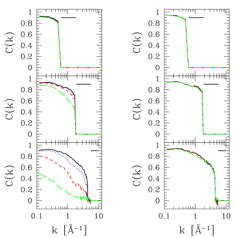
Figure 3: Cross correlation coefficient for the optical depth $\tau$ calculated as described in the text. The left (right) columns shows the results for $\alpha=0.6$ ($\alpha=0$). Different panels correspond to different choices of filter $W_{k_{1}k_{2}}$. There are four lines in each panel corresponding to different mean temperatures, $T_{0}=0.12,0.36,1.2,3.3\ \times 10^{4}K$ from top to bottom in the lowest left panel.

In figure 3 we show the measured cross correlation coefficient for the optical depth $\tau$ for different values of the temperature ($T_{0}=0.12,0.36,1.2,3.3\ \times 10^{4}K$) and several choices of the high pass filter. The left panels show the results for $\alpha=0.6$ while the right panels show $\alpha=0$, the isothermal equation of state. The temperatures we considered span the range allowed by other measurements (Schaye et al. (1999)). The cross correlation coefficient shown in the top panel is for the choice of the filter that preserves only the largest scales (smallest $k$) and is insensitive to the temperature regardless of $\alpha$. This is because these scales are larger than the thermal broadening scale and they do not depend on the amount of thermal smoothing.

When we study the smaller scale filters the results depend on $\alpha$. For $\alpha=0$ the results are independent of the temperature regardless of the scale. For $\alpha=0.6$ increasing the temperature reduces the cross correlation coefficient. When thermal broadening smooths the spectra with a filter independent of density ($\alpha=0$) the cross correlation is independent of temperature. Thermal broadening just alters the amplitude of the high $k$ modes, which cancels out when we compute the cross-correlation coefficient. Both the numerator and the denominator in the last line of equation (4) are changed by the same amount. This explains why for $\alpha=0$ the results show almost no change with $T_{0}$ (and also why the cross correlation is insensitive to $k_{f}$). For $\alpha>0$ the temperature depends on the density: denser regions are hotter and thermal broadening is more important there, suppressing the power on the smaller scales more than in colder regions. The higher the density, the higher the smoothing, the lower the small scale power. This effect is the opposite to what gravity does and thus decreases the cross correlation coefficient. To estimate the scale at which this should become important we note that the relation between $\AA$ and $\rm km/sec$ is such that

$$k[\AA]=61.67({4\over 1+z})k[{\rm km/s}]$$ (8)

A wavenumber in the last of our bands around $k\sim 7\mbox{\AA}^{-1}$ corresponds to $k^{-1}=10{\,\rm km/sec}$, which explains why temperatures above $T=(10{\,\rm km\ sec^{-1}})^{2}\sim 10^{4}K$ significantly reduce the cross correlation coefficient for the smallest scale filters when $\alpha\neq 0$.

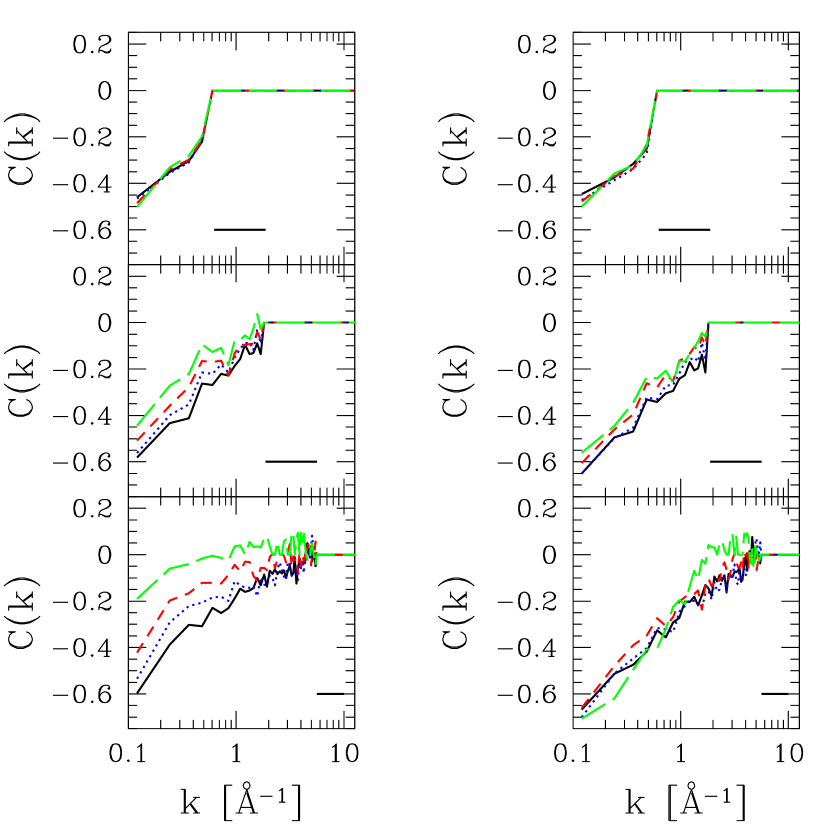
Figure 4: Cross correlation coefficient for the flux, using the same parameters as in figure 3.

In figure 4 we show the cross correlation coefficient for the flux, $F=e^{-\tau}$, which can be compared directly to the observations. The correlation coefficient is now negative because $e^{-\tau}$ is a decreasing function of $\tau$. It is also significantly lower, indicating that this nonlinear transformation suppresses some of the correlations. It would be interesting to explore the cross-correlation coefficient directly in the optical depth by performing the inverse of $F=e^{-\tau}$ on the data first, but for the purpose of this paper we will only use the data as observed, so we do not pursue this further. In the flux we also observe the effect of the thermal broadening as seen in the optical depth. Again for $\alpha=0.6$ the correlations decrease as we increase the temperature, and the effect is more important for the higher bands of $k$.

To test that our results on the cross correlation coefficient are not biased by using N-body simulations as opposed to hydrodynamic simulations we have measured $C(k)$ in the output of a hydrodynamic simulation for the same cosmological model described in Bryan et al. (1999). The results are very similar between the two outputs, specially on large scales ($k\,\mbox{${}^{<}_{\sim}$}\,1\AA^{-1}$). A detailed comparison will be presented elsewhere.

4 An application to QSO Q1422+231

In this section we present the results of the cross-correlation analysis applied to the Keck HIRES observed spectrum of Q1422+231 Kim et al. (1997). To measure the cross correlation we split the quasar spectrum between Ly$\alpha$ and Ly$\beta$ into ten separate pieces. Each piece has a length of 3200 km/sec (16 $h^{-1}{\rm Mpc}$), the same as our simulation. This facilitates the interpretation of the results and allows us to estimate the error bars using the variance between the ten subsamples. We are effectively considering each of the ten pieces as independent, which may not be a valid assumption, so we caution that the results presented here are preliminary. We will present a larger analysis elsewhere.

We measure $P^{FF}(k)$, $P^{HH}(k)$, $P^{HF}(k)$ in each of the ten sections of the quasar spectrum. The (normalized) power spectra are measured from the un-continuum-fitted data using the trend-removal technique as described in Hui et al. (2000). We choose 3 high passed windows as used in the simulations. We construct the cross correlation coefficient form the ratios of these power spectra for each of the 10 sections independently and estimate the variance from the fluctuations between the subsamples. Figure 5 shows the mean of the cross correlation in the 10 subsamples. The errorbars computed using the simulations agree with those inferred from the variance between the subsamples. It should be noted that because $C(k)$ is a number between -1 and 1, the shape of the error distribution is not Gaussian and the error bars in the plot should only be taken as an indication of the variance. For comparison we also show the values measured in the simulation for $\alpha=0$ and $T_{0}=1.2\ 10^{4}K$. The agreement between prediction and observations is quite striking, lending further support to the overall picture of the forest as being generated by gravitational instability.

To further check the agreement between the observed data and the simulations we computed the residuals from the mean of $C(k)$ for the different subsamples of the spectra. Figure 6 shows the histogram of these residuals, both for the data and simulations. The distribution of residuals is very similar for the two samples, so one can use the distribution observed in the simulations to constrain processes other than gravitational instability that could be affecting the observed cross correlations.

The first important conclusion to draw from figure 5 is that we observe a negative cross correlation coefficient in the range predicted by the simulations. Not only are the values of the cross correlation coefficient similar to those in our simulations but the distribution of their residuals from the mean is also very consistent. In the next section we use this measurement to constrain contamination from fluctuations in the continuum. Here we compare the smallest scale filter (the right panel in figure 5), in which we observe significant cross correlation, with the figure 4. The observed correlation argues against models with both high temperature $T_{0}$ and high $\alpha$ (the top lines in the bottom left panel of figure 4). More accurate constraints on these parameters from such observations will be presented elsewhere, as the details in this regime are somewhat sensitive to other parameters like the Jeans smoothing scale and numerical resolution. It seems however that this can be a promising way to study the state of the gas at high redshifts.

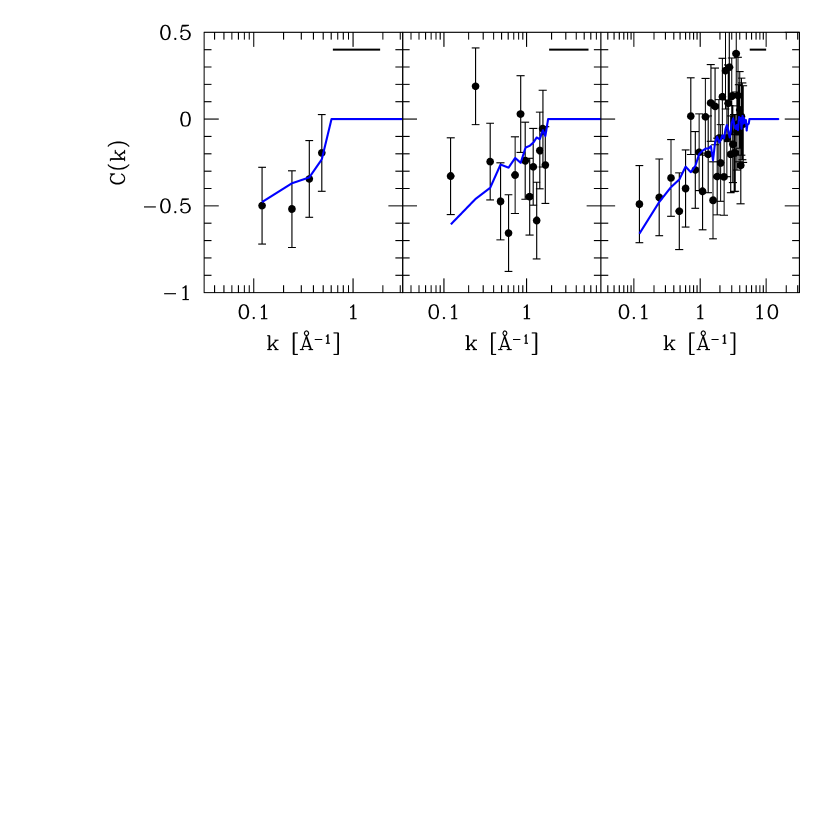
Figure 5: Cross correlation coefficient measured in Q1422+231 together with the prediction from simulation. The horizontal line on the top shows the range used to construct the high-passed filter. Each point represents the mean $C(k)$ averaged over the 10 subsamples of the quasar spectra. The error bars were computed from the simulations, but agree with the estimate from the variance between the subsamples.

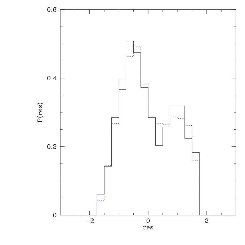
Figure 6: The distribution function of the residuals of the measured $C(k)$ for QSO1422+231 (dashed line) and simulations (solid line). The residuals are defined as $(C-\bar{C})/\sigma_{C}$ where $C$ is the cross correlation coefficient measured in each of the 10 subsamples of the spectra, $\bar{C}$ is the average over the subsamples and $\sigma_{C}^{2}=0.5*(\bar{C}^{2}+1)$ is a normalization factor introduced for convenience in the plotting.

5 Testing the continuum and the optical depth fluctuations

In previous sections we have calculated what we expect for the cross correlation coefficient in the flux of the Lyman $\alpha$ forest in the currently accepted model for the forest and compared that with the measurements in Q1422+231. This statistic can also be used as a test of the contamination from non-gravitationally induced fluctuations in the forest and in this section we want to explore its discriminatory power.

We consider the effects of the quasar continuum and optical depth fluctuations. We can model the observed flux as,

$$F(s)=[1+c(s)]e^{-\tau}$$ (9)

where $c$ is a slowly varying function of position across the spectrum. Continuum changes the overall level of the flux and so acts multiplicatively on the fluctuations produced by the neutral gas. This case also applies to any process that adds to the optical depth, such that $\tau\rightarrow\tau+\delta\tau$, if we identify $\delta\tau=\ln(1+c)$.

Let us consider the case where $c(s)$ has predominantly large scale power so that the fluctuations in $c$ dominate over the fluctuations in $e^{-\tau}$ on large scales. If we consider a region where $c(s)>0$ the flux will be larger than the mean flux in this region, $F(s)>\bar{F}$. On small scales, the power in this region will be enhanced because the continuum or optical depth fluctuations enter multiplicatively in the flux. The amplitude of all the small scale fluctuations is enhanced by a factor $[1+c(s)]$. Thus the continuum fluctuations induce a positive cross correlation between the large scales and the small scale power. This is opposite in sign of what gravity induces and constitutes the basis for the discriminatory power of this statistic.

The detailed predictions for the effect of the continuum will depend on its level of fluctuations compared to those induced by the absorption as a function of scale. For the purpose of the study here we assume that we can describe the continuum fluctuations with a power spectrum of shape similar to that of the Lyman $\alpha$ forest on large scales, but with an exponential cutoff at $k\sim 1$  Å ^-1. We will let the normalization of the additional power spectrum to be a free parameter which we try to constrain. We choose this shape for the power spectrum of fluctuations so that it is the most degenerate with the expected shape of the power spectrum induced by gravity, so that the presence of continuum fluctuations cannot be revealed by a change in the shape of the measured power spectrum. We introduced an exponential cutoff so that the fluctuations are only important on large scales, where we expect them to be the largest based on the continuum fluctuations on the red side of Ly-$\alpha$ (figure 7; see Hui et al. (2000)).

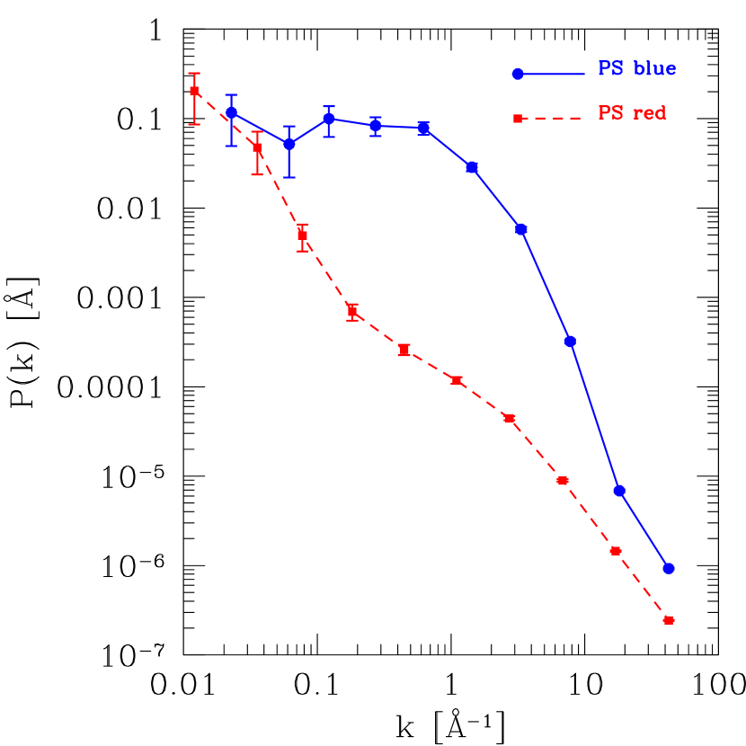
Figure 7: Power spectrum of the fluctuations in the flux on the red side and blue (L$\alpha$ forest) side of the L$\alpha$ line of of Q1422+231.

In figure 8 we show the expected cross-correlation for the lowest $k$ filter for several choices of the amplitude of the continuum power spectrum. As expected, increasing the amplitude drives the correlation to positive values. The effect of the fluctuations of the QSO continuum can be used to constrain the amplitude of the fluctuations using the measurements of Q1422+231. To do so we focus on the results in the lowest $k$ range. As we discussed in the previous section these are most insensitive to other parameters in our model and the predictions of our N-body model are in best agreement with the results of the full hydrodynamic simulations.

We can constrain the continuum fluctuations using a Monte Carlo technique. We generate random spectra with different levels of continuum contaminations to simulate the measurements of Q1422+231. We use realizations of Gaussian random field to simulate the continuum. We repeat this process many times and for several levels of contamination to measure the distribution of values for the cross correlation coefficient that we should observe in Q1422+231. We then compare these distributions with the measured values to put a constraint on the level of contamination. In figure 9 we show the distribution of measured cross-correlation coefficients in the simulations assuming that the continuum fluctuations are 10 %, 30 % and 40 % of the overall power of the flux fluctuations. We also show the distribution when there is no contamination. The upper panel is for $C(k=0.12)$, the lowest $k$ bin, and the bottom panel is for the average of the four bins. The vertical line on the x axis shows the measured value in Q1422+231. It is clear that continuum fluctuations that contribute 30 % of the measured power are ruled out and that even a 10 % contamination level is unlikely. This is in agreement with the expected level of continuum fluctuations based on the power spectrum of the red side of the Ly-$\alpha$ emission, which, except for the largest scales (not probed here), is significantly below the power spectrum of the blue side dominated by the Ly-$\alpha$ absorption (figure 7). With a larger sample of QSO it will be possible to explore also the scale dependence of the continuum contamination. Cross-correlation information can also be used to subtract out the contamination from the power spectrum, at least if it does not completely dominate the fluctuations on large scales as the results from figure 7 suggest.

We stress that as we discussed in the previous section we did not try to correct for continuum fluctuations before measuring the Fourier components of the flux. We directly measured the Fourier modes of the relative flux fluctuations in each chunk of the spectrum and did the same thing in our Montecarlo simulations. This is particularly important for our test because one can imagine that the continuum fitting procedure could introduce spurious correlations between scales that under some circumnstances could mimick the effect of gravity.

Figure 8: Cross correlation coefficient for different choices of the amplitude of the continuum fluctuations corresponding to 10, 30 and 40 % of the flux power spectrum. We also show the case of no contamination as a solid line.

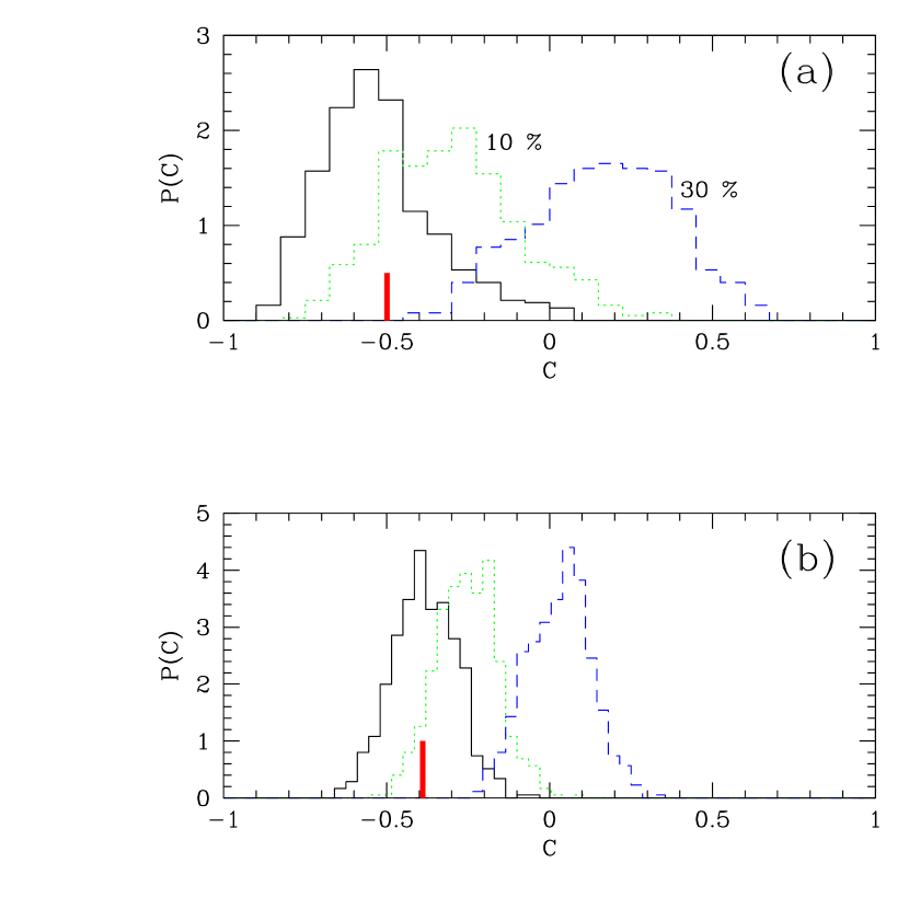
Figure 9: Histograms of cross correlation coefficients measured in simulations for cases when the size of continuum fluctuations is 10% and 30 % of the amplitude of the fluctuations in the flux. We also show the case of no continuum fluctuations (solid line). Panel (a) is for the lowest bin of our lowest high pass filter range, shown in the leftmost panel of figure 5) and panel (b) is for the average over all 4 bins for the same filter shown in the same panel. To construct the histogram we extracted 5000 lines of sight from the simulation, each line of sight has a length of $1/10$ of the spectra of Q1422+231. The vertical bar in each panel indicate the measurements from Q1422+231.

6 Conclusions

Gravity predicts that nonlinear evolution generates higher order correlations from an initially Gaussian density field. One of the consequences of the gravitational instability picture is that there should be a correlation between the power on small scales and the large scale modes of the density. This correlation is induced because in locally overdense regions the fluctuations grow faster, while the opposite is true for the underdense regions. While such a cross-correlation only uses a subset of all the information contained in the higher order correlations, it has the advantage of being relatively insensitive to the cosmological model and the initial spectrum of fluctuations. This allows one to separate the effects induced by gravity from those induced by other effects in a model independent way. We have presented a statistic that is sensitive to gravity and applied it to the flux measurements in the Lyman $\alpha$ forest.

The values of the correlation coefficient measured in Q1422+231 are in good agreement with what is found in the simulations. This is another confirmation of the overall picture of the forest based on the gravitational instability and ionization equilibrium. The agreement can also be used to constrain other processes that could contaminate large scale fluctuations in the forest and thus degrade the extraction of the dark matter power spectrum from them. If such processes unrelated to gravity were present they would suppress the cross-correlations. In this paper we estimate the level of fluctuations in the continuum of the quasar on large scales and show that even a 10% level of contamination on 10h^-1Mpc scales is unlikely, assuming the continuum has the same power spectrum shape as the fluctuations induced by gravity. With a larger sample of quasars we can expect to be able to determine the level of contamination as a function of scale, which will allow one to extract the dark matter power spectrum to significantly larger scales than current estimates permit (Croft et al. (1999); McDonald et al. (1999); see also Hui et al. (2000)).

The cross-correlation analysis can also be used to set constraints on the variation of other quantities, such as the parameters of the equation of state of the gas. The preliminary comparison of the cross correlation with the simulations seems to indicate that models with both high temperature and large $\alpha$ are inconsistent with the data. With a larger sample one should be able to determine with higher precision parameters such as the mean temperature of the gas and its equation of state. This will provide important constraints on the thermal history of the intergalactic medium at high redshifts.

The authors wish to thank Roman Scoccimarro and Greg Bryan for very helpful discussions. We also thank Greg Bryan for providing us with the results of his hydrodynamic simulations. We are grateful to Antoinette Songaila and Len Cowie for kindly making available the spectrum for Q1422+231. Support for this work is provided by the Hubble Fellowship (M.Z.) HF-01116-01-98A from STScI, operated by AURA, Inc. under NASA contract NAS5-26555, the NASA grant NAG5-8084 (U.S.), the NASA grant NAG5-7047, NSF grant PHY-9513835 and the Taplin Fellowship (L.H.).

References

- (1) Bernardeau F. 1994a, A&A, 291, 697
- (2) Bernardeau F. 1994b, ApJ, 433, 1
- Bi et al. (1992) Bi H. G., Boerner G., Chu Y.,1992, A&A, 266, 1
- Bi & Davidsen (1997) Bi H. G., Davidsen A. F. 1997, ApJ, 479, 523
- Bryan et al. (1999) Bryan G., Machacek M., Anninos P., Norman M. L. 1999, ApJ, 517, 13
- Cen et al. (1994) Cen R., Miralda-Escude J., Ostriker J. P., Rauch M. 1994, ApJ, 437, L9
- Croft et al. (1998) Croft R. A. C., Weinberg D. H., Katz N., Hernquist L. 1998, ApJ, 495, 44
- Croft et al. (1997) Croft R. A. C., Weinberg D. H., Hernquist L., Katz N. 1997, ApJ, 488, 532
- Croft et al. (1999) Croft R. A. C., Weinberg D. H., Pettini M., Hernquist L., Katz N. 1999, ApJ, 520, 1
- Frieman & Gaztañaga (1999) Frieman J. A., Gaztañaga E. 1999, ApJ, 521, L83
- Fry (1994) Fry J. N. 1994, Phys. Rev. Lett., 73, 215
- Fry et al. (1993) Fry J. N., Melott A. L., Shandarin S. F. 1993, ApJ, 412, 504
- Gaztañaga (1994) Gaztañaga E. 1994, MNRAS, 268, 913
- Gaztanaga & Croft et al. (1999) Gaztanaga E., Croft R. A. C. 1999 MNRAS309, 885
- Gneidn & Hui (1996) Gnedin N. Y., Hui L., 1996, ApJ, 472, 73
- Gnedin & Hui (1998) Gnedin N. Y., Hui L., 1998, MNRAS, 296, 44
- Goroff et al. (1986) Goroff M. H., Grinstein B., Rey S.-J., Wise M. B. 1986, ApJ, 311, 6
- Hernquist et al. (1995) Hernquist L., Katz N., Weinberg D. H., Miralda-Escude J. 1995, ApJ, 457, L5
- Hui et al. (2000) Hui L., Burles S., Seljak U., Rutledge R. E., Magnier E., Tytler D. 2000, submitted to ApJ, astro-ph 0005049
- (20) Hui L., Gnedin N. Y. 1997a, MNRAS, 292, 27
- (21) Hui L., Gnedin N. Y., Zhang Y. 1997b, ApJ, 486, 599
- Juszkiewicz et al. (1993) Juszkiewicz R., Bouchet F. R., Colombi S. 1993, ApJ, 412, L9
- Kim et al. (1997) Kim T. S., Hu E. M., Cowie L. L., Songaila, A. 1997, AJ, 114, 1
- McDonald et al. (1999) McDonald P., Miralda-Escude J., Rauch M., Sargent W. L. W., Barlow T. a. , Cen R., Ostriker J. P., preprint astro-ph/9911196
- Machacek and Bertschinger (1995) Machacek, M. and Bertschinger, E. 1995, American Astronomical Society Meeting, 186, 0207
- Miralda-Escude et al. (1996) Miralda-Escude J., Cen R., Ostriker J. P., Rauch M. 1996, ApJ, 471, 582
- Miralda-Escude et al. (2000) Miralda-Escude J., Haehnelt M., Rees M., 2000, ApJ, 530, 1
- Muecket et al. (1996) Muecket J. P., Petitjean P., Kates R. E., Riediger R. 1996, A&A, 308, 17
- Narayanan et al. (2000) Narayanan V. K., Spergel D. N., Dave R., Ma C. P. 2000, preprint astro-ph/0001247
- Reisenegger & Miralda-Escude (1995) Reisenegger A., Miralda-Escude J. 1995, ApJ, 449, 476
- Schaye et al. (1999) Schaye J., Theuns T., Leonard A., Efstathiou G. 1999, MNRAS, 310, 57
- Scoccimarro et al. (1998) Scoccimarro R., Colombi S., Fry J. N., Frieman J. A., Hivon E., Melott A. 1998, ApJ, 496, 586
- Scoccimarro et al. (1998) Scoccimarro R., Feldman H. A., Fry J. N., Frieman J. A. 2000, preprint astro-ph/0004087
- Theuns et al. (1998) Theuns T., Leonard A., Efstathiou G., Pearce F. R., Thomas P. A. 1998, MNRAS, 301, 478
- Wadsley & Bond (1996) Wadsley J. W., Bond J. R. 1996, Proceeding of the 12th Kingston Conference, eds. Clarke D., West M., PASP, astro-ph/9612148
- White & Croft (2000) White M., Croft R. A. C. 2000, preprint astro-ph/0001247
- Zhang et al. (1995) Zhang Y., Anninos P., Norman M. L. 1995, ApJ, 453, L57