HNCO in massive galactic dense cores

Abstract

We surveyed 81 dense molecular cores associated with regions of massive star formation and Sgr A in the $J_{\rm K_{-1}K{{}_{1}}}=5_{05}-4_{04}$ and $10_{010}-9_{09}$ lines of HNCO. Line emission was detected towards 57 objects. Selected subsamples were also observed in the $1_{01}-0_{00}$, $4_{04}-3_{03}$, $7_{07}-6_{06}$, $15_{015}-14_{014}$, $16_{016}-15_{015}$ and $21_{021}-20_{020}$ lines, covering a frequency range from 22 to 461 GHz. HNCO lines from the $K_{-1}=2,3$ ladders were detected in several sources. Towards Orion-KL, $K_{-1}=5$ transitions with upper state energies $E_{\rm u}/k\sim 1100$ and 1300 K could be observed.

Five HNCO cores were mapped. The sources remain spatially unresolved at 220 and 461 GHz ($10_{010}-9_{09}$ and $21_{010}-20_{020}$ transitions) with beam sizes of 24″ and 18″, respectively.

The detection of hyperfine structure in the $1_{01}-0_{00}$ transition is consistent with optically thin emission under conditions of Local Thermodynamic Equilibrium (LTE). This is corroborated by a rotational diagram analysis of Orion-KL that indicates optically thin line emission also for transitions between higher excited states. At the same time a tentative detection of interstellar HN¹³CO (the $10_{0,10}-9_{0,9}$ line at 220 GHz toward G 310.12-0.20) suggests optically thick emission from some rotational transitions.

Typical HNCO abundances relative to H₂ as derived from a population diagram analysis are $\sim 10^{-9}$. The rotational temperatures reach $\sim 500$ K. The gas densities in regions of HNCO $K_{-1}=0$ emission should be $n\ga 10^{6}$ cm^-3 and in regions of $K_{-1}>0$ emission about an order of magnitude higher even for radiative excitation.

HNCO abundances are found to be enhanced in high-velocity gas. HNCO integrated line intensities correlate well with those of thermal SiO emission. This indicates a spatial coexistence of the two species and may hint at a common production mechanism, presumably based on shock chemistry.

1 Introduction

Systematic studies of dense molecular cores in regions of high mass star formation (HMSF) are of great importance for our general understanding of star formation. In comparison with low mass star formation regions, so far only a few rather arbitrarily selected cores associated with HMSF have been investigated in some detail.

In recent years we performed extensive surveys of dense cores in regions of high mass star formation, mainly in CS (Zinchenko et al. 1995, 1998). We used water masers as signposts of high mass star formation. Both outer and inner Galaxy were covered by these surveys ($l\approx 120\degr-210\degr$ and $260\degr-308\degr$). The innermost part of the Galaxy ($l\approx 308\degr-360\degr$) was observed in a similar way by Juvela (1996). In addition, sources associated with water masers were surveyed in thermal SiO (Harju et al. (1998)) which is supposed to be a good indicator of shocks in molecular clouds. From these observations we derived basic physical parameters of the cores and constructed their statistical distributions (Zinchenko (1995), Zinchenko et al. (1998)). In order to investigate a range of core densities, observations of lines with different excitation conditions are needed. One of the interesting candidates is the HNCO (isocyanic acid) molecule.

HNCO was first detected by Snyder & Buhl (1972) in Sgr B2. Subsequent studies have concentrated mostly on the Galactic center region where the HNCO emission was found to be particularly strong (e.g., Churchwell et al. 1986, Wilson et al. 1996, Lindqvist et al. 1995, Kuan & Snyder 1996, Dahmen et al. 1997, Sato et al. 1997). A survey of HNCO emission throughout the Galaxy was made by Jackson et al. (1984) in the $J_{\rm K_{-1}K{{}_{1}}}=5_{05}-4_{04}$ and $4_{04}-3_{03}$ transitions with the 11 m NRAO telescope. Seven (from 18) clouds including Orion KL were detected at rather low levels of intensity (typically $\sim 0.2$ K on a $T_{\rm A}^{*}$ scale). Churchwell et al. (1986) obtained strict upper limits on HNCO $1_{01}-0_{00}$ and $2_{02}-1_{01}$ emission towards about 20 galactic sources with the 36.6 m Haystack antenna.

HNCO is a slightly asymmetric rotor. Its levels may be designated as $J_{\rm K_{-1}K_{1}}$ where $J$ is the total angular momentum and $K_{-1}$, $K_{1}$ are quantum numbers corresponding to the projection of $J$ on the symmetry axis for the limiting cases of prolate and oblate symmetric top, respectively (e.g. Townes & Schawlow 1975). The structure of the HNCO energy levels can be represented as a set of “ladders” with different $K_{-1}$ values, like for a symmetric top. However, due to the asymmetry of the molecule radiative transitions between different $K_{-1}$ ladders ($b$-type transitions) are allowed and, moreover, they are very fast. The corresponding component of the dipole moment is similar to its component for transitions inside the $K_{-1}$ ladders ($a$-type transitions). Churchwell et al. (1986) found that as a result the HNCO excitation is governed mostly by radiative rather than collisional processes (at least in Sgr B2).

On the basis of their estimates of source parameters Jackson et al. (1984) concluded that HNCO is a potentially valuable probe of the densest regions ($n\ga 10^{6}$ cm^-3) of molecular clouds. It was shown also that HNCO is rather sensitive to far infrared (FIR) radiation fields due to the fact that the lowest levels of the $K_{-1}=0,$ 1 and $K_{-1}=1,$ 2 ladders are separated by energies corresponding to FIR wavelengths (330 $\mu$m and 110 $\mu$m, respectively).

From this consideration it is clear that multitransitional data are needed to understand HNCO excitation and to derive the source properties. Bearing this in mind we undertook a survey of HNCO emission in various rotational lines, also trying to detect emission from higher excited $K-$ladders ($K_{-1}>0$). Five cores were mapped in HNCO to estimate the extent of the emission.

Several other species were observed simultaneously with HNCO. The most prominent are C¹⁸O and SO. In the following we thus also compare HNCO with C¹⁸O.

2 Observations

2.1 Source list

For this study we observed those dense cores showing particularly strong CS emission ($T_{\rm mb}>3$ K) in the surveys of Zinchenko et al. (1995, 1998) and Juvela (1996). Several strong SiO ($v=0$) sources detected by Harju et al. (1998) are also included in our sample. Sources observed at the SEST and at Onsala are presented in Tables 1, 2. Sources also observed at Effelsberg or at the HHT are marked in both tables.

We designate most sources according to their galactic coordinates. Exceptions are Orion KL and Sgr A. For Sgr A we use the position observed by Jackson et al. (1984) for comparison (known as the M-0.13-0.08 cloud, see Lindqvist et al. 1995). Common identifications with some well known objects are given in the last column.

Table 1: Source list for SEST observations.

Name	$\alpha(1950)$	$\delta(1950)$	Remarks
	(h) (m) (s)	(∘) (′) (′′)
G 261.64$-$2.09	08 30 23.2	$-$43 03 31
G 264.28$+$1.48	08 54 39.0	$-$42 53 30	RCW 34
G 265.14$+$1.45	08 57 36.3	$-$43 33 38	RCW 36
G 267.94$-$1.06	08 57 21.7	$-$47 19 04	RCW 38
G 268.42$-$0.85	09 00 12.1	$-$47 32 07
G 269.16$-$1.14	09 01 51.6	$-$48 16 43
G 270.26$+$0.83	09 14 58.0	$-$47 44 00	RCW 41
G 285.26$-$0.05	10 29 36.8	$-$57 46 40
G 286.20$+$0.17	10 36 34.8	$-$58 03 22
G 291.27$-$0.71	11 09 42.0	$-$61 01 55
G 291.57$-$0.43	11 12 54.0	$-$60 52 57	NGC 3603
G 294.97$-$1.73	11 36 51.6	$-$63 12 09
G 300.97$+$1.14	12 32 00.2	$-$61 23 44	RCW 65
G 301.12$-$0.20	12 32 31.3	$-$62 44 38
G 305.20$+$0.21	13 07 59.9	$-$62 18 50	RCW 74
G 305.36$+$0.21	13 09 21.2	$-$62 18 02
G 308.80$-$0.25	13 13 27.2	$-$62 42 56
G 308.00$+$2.02	13 29 24.3	$-$60 11 22
G 308.92$+$0.12	13 39 34.4	$-$61 53 45	RCW 79
G 309.92$+$0.48	13 47 12.5	$-$61 19 58
G 316.77$-$0.02	14 41 10.4	$-$59 35 30
G 316.81$-$0.06	14 41 36.4	$-$59 36 53
G 318.05$+$0.09	14 49 51.9	$-$58 56 40
G 323.74$-$0.25	15 27 49.8	$-$56 20 15
G 324.20$+$0.12	15 29 01.2	$-$55 46 12
G 326.47$+$0.70	15 39 28.2	$-$53 58 01
G 326.64$+$0.61	15 40 42.6	$-$53 56 29
G 328.30$+$0.43	15 50 15.3	$-$53 02 46
G 328.81$+$0.63	15 51 59.0	$-$52 34 24
G 328.24$-$0.54	15 54 04.9	$-$53 50 09
G 329.03$-$0.20	15 56 40.1	$-$53 04 08
G 330.95$-$0.19	16 06 03.4	$-$51 47 30
G 330.88$-$0.36	16 06 30.0	$-$51 58 14
G 331.28$-$0.18	16 07 36.0	$-$51 33 40
G 332.83$-$0.55	16 16 23.7	$-$50 45 45	RCW 106
G 333.13$-$0.43	16 17 12.6	$-$50 28 18
G 333.60$-$0.22	16 18 24.5	$-$49 59 08
G 337.40$-$0.40	16 35 08.1	$-$47 22 23
G 340.06$-$0.25	16 44 36.4	$-$45 16 26
G 345.01$+$1.80	16 53 18.8	$-$40 09 36
G 343.12$-$0.06	16 54 42.8	$-$42 47 49
G 345.51$+$0.35	17 00 53.6	$-$40 40 02
G 345.00$-$0.23	17 01 40.7	$-$41 25 07
G 345.41$-$0.94	17 06 02.3	$-$41 31 44
G 348.55$-$0.97	17 15 53.1	$-$39 00 57
G 350.10$+$0.09	17 16 01.0	$-$37 07 30
G 348.73$-$1.04	17 16 39.7	$-$38 54 17	RCW 122
G 351.41$+$0.64	17 17 32.5	$-$35 44 13
G 351.58$-$0.36	17 22 04.2	$-$36 10 11
G 351.78$-$0.54	17 23 20.9	$-$36 06 53
G 353.41$-$0.36	17 27 06.5	$-$34 39 41
G 359.97$-$0.46	17 44 10.4	$-$29 11 03
Orion KLa,b	05 32 47.0	$-$05 24 23
G 173.48$+$2.45c	05 35 51.3	35 44 16	S231
G 192.60$-$0.05b	06 09 58.2	18 00 17	S255
Sgr Aa	17 42 28.0	$-$29 04 01

^a also observed in Effelsberg, ^b also observed with HHT, ^c also observed in Onsala.

Table 2: Source list for Onsala observations.

Name	$\alpha(1950)$	$\delta(1950)$	Remarks
	(h) (m) (s)	(∘) (′) (′′)
G 121.30$+$0.66	00 33 53.3	63 12 32	RNO 1B
G 123.07$-$6.31	00 49 29.2	56 17 36	NGC 281
G 133.69$+$1.22	02 21 40.8	61 53 26	W3 (1)
G 133.95$+$1.07b	02 23 17.3	61 38 58	W3 (OH)
G 170.66$-$0.27	05 16 53.6	36 34 21	IRAS05168+3634
G 173.17$+$2.35	05 34 35.9	35 56 57	IRAS05345+3556
G 173.48$+$2.45b,c	05 35 51.3	35 44 16	S 231
G 173.72$+$2.70	05 37 31.8	35 40 18	S 235
G 188.95$+$0.89	06 05 53.7	21 39 09	S 247
G 34.26$+$0.15	18 50 46.4	01 11 10	IRAS18507+0110
G 40.50$+$2.54	18 53 47.0	07 49 26	S76 E
G 43.17$+$0.01a,b	19 07 49.8	09 01 17	W49 N
G 49.49$-$0.39a,b	19 21 26.2	14 24 44	W51 M
G 60.89$-$0.13	19 44 14.0	24 28 10	S87
G 61.48$+$0.10	19 44 42.0	25 05 30	S88B
G 70.29$+$1.60	19 59 50.0	33 24 17	K3-50
G 69.54$-$0.98b	20 08 09.9	31 22 42	ON1
G 77.47$+$1.77	20 18 50.0	39 28 45	JC20188+3928
G 75.78$+$0.34	20 19 51.8	37 17 01	ON2 N
G 81.87$+$0.78b	20 36 50.5	42 27 01	W75 N
G 81.72$+$0.57a,b	20 37 13.7	42 12 11	W75 (OH)
G 81.77$+$0.60	20 37 16.6	42 15 15	W75 S3
G 92.67$+$3.07	21 07 46.7	52 10 23	J21078+5211
G 99.98$+$4.17	21 39 10.3	58 02 29	IRAS21391+5802
G 108.76$-$0.95	22 56 38.4	58 31 04	JC22566+5830
G 108.76$-$0.98	22 56 45.2	58 29 10	S152(OH)
G 111.53$+$0.76a,b	23 11 36.1	61 10 30	S 158

^a also observed in Effelsberg, ^b also observed with HHT, ^c also observed with SEST.

2.2 Observational procedures

The most important parameters of our SEST-15m, OSO-20m, Effelsberg 100-m and HHT measurements are summarized in Tables 3, 4. Further details are given below for each instrument.

Table 3: Observing parameters ($\Delta\nu$ is the spectral resolution).

Molecule	Transitiona	Frequency	Telescope	Date	HPBW	$\eta_{\rm mb}$	$T_{\rm sys}^{b}$	$\Delta\nu$
		(MHz)			(″)		(K)	(kHz)
HNCO	$1_{01}-0_{00}$	21981.460	Eff. 100m	1998	40	0.3	50–100	12.5
	$4_{04}-3_{03}$	87925.252	OSO 20m	1997	40c	0.60c	210–290	250
	$5_{05}-4_{04}$	109905.758	OSO 20m	1997	35c	0.52c	300–450	250
	$5_{05}-4_{04}$	109905.758	SEST 15m	1997	47c	0.71c	200–270	86
	$7_{07}-6_{06}$	153865.080	SEST 15m	1997	33c	0.64c	150–180	86
	$10_{0,10}-9_{0,9}$	219798.320	SEST 15m	1997	24c	0.52c	190–360	86
	$15_{0,15}-14_{0,14}$	329664.535	HHT 10m	1999	25	0.50	900–6000	480
	$16_{0,15}-15_{0,14}$	351633.457	HHT 10m	1999	24	0.50	700–1000	480
	$21_{0,21}-20_{0,20}$	461450.670	HHT 10m	1999	18	0.38	900–2000	480
C18O	$1-0$	109782.160	OSO 20m	1997	35c	0.52c	300–450	1000
	$2-1$	219560.319	SEST 15m	1997	24c	0.52c	190–360	1400

^aThe frequencies and spectral resolutions for the observed $K_{-1}>0$ transitions are presented in Table 4.
^bThe system temperatures are given on a $T_{\rm A}^{*}$ scale.
^cBeam sizes and main beam efficiencies are obtained by interpolating the data from the SEST manual (for SEST) and those provided by L.E.B. Johansson (for OSO) at nearby frequencies.

Table 4: Frequencies and spectral resolutions for the observed $K_{-1}>0$ transitions. For other observing parameters see Table 3

Transition	Frequency	$\Delta\nu$
	(MHz)	(kHz)
$10_{2,9}-9_{2,8}$	219733.850	1400
$10_{2,8}-9_{2,7}$	219737.193	1400
$10_{3,8}-9_{3,7}$	219656.710	1400
$10_{3,7}-9_{3,6}$	219656.710	1400
$10_{4,7}-9_{4,6}$	219547.082	1400
$10_{4,6}-9_{4,5}$	219547.095	1400
$10_{5,6}-9_{5,5}$	219392.412	1400
$10_{5,5}-9_{5,4}$	219392.412	1400
$15_{2,14}-14_{2,13}$	329573.46	480
$15_{2,13}-14_{2,12}$	329585.09	480
$21_{2,20}-20_{2,19}$	461336.93	480
$21_{2,19}-20_{2,18}$	461368.88	480
$21_{3,18}-20_{3,17}$	461182.51	480
$21_{3,19}-20_{3,18}$	461182.45	480
$21_{4,17}-20_{4,16}$	460950.89	480
$21_{4,18}-20_{4,17}$	460950.89	480
$21_{5,16}-20_{5,15}$	460625.75	480
$21_{5,17}-20_{5,16}$	460625.75	480

2.2.1 SEST observations

The observations were performed with SIS receivers in a single-sideband (SSB) mode using dual beam switching with a beam throw of $\sim 12$′. At 220 GHz we used 2 acousto-optical spectrometers in parallel: (1) a 2000 channel high-resolution spectrometer (HRS) with 86 MHz bandwidth, 43 kHz channel separation and 80 kHz resolution and (2) a 1440 channel low-resolution spectrometer (LR1) with a 1000 MHz total bandwidth, 0.7 MHz channel separation and 1.4 MHz spectral resolution. The LR1 band was centered on the HNCO $10_{0,10}-9_{0,9}$ transition. However, it covered some other HNCO transitions too (see Table 4) as well as C¹⁸O (2–1), SO ($6_{5}-5_{4}$) and other lines (Fig. 1 shows a typical spectrum).

Figure 1: A SEST low resolution spectrum. For identified features, molecular species and transitions are given

The 110 and 154 GHz observations were performed simultaneously; the spectra were recorded by the HRS which band was split into two equal parts. The 220 GHz HRS spectra were smoothed to 170 kHz resolution and the 110 and 154 mm spectra were smoothed to 86 kHz resolution. Pointing was checked periodically by observations of nearby SiO masers; the pointing accuracy was $\la 5$″.

The standard chopper-wheel technique was used for the calibration. We express the results in units of main beam brightness temperature ($T_{\rm mb}$) assuming the main beam efficiencies ($\eta_{\rm mb}$) as given in Table 3. The temperature scale was checked by observations of Orion KL.

In most sources only one position was observed, corresponding typically to the peak of the CS emission. In addition, G 270.26+0.83 and G 301.12$-$0.20 were mapped with a spacing of 10″.

2.2.2 Onsala observations

At Onsala, the 110 GHz observing procedure was very similar to that at the SEST. The observations were also performed in a dual beam switching mode with a beam throw of 11$\aas@@fstack{\prime}$5. The front-end was a SIS receiver tuned to SSB operation. As backend we used 2 filter spectrometers in parallel: a 256 channel filterbank with 250 kHz resolution and a 512 channel filterbank with 1 MHz resolution. The calibration procedure was the same as at the SEST. The pointing accuracy checked by observations of nearby SiO masers was $\la 5$″. The strongest HNCO source from the Onsala sample, W51M, was mapped with 40″ spacing.

2.2.3 Effelsberg observations

The 22 GHz observations in Effelsberg were performed with a K-band maser amplifier using position switching. The offset positions were displaced by 10′–15′ symmetrically in azimuth. Pointing was checked periodically by observations of nearby continuum sources; the pointing accuracy was $\la 10$″. The integration time per position was a few hours.

The main beam temperature scale was checked by observations of nearby continuum calibration sources, NGC 7027 and W3(OH); for Sgr A we used Sgr B2. The fluxes for the first two sources were taken from Ott et al. (1994). The Sgr B2 flux at 1.3 cm was taken from Martín-Pintado et al. (1990).

2.2.4 HHT observations

To observe the HNCO $J$ = 21–20 lines at 461 GHz we have used the Heinrich Hertz Telescope (HHT) on Mt. Graham (Baars & Martin 1996) during Feb. 1999 with a beamwidth of 18^′′. Spectra were taken employing an SIS receiver with backends consisting of two acousto optical spectrometers with 2048 channels each, channel spacing $\sim$480 and $\sim$120 kHz, frequency resolution $\sim$930 and 230 kHz, and total bandwidths of $\sim$1 GHz and 250 MHz, respectively. Receiver temperatures were $\sim$150 K, system temperatures were $\sim$1000 K on a $T_{\rm A}^{*}$ scale. The receiver was sensitive to both sidebands. Any imbalance in the gains of the lower and upper sideband would thus lead to calibration errors. To account for this, we have observed the CO $J$ = 4–3 line of Orion-KL with the same receiver tuning setup and obtain $T_{\rm A}^{*}$ $\sim$ 70 K, in good agreement with Schulz et al. (1995).

HNCO $J=16-15$ (351.63346 GHz) and $J=15-14$ (329.66454 GHz) line emission was observed with a dual channel SIS receiver in early April 1999 at the HHT. The beamwidth was 22″, receiver temperatures were 135 K; system temperatures were $\sim$700 K on a $T_{\rm A}^{*}$ scale. The receivers were also sensitive to both sidebands. We have used published spectra from Orion-KL and IRC+10216 as calibrators (Groesbeck et al. (1994); Schilke et al. (1997)).

All results displayed are given in units of main beam brightness temperature ($T_{\rm mb}$). This is related to $T_{\rm A}^{*}$ via $T_{\rm mb}$ = $T_{\rm A}^{*}$ ($F_{\rm eff}$/$B_{\rm eff}$) (cf. Downes 1989). The main beam efficiency, $B_{\rm eff}$, was 0.38 at 461 GHz and 0.5 at 330 and 352 GHz as obtained by measurements of Saturn. The forward hemisphere efficiency, $F_{\rm eff}$, is 0.75 at 461 GHz and 0.9 at 330 and 352 GHz (D. Muders, priv. comm.). The HHT is with an rms surface deviation of $\sim$20$\mu$m (i.e. $\lambda$/30 at 461 GHz) quite accurate. Thus emission from the sidelobes should not be a problem.

Pointing was obtained toward Jupiter (continuum pointing) and toward Orion-KL and R Cas (line pointing) with maximum deviations of order 5^′′. Observations were carried out in a position switching mode with the off-position $\sim$1000^′′ offset from the source position.

2.3 Data reduction and analysis

We have reduced the data and produced maps using the GAG (Groupe d’Astrophysique de Grenoble) software package. The measured spectra were fitted by one or more gaussian components.

3 Results

3.1 One-point observations

HNCO was detected in 36 SEST sources (from 56 observed) and in 22 OSO sources (from 27). Because of one source belonging to both samples, the total number of detected objects is 57. In many cases $K_{-1}>0$ transitions were detected too. The gaussian line parameters are presented in Tables 5–14 (Tables 7–14 are available only electronically). It is worth noting that a single-gaussian fit is clearly insufficient in many cases because the lines have broad wings and other non-gaussian features. Therefore, the values in the tables give only a rough representation of the line profiles (the integrated intensities were obtained by integrating over the lines in most cases).

Table 5 summarizes the 220 GHz SEST results for HNCO $10_{0,10}-9_{0,9}$ and C¹⁸O. The Onsala $5_{05}-4_{04}$ and C¹⁸O results are presented in Table 6. The 220 GHz results for the $K_{-1}=2$, 3 ladders are given in Tables 7, 8. The 110 and 154 GHz SEST data are displayed in Table 9. The Onsala 88 GHz data are summarized in Table 10. The Effelsberg data are presented in Table 11. Tables 12–14 contain the HHT data. We fitted the Effelsberg spectra with 3-component gaussians with fixed separations corresponding to the hyperfine structure of the $1_{01}-0_{00}$ transition.

Table 5: C¹⁸O ($2-1$) and HNCO ($10_{0,10}-9_{0,9}$) integrated intensities and gaussian line parameters at the indicated positions (cf. Tables 1,2) measured at SEST. The numbers in the brackets are the statistical uncertainties in the last digits (standard deviations).

			C18O ($2-1$)					HNCO ($10_{0,10}-9_{0,9}$)
Source	$\Delta\alpha$	$\Delta\delta$	$\int T_{\rm mb}dv$	$T_{\rm mb}$	$V_{\rm LSR}$	$\Delta V$		$\int T_{\rm mb}dv$	$T_{\rm mb}$	$V_{\rm LSR}$	$\Delta V$
	(″)	(″)	(K$\cdot$km/s)	(K)	(km/s)	(km/s)		(K$\cdot$km/s)	(K)	(km/s)	(km/s)
G 261.64	20	0	17.22(05)	3.73(01)	13.76(01)	4.02(02)		0.63(05)	0.15(01)	13.69(16)	3.87(39)
G 264.28	0	–40	3.41(04)	0.90(01)	5.39(02)	3.36(05)		0.17(03)	0.07(01)	6.12(25)	2.32(46)
G 265.14	–40	0	19.16(06)	4.63(02)	6.75(01)	3.68(02)
G 267.94	0	0	14.08(07)	2.59(01)	1.04(01)	4.68(03)
G 268.42	0	0	29.38(06)	5.57(01)	2.55(00)	4.60(01)		0.28(05)	0.07(01)	3.01(36)	3.92(73)
G 269.16	0	40	24.95(08)	4.30(02)	9.72(00)	5.09(02)		0.79(07)	0.18(02)	9.64(18)	4.05(44)
G 270.26	–20	20	16.28(05)	3.24(01)	8.67(01)	4.55(02)		1.07(06)	0.24(02)	9.92(12)	4.25(30)
G 285.26	0	0	10.16(06)	1.76(01)	2.47(01)	5.11(04)		0.50(09)	0.07(01)	1.64(65)	7.06(156)
G 286.20	40	–40	14.53(04)	3.14(01)	–20.86(01)	4.14(01)
G 291.27	–40	–40	28.39(06)	5.21(01)	–23.95(01)	4.93(01)		0.56(07)	0.12(02)	–23.80(25)	4.25(79)
G 291.57	0	0	7.59(07)	1.13(01)	13.12(03)	6.03(07)
G 294.97	0	0	15.77(05)	4.02(02)	–9.24(01)	3.31(01)
G 300.97	0	40	23.13(05)	4.39(01)	–43.89(01)	4.64(01)
G 301.12	80	–80	44.35(18)	7.13(03)	–40.01(01)	5.44(03)		4.15(08)	0.61(01)	–39.37(06)	6.43(16)
G 305.20	0	0	22.98(07)	3.41(01)	–42.13(01)	6.39(02)		1.84(10)	0.17(01)	–40.73(26)	10.12(71)
G 305.36	0	0	28.45(08)	4.47(01)	–36.60(01)	5.78(02)
G 308.00	0	0	13.38(05)	3.01(01)	–23.22(01)	3.85(02)		0.42(06)	0.14(02)	–21.63(16)	2.42(35)
G 308.80	0	0	16.54(07)	2.73(01)	–33.11(01)	5.27(03)		1.12(09)	0.15(01)	–32.57(29)	7.13(62)
G 308.92	0	0	25.96(07)	5.07(02)	–51.46(01)	4.55(02)		0.18(04)	0.10(03)	–51.08(18)	1.66(43)
G 309.92	0	0	22.08(07)	4.32(02)	–57.60(01)	4.35(02)
G 316.77	20	20	15.30(08)	2.51(01)	–41.05(01)	5.48(04)
G 316.81	0	20	17.51(08)	2.85(01)	–39.82(01)	5.63(03)
G 318.05	0	0	27.62(07)	5.63(02)	–50.48(01)	4.31(02)
G 323.74	0	20	4.42(06)	1.11(02)	–50.46(02)	3.29(06)
G 324.20	0	30	17.16(09)	2.39(02)	–89.27(02)	6.11(04)
G 326.47	0	0	12.13(09)	2.18(02)	–42.61(02)	4.59(05)		1.41(13)	0.16(02)	–41.39(35)	8.17(99)
G 326.64	0	0	35.04(08)	7.97(02)	–40.24(00)	3.95(01)		0.46(08)	0.10(01)	–39.24(40)	4.31(71)
G 328.24	0	0	24.60(09)	3.21(01)	–43.69(01)	7.11(03)
G 328.30	0	0	25.83(10)	3.56(02)	–92.92(01)	6.47(03)
G 328.81	0	0	55.86(15)	8.60(03)	–42.67(01)	5.34(02)		4.65(10)	0.60(02)	–41.37(07)	6.37(20)
G 329.03	0	0	13.89(08)	2.11(01)	–44.19(02)	5.57(04)		1.71(09)	0.28(02)	–43.70(15)	5.69(41)
G 330.88	0	0	43.65(23)	6.92(04)	–63.38(01)	5.45(04)		2.59(14)	0.34(02)	–62.78(18)	7.08(45)
G 330.95	20	20	59.42(16)	6.79(02)	–92.16(01)	8.36(03)		2.83(12)	0.27(01)	–91.38(21)	9.77(44)
G 331.28	40	–20	21.07(09)	3.86(02)	–89.39(01)	5.01(03)
G 332.83	0	–20	85.39(13)	10.90(02)	–57.94(01)	7.13(01)		3.24(13)	0.44(02)	–57.38(14)	6.92(33)
G 333.13	0	0	59.60(17)	8.28(03)	–52.55(01)	6.13(02)		1.07(13)	0.12(02)	–52.22(38)	6.89(140)
G 333.60	20	0	40.04(14)	4.10(02)	–49.60(02)	8.78(04)
G 337.40	20	20	43.56(10)	7.48(02)	–41.77(01)	5.29(01)		2.81(16)	0.37(03)	–40.69(16)	6.42(49)
G 340.06	0	0	34.59(13)	4.60(02)	–54.62(01)	6.59(03)		1.25(13)	0.17(02)	–53.55(37)	6.97(81)
G 343.12	0	0	16.80(17)	2.84(03)	–31.08(03)	5.24(07)		0.59(11)	0.13(02)	–31.12(43)	4.34(87)
G 345.00	0	0	27.05(40)	2.74(06)	–27.58(07)	7.12(16)		3.56(13)	0.39(02)	–26.85(15)	8.51(38)
G 345.01	0	0	44.61(08)	6.99(01)	–15.04(01)	5.79(01)		1.39(10)	0.25(02)	–14.27(18)	5.28(47)
G 345.41	0	0	36.99(09)	6.46(02)	–22.11(01)	5.17(02)
G 345.51	0	0	32.29(13)	5.03(03)	–18.45(01)	5.31(03)		1.10(12)	0.22(03)	–17.34(25)	4.70(60)
G 348.55	0	0	31.34(12)	4.32(02)	–16.16(01)	6.36(03)
G 348.73	0	0	76.64(12)	11.80(02)	–12.68(00)	5.78(01)		1.38(09)	0.25(02)	–11.16(17)	5.12(38)
G 350.10	0	0	27.58(11)	2.61(01)	–68.83(02)	9.98(04)		0.87(14)	0.07(01)	–68.18(99)	11.77(160)
G 351.41	0	0	57.97(20)	9.05(04)	–7.51(01)	5.57(03)		3.68(20)	0.42(03)	–7.60(18)	7.45(62)
G 351.58	0	0	24.04(12)	3.34(02)	–96.43(00)	6.37(04)		2.20(10)	0.36(02)	–94.72(13)	5.67(31)
G 351.78	0	0	88.86(38)	10.40(06)	–3.55(02)	6.11(04)		10.54(15)	1.08(02)	–2.95(05)	8.59(14)
G 353.41	0	0	55.52(10)	8.52(02)	–16.35(01)	6.05(01)		1.30(12)	0.25(02)	–16.11(22)	4.92(52)
G 359.97	0	0	20.16(09)	5.28(02)	17.71(01)	3.57(02)
Orion KL	0	0	53.52(135)	5.16(23)	7.69(11)	6.99(35)		52.50(70)	3.90(08)	7.16(07)	10.38(23)
Sgr A	0	0	31.22(48)	1.50(03)	11.96(15)	17.51(37)		12.95(25)	1.07(02)	14.19(10)	10.96(26)
S 231	0	0	8.10(09)	1.55(02)	–17.10(03)	4.71(07)		0.36(08)	0.15(03)	–15.45(26)	2.25(55)
S 255	0	0	15.50(06)	3.50(02)	6.67(01)	3.97(02)		0.53(07)	0.15(02)	8.24(23)	3.26(47)

Table 6: C¹⁸O ($1-0$) and HNCO ($5_{05}-4_{04}$) integrated intensities and gaussian line parameters at the indicated positions (cf. Tables 1,2) measured at Onsala. The numbers in the brackets are the statistical uncertainties in the last digits (standard deviations).

			C18O ($1-0$)					HNCO ($5_{05}-4_{04}$)
Source	$\Delta\alpha$	$\Delta\delta$	$\int T_{\rm mb}dv$	$T_{\rm mb}$	$V_{\rm LSR}$	$\Delta V$		$\int T_{\rm mb}dv$	$T_{\rm mb}$	$V_{\rm LSR}$	$\Delta V$
	(″)	(″)	(K$\cdot$km/s)	(K)	(km/s)	(km/s)		(K$\cdot$km/s)	(K)	(km/s)	(km/s)
G 121.30	0	0	5.94(18)	1.30(07)	–17.32(09)	3.55(22)		0.98(14)	0.40(06)	–17.57(16)	2.30(37)
G 123.07	0	0	3.19(14)	0.78(06)	–30.28(08)	3.81(32)		1.07(20)	0.12(02)	–31.14(84)	8.21(182)
G 133.69	0	–40	8.39(20)	1.22(03)	–42.38(08)	5.94(19)		0.55(14)	0.14(03)	–43.37(51)	3.77(106)
G 133.95	0	0	10.07(19)	1.71(04)	–47.60(05)	5.12(13)		1.38(24)	0.13(03)	–46.75(77)	9.95(231)
G 170.66	0	0	2.19(20)	0.56(05)	–15.27(24)	3.37(35)
G 173.17	0	0	4.50(27)	0.87(07)	–19.83(13)	4.78(40)
G 173.48	0	0	3.85(19)	0.76(04)	–16.22(12)	4.77(28)		1.25(20)	0.33(08)	–15.98(20)	2.68(69)
G 173.72	0	0	3.32(20)	0.97(09)	–16.83(12)	3.64(38)		0.49(14)	0.21(06)	–17.58(32)	2.22(72)
G 188.95	0	0	3.40(33)	0.70(09)	2.93(20)	4.54(66)
G 34.26	0	0	31.00(28)	4.45(04)	57.80(03)	6.47(07)		2.89(20)	0.54(04)	30.73(18)	5.55(41)
G 40.50	0	0	4.69(13)	0.81(03)	32.61(07)	5.22(20)		0.60(20)	0.14(08)	32.54(47)	3.94(237)
G 43.17	0	0	25.71(40)	1.45(02)	7.91(13)	14.84(28)		3.31(28)	0.24(02)	8.77(56)	12.97(118)
G 49.49	0	0	48.02(50)	2.99(04)	57.82(08)	12.45(19)		7.93(30)	0.69(03)	56.77(19)	10.20(50)
G 60.89	0	0	6.17(24)	1.33(07)	22.40(07)	4.35(26)		0.91(25)	0.14(03)	21.15(94)	7.07(143)
G 61.48	0	0	4.65(19)	1.12(06)	21.85(09)	3.82(23)
G 69.54	0	0	9.26(21)	1.98(05)	11.19(04)	4.52(14)		2.80(22)	0.43(04)	11.04(20)	5.38(57)
G 70.29	0	0	6.06(16)	0.70(02)	–24.28(10)	7.60(25)
G 75.78	0	0	8.96(18)	1.43(04)	–0.04(06)	5.28(14)		1.58(22)	0.16(02)	–1.88(66)	9.28(145)
G 77.47	0	0	5.59(16)	1.16(03)	0.50(07)	3.98(13)		1.00(20)	0.14(03)	0.98(72)	6.75(151)
G 81.72	0	0	19.07(22)	3.74(04)	–2.77(03)	4.49(06)		3.20(20)	0.53(04)	–2.71(19)	5.55(41)
G 81.77	0	0	8.23(13)	1.97(05)	–4.16(04)	3.65(11)		1.12(12)	0.25(04)	–3.97(19)	3.71(57)
G 81.87	0	0	13.45(24)	2.44(05)	9.36(05)	4.73(10)		2.37(28)	0.36(06)	9.52(31)	5.61(106)
G 92.67	0	0	4.22(16)	1.12(03)	–6.12(08)	3.66(12)		0.82(14)	0.21(04)	–5.26(37)	3.68(70)
G 99.98	0	0	5.21(14)	1.33(04)	0.67(06)	3.64(11)		0.46(10)	0.23(07)	0.67(15)	1.21(39)
G 108.76–0.95	0	0	6.79(16)	1.69(08)	–50.78(04)	3.77(20)		0.63(12)	0.23(06)	–50.63(22)	2.00(54)
G 108.76–0.98	0	0	11.97(17)	3.09(05)	–51.13(04)	3.51(06)		0.67(16)	0.16(04)	–51.08(45)	4.01(110)
G 111.53	0	0	12.22(22)	1.80(04)	–56.23(05)	6.18(14)		2.74(20)	0.55(05)	–56.44(16)	4.66(42)

Examples of measured spectra are given in Figs. 2, 3. Fig. 2 shows spectra of a few sources covering $K_{-1}=0$, 2 and 3 transitions at 220 GHz. Fig. 3 presents HNCO spectra in the HNCO $K_{-1}=0$ transitions at different wavelengths for several sources.

Figure 2: Examples of 220 GHz HNCO spectra obtained at SEST covering $K_{-1}=0$, 2 and 3 transitions

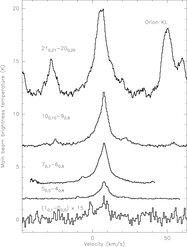
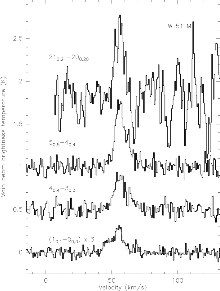
Figure 3: HNCO $K_{-1}=0$ lines in four selected sources. For the $1_{01}-0_{00}$ transition a 3-component gaussian (according for hyperfine structure) is superposed

The HNCO line profile in Orion KL can be decomposed into at least two components which likely correspond to the so-called classical “Hot Core” and “Plateau” outflow components (see, e.g., Harris et al. 1995). The ratio between these components is practically the same for the $5_{05}-4_{04}$, $7_{07}-6_{06}$ and $10_{0,10}-9_{0,9}$ lines: $\sim 60$% of the emission originates from the “Plateau” outflow source. The other lines do not allow such decomposition due to their weakness or blending with other spectral features.

An inspection of Table 5 shows that the derived C¹⁸O velocities are systematically lower (more negative) than the HNCO ones. The difference is $\sim-1$ km/s on the average. This can be an instrumental effect: the C¹⁸O line was located far away from the center of the spectrometer band and a possible non-linearity in the frequency response could lead to the apparent displacement of the line on the velocity axis. This remark is applicable also for the higher $K_{-1}$ HNCO lines.

3.2 Maps

In order to estimate source sizes and their spatial association with YSO and infrared (IR) sources we mapped 2 southern sources in the $10_{0,10}-9_{0,9}$ HNCO line and Orion KL, W49N and W51M in the $15_{0,15}-14_{0,14}$, $16_{0,16}-15_{0,15}$ and $21_{0,21}-20_{0,20}$ lines. W51M was mapped also in the $5_{05}-4_{04}$ line. Three of these maps are presented in Fig. 4.

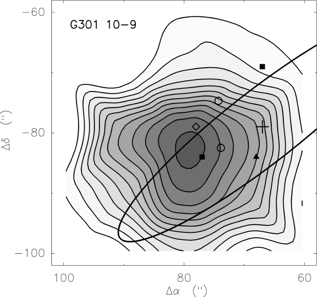
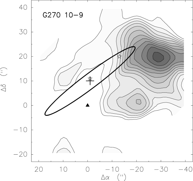
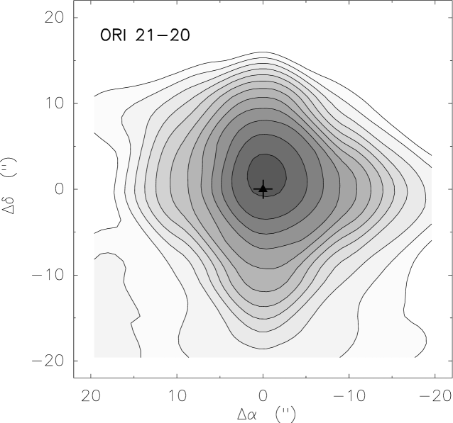
Figure 4: The HNCO $10_{0,10}-9_{0,9}$ integrated intensity maps of G301.12–0.20 and G270.26+0.83 and HNCO $21_{0,21}-20_{0,20}$ integrated intensity map of Orion KL. The levels start from 15% of the peak intensities in steps of 7.5%. The peak intensities equal to 4.4, 1.5 and 95.0 K$\cdot$km s^-1 for G301.12–0.20, G270.26+0.83 and Orion KL, respectively. The beam widths are 24″ for the first two objects and 18″ for Orion KL. For the first two objects the large crosses indicate IRAS positions, small stars show NIR sources, triangles mark H₂O masers, squares correspond to OH masers and diamonds show methanol masers (for references see Lapinov et al. 1998). Open circles mark UC H ii regions (Walsh et al. 1998). The IRAS uncertainty ellipses are shown. For Orion KL only the IRc 2 position is indicated

The sources remain spatially unresolved. E.g. for G 301.12–0.20 we obtain a FWHM $\approx 29$″ in right ascension (from the strip scan across the map) which is very close to the beam size at this frequency (24″).

3.3 Detection of the $K_{-1}=5$ HNCO transition

The highest $K_{-1}$ HNCO transition reported so far was $K_{-1}=4$ (the $10_{4}-9_{4}$ line) in Orion (Sutton et al. 1985). This line is located on the shoulder of the strong C¹⁸O $J=2-1$ line. In Fig. 5 we show parts of our Orion 220 GHz low resolution spectrum and 461 GHz spectra with $K_{-1}=2$, 3, 4 and even 5 features (the $K_{-1}=1$ transition is outside our band). The rest frequencies are assumed to be equal to those given in the JPL catalogue for the strongest components of the corresponding transitions (for $K_{-1}=2$ at 220 GHz we took the mean of the frequencies of the two strongest components).

Figure 5: Left panel: parts of the Orion low-resolution 220 GHz spectrum corresponding to higher $K_{-1}$ HNCO transitions. The profiles are aligned in velocity. No baselines are subtracted but the subspectra are shifted along the $y$-axis for clarity. The dashed vertical line corresponds to $V_{\rm LSR}=6.5$ km s^-1. Right panel: the same for the 461 GHz spectrum. Here the dashed vertical line corresponds to $V_{\rm LSR}=7.5$ km s^-1

There is a weak bump in the redshifted C¹⁸O $J=2-1$ wing which can be attributed to HNCO $10_{4}-9_{4}$. Due to the uncertainty in fitting the C¹⁸O line profile the intensity of the HNCO feature cannot be reliably determined but it is lower than reported by Sutton et al. (1985). Our best estimate for the integrated intensity is $\int T_{\rm mb}dv\sim 0.7$ K km/s, but a reliable error cannot be given.

There is also a feature at the $K_{-1}=5$ frequency in the 220 GHz spectrum. It is located in the wing of a C₂H₃CN line. The integrated intensity is $\int T_{\rm mb}dv=0.27\pm 0.06$ K km/s. The identification of this feature with HNCO seems to be reliable. The only other candidate is the C₂H₅OH $14_{21,2}-13_{11,2}$ line at 219391.81 MHz. However, there is no sign of other ethanol lines in our spectrum so we reject this alternative. In the 461 GHz spectrum the $K_{-1}=5$ feature is clearly detected. Its integrated intensity is $\int T_{\rm mb}dv=1.4\pm 0.2$ K km/s.

3.4 Hyperfine splitting, HN¹³CO and optical depths

The HNCO lines are split into several hyperfine components mainly due to the ¹⁴N spin. This splitting is clearly seen in the $1_{01}-0_{00}$ transition (Fig. 3) at 22 GHz. Earlier HNCO hyperfine structure in the $1_{01}-0_{00}$ line was only observed in the dark cloud TMC-1 (Brown (1981)) where possible deviations from the optically thin LTE (Local Thermodynamic Equilibrium) intensity ratios (3:5:1) were found. In our spectra the hyperfine ratios are consistent with the optically thin LTE values. Taking into account the measurement uncertainties, an upper limit on the optical depth in this transition for the sources detected in Effelsberg is $\tau\la 1$.

To the best of our knowledge no isotopomer of HNCO except the main one has been detected in space yet. This detection would be important for estimates of HNCO optical depths which are believed to be small (e.g. Jackson et al. 1984, Churchwell et al. 1986). The frequency separations between the HN¹³CO and the main isotopomer lines are rather small corresponding to a few km/s, so in sources with broad lines like Orion A or Sgr A the HN¹³CO lines will be blended. However, there are some strong HNCO sources in our sample with narrower lines which show features attributable to HN¹³CO. The most reliable one is seen in the G 301.12–0.20 $10_{0,10}-9_{0,9}$ spectrum (Fig. 6). A weak feature on the blue shoulder of the main isotope line is very close in frequency to the expected location of the HN¹³CO line .

Figure 6: The HNCO $10_{0,10}-9_{0,9}$ line in G301.12–0.20 in comparison with the C³⁴S(2–1) line. The expected location of the HN¹³CO $10_{0,10}-9_{0,9}$ line is shown

For comparison we show in addition to HNCO also the C³⁴S spectrum. It is noteworthy that there is no bump in this spectrum corresponding to the discussed feature in HNCO.

The line we identify with HN¹³CO is shifted by $0.65\pm 0.21$ MHz from the expected HN¹³CO transition frequency. This $3\sigma$ shift, if it is significant, cannot be explained by instrumental effects like in the case of our C¹⁸O data because the feature is very close to the main isotope line. The shift greatly exceeds the uncertainty of the transition frequency derived from the laboratory data (Winnewisser et al. 1978) which is 25 kHz. This makes the identification questionable. Detection of other HN¹³CO lines would be important in this respect. There is no corresponding feature in the $7_{07}-6_{06}$ HNCO spectrum (the $5_{05}-4_{04}$ spectrum is too noisy). This could mean that the optical depth in this transition is significantly lower. Indeed, at sufficiently high temperatures ($>30$ K) it can be about 2 times lower than in the $10_{0,10}-9_{0,9}$ transition according to Eq. (2) (see the discussion in Sect. 4.2).

If our identification of the discussed line with HN¹³CO is correct we can estimate the optical depth assuming the same excitation as for the main isotopomer. For G 301.12–0.20 we obtain $\tau(\mbox{HNCO})\approx 15$ if we assume the terrestrial ¹²C/¹³C isotope ratio (¹²C/¹³C = 89) and $\approx 7$ for ¹²C/¹³C = 40. A high optical depth in the $10_{0,10}-9_{0,9}$ HNCO line does not contradict our conclusion of low optical depth in the $1_{01}-0_{00}$ transition because the line strengths for these transitions are different (see discussion in Sect. 4.2). Therefore, the optical depth in some lines of the main isotopomer might be rather high. This contradicts the usual assumption of low optical depth in all HNCO lines (e.g., Jackson et al. 1984, Churchwell et al. 1986) and could imply serious consequences for the analysis of HNCO excitation and abundances.

4 Discussion

4.1 Comparison with other HNCO data

Most of our HNCO sources are new detections. Only few were included in the surveys of Jackson et al. (1984) and Churchwell et al. (1986). A direct comparison with the intensities measured by Jackson et al. is impossible due to different temperature scales. Common detected sources are Orion KL and W51. Their upper limit for W3(OH) does not contradict our value if we take into account the difference in the temperature scales. The upper limits for the $1_{01}-0_{00}$ transition obtained by Churchwell et al. do not contradict our results taking into account the differences in the beam sizes and efficiencies.

As mentioned above, towards Orion KL several HNCO lines were observed at 220 GHz by Sutton et al. (1985). Their results agree in general with our measurements though there is a discrepancy concerning the intensity of the $K_{-1}=4$ transition (Sect. 3.3).

It is worth noting that while at 22 GHz and at 110 GHz (as obtained by Jackson et al. 1984) the brightest source of HNCO emission is the Galactic center, at 220 GHz the situation changes and Orion becomes the brightest source with several other sources approaching Sgr A in intensity. Apparently this is caused by differences in excitation.

4.2 Rotational diagrams

As a first step in the excitation analysis we construct traditional rotational diagrams for our sources. For a recent discussion of this method see e.g. Goldsmith & Langer (1999). This means a plot of the column density ($N_{\rm u}$) per statistical weight ($g_{\rm u}$) of a number of molecular energy levels, as a function of their energy above the ground state ($E_{\rm u}$). In local thermodynamic equilibrium (LTE), this will just be a Boltzmann distribution, so a plot of $\ln(N_{\rm u}/g_{\rm u})$ versus $E_{\rm u}/k$ will yield a straight line with a slope of $1/T_{\rm R}$. The temperature inferred is often called the “rotational temperature”.

Actually from the measurements we do not obtain directly the column densities. The measured quantity is the line intensity. In an optically thin case for $T_{\rm ex}>>T_{\rm bg}$ ($T_{\rm ex}$ is the excitation temperature of the transition and $T_{\rm bg}$ is the background temperature)

$$\log\left[\frac{3k(W/f_{\rm b})}{8\pi^{3}\nu\mu_{\rm x}^{2}S}\right]=\log\left(\frac{N}{Q}\right)-\frac{E_{\rm u}}{kT_{\rm R}}\log e$$ (1)

where $W$ is the integrated line intensity, $f_{\rm b}$ is the beam dilution factor, $S$ is the line strength, $\mu_{\rm x}$ is the appropriate component of the dipole moment, $N$ is the total column density and $Q(T_{\rm R})$ is the partition function.

The quantity on the left hand side of Eq. (1) can be derived from the molecular data. Plotting it versus $E_{\rm u}$ we can find the rotational temperature (from the slope) and the total column density (from the intercept).

Some problems can arise from an uncertainty in the beam filling factor. As shown in Fig. 4 the sources are probably unresolved. Assuming that the source size is the same for all HNCO transitions in a given source and that the source size is small with respect to the beam, we reduced all data to the same beam size, the SEST HPBW at 220 GHz, i.e. 24″.

For Orion the highest observed transition lies $\sim 1300$ K above the ground level. For other sources we managed to observe transitions up to $\sim 450$ K above the ground state. Examples of the rotational diagrams are presented in Figs. 7, 8.

Figure 7: Rotational diagrams for selected sample sources ($W=\int T_{\rm mb}dv$, S is the line strength). Filled squares correspond to the measured values and the open squares to the values corrected taking into account the beam sizes (see text). The diamond on the Sgr A plot corresponds to the data from Lindqvist et al. 1995

The measured integrated intensities are represented by filled squares ($f_{\rm b}=1$). The corrected results are plotted by open squares in Figs. 7, 8. One can see that they much better correspond to each other than the uncorrected values.

The rotational diagram for Orion is presented in Fig. 8. The rotational temperature from this plot is $T_{\rm rot}\approx 25$ K for the lowest transitions and $T_{\rm rot}\approx 530$ K for the highest transitions. The latter one is a very high value even for Orion KL. But in principle the diagram shows a range of rotational temperatures. We represent it by 3 components as shown in Table 15. A separate fit to the $K_{-1}=0$ transitions gives $T_{\rm rot}\approx 80$ K (although this fit is not very satisfactory).

Figure 8: Logarithm of integrated line intensity divided by the line strength and frequency versus upper-state excitation energy for Orion A. The filled squares correspond to the measured values and the open squares represent the values corrected for beam width ratios (see text). The points corresponding to $K_{-1}=0$ transitions are encircled

The rotational temperatures and column densities derived from rotational diagrams are summarized in Table 15. In this analysis we assume that the sources are optically thin in the observed transitions. This contradicts the tentative detection of HN¹³CO in G 301.12–0.20. The effects of high optical depth on rotational diagrams have been analyzed recently by Goldsmith & Langer (1999). In optically thick case the column density in the upper level of the transition ($N_{\rm u}$) is underestimated by the factor of $\tau/(1-e^{-\tau})$ and, therefore, corresponding points in the population diagram lie lower than they should. In general, for linear molecules it produces a curvature resembling that seen in the diagrams for Orion and some other sources. It is caused by the fact that the optical depth exhibits a peak for transitions with the excitation energy $E_{\rm u}\sim kT$ (Goldsmith & Langer 1999). However, for nonlinear molecules the optical depth effect rather leads to a “scatter” in the population diagram, because transitions with significantly different optical depth can have similar excitation energies.

There is a strong argument against high optical depth at least for transitions with $E_{\rm u}\sim 200-400$ K in Orion. In this range transitions with similar energies of the upper state but with very different frequencies (belonging to different $K_{-1}$ ladders) were observed. It is easy to estimate the expected ratio of peak optical depths in the lines which is

$$\frac{\tau_{1}}{\tau_{2}}=\frac{S_{1}}{S_{2}}\,\frac{\exp\left({\frac{h\nu_{1}}{kT}}\right)-1}{\exp\left({\frac{h\nu_{2}}{kT}}\right)-1}\,\exp\left({\frac{E_{\rm u}^{2}-E_{\rm u}^{1}}{kT}}\right)$$ (2)

For $|E_{\rm u}^{1}-E_{\rm u}^{2}|<<kT$ the exponential factor is close to unity.

In our data there are pairs of transitions with similar upper state energies. The $21_{0,21}-20_{0,20}$ and $10_{2,9/8}-9_{2,8/7}$ transitions have similar $E_{\rm u}\sim 200$ K. However, the first one has higher line strength and higher transition frequency; therefore, according to Eq. (2) it should have higher optical depth than the second one. Then, it should be stronger influenced by possible optical depth effects and the corresponding point in Fig. 8 should lie lower than the point corresponding to the $10_{2,9/8}-9_{2,8/7}$ transitions. However, this is not a case. Actually, the points are very close to each other and perhaps slightly shifted in the opposite sense. The same is true for the $21_{2,20/19}-20_{2,19/18}$ and $10_{3,8/7}-9_{3,7/6}$ transitions with $E_{\rm u}\sim 400$ K. We conclude that the optical depth for Orion in these transitions should be low. Perhaps in some other transitions or in other sources optical depths are as high as indicated by our tentative HN¹³CO detection. There is however no reason to apply optical depth corrections to the bulk of our sources.

Table 15: HNCO rotational temperatures, column densities and relative abundances.

Source	$T_{\rm rot}$	$\log N_{\rm L}$	$\log\chi$(HNCO)
	(K)	(cm-2)
Orion A	25	14.87	–8.06
	150	15.00
	530	14.61
G 301.12	24	13.73	–9.16
	76	13.94
G 305.20	102	13.69	–9.33
G 308.80	236	13.89	–8.99
G 329.03	60	13.89	–8.91
G 330.88	133	13.96	–9.34
G 332.83	98	13.94	–9.65
G 337.40	75	13.72	–9.58
G 340.06	130	13.64	–9.06
	550	13.98
G 345.00	88	13.93	–9.08
G 351.41	93	13.93	–9.17
	320	13.96
G 351.58	70	13.65	–9.39
G 351.78	155	14.64	–8.88
Sgr A	12	14.95	–8.20
S 158	28	14.03	–9.23
S 255	170	13.68	–9.17
W 49 N	100	15.00	–8.58
W 51 M	9	14.44	–8.74
	38	14.84
	73	14.49
W 75 N	46	14.38	–8.92
W 75(OH)	37	14.38	–9.07

Transitions with low $E_{\rm u}/k$ values are fitted by rather low temperature models, $T_{\rm R}\sim 10-30$ K. Transitions between higher excited states are related to higher rotational temperatures up to $T_{\rm rot}\sim 500$ K. In Table 15 we also present estimates of the HNCO relative abundances. The hydrogen column densities have been calculated from the C¹⁸O data under the assumptions of LTE and a C¹⁸O relative abundance of $1.7\,10^{-7}$ (Frerking et al. 1982). Typical HNCO abundances are $\sim 10^{-9}$. Sgr A does not look very exceptional here. The relative HNCO abundance in Sgr A is about the same as in Orion but the rotational temperature is much lower. In contrast to many other sources there is no high excitation temperature component in Sgr A, indicating that the dense gas is probably cool. This agrees with results from Hüttemeister et al. (1998) based on SiO and C¹⁸O. The opposite scenario, a hot highly subthermally excited low density gas component ($n$(H₂) $\sim 10^{4}$ cm^-3) as observed by Hüttemeister et al. (1993) in ammonia toward Sgr B2 is less likely, due to the correlations between HNCO and SiO that will be outlined in Sects. 4.4 and 4.6.

It is important to emphasize that our estimates give lower limits to the relative abundance $X$(HNCO) = $N$(HNCO)/$N$(H₂) for at least two reasons. First, the HNCO sources are much more compact than their C¹⁸O counterparts and tend to be spatially unresolved. Our estimates give beam averaged values and “real” abundances in regions of HNCO line formation should be significantly higher. Second, if the HNCO optical depth is high we would underestimate its column densities.

Next, we have to mention that all these estimates refer to the bulk of the cores. In the high velocity gas the HNCO abundances are apparently much higher.

One might think that better estimates of HNCO abundances can be obtained from comparison with the dust emission rather than with C¹⁸O. As shown, HNCO probably arises in “warm” environments and in the dust emission we see preferentially a high temperature medium while in C¹⁸O the reverse is true. However, interferometric observations in Orion (Blake et al. (1996)) show that HNCO $K_{-1}=2$ and dust distributions do not entirely coincide. At the same time, as shown in Sect. 4.5, there is a tight correlation between the FIR emission at 100 $\mu$m and C¹⁸O(2–1) integrated line intensity. Therefore, no large differences between estimates of HNCO abundances by both methods can be expected. There are detailed studies of dust emission towards some of our sources with comparable angular resolution. E.g. Henning et al. (2000) show that total gas column densities derived from dust and from C¹⁸O(2–1) in G301.12–0.20 coincide within a factor of 3.

In Fig. 9 we plot the HNCO abundances versus the HNCO line widths. There is a trend of increasing the HNCO abundance with increasing HNCO line width. This shows that the HNCO production can be related to dynamical activity in the sources.

Figure 9: HNCO relative abundance versus the HNCO line width for sources observed at SEST (filled squares) and in Onsala (open squares)

Table 15 and Fig. 9 indicate that abundances derived for the sources which belong to the inner and to the outer Galaxy, respectively, are about the same. Therefore, there is no significant galactic gradient in HNCO abundance.

4.3 Physical conditions in regions of HNCO emission

Now we shall try to understand the physical conditions in regions of HNCO emission detected by us. An important question to start with is which excitation mechanism dominates, radiative or collisional? And which gas parameters are implied by each of them? To answer these questions properly would require a numerical model taking both into account. Useful conclusions can, however, also be obtained by semi-qualitative consideration presented below. We concentrate here on Orion KL as the best studied source.

At first, we need an estimate for the size of the HNCO emission region. Our map presented in Fig. 4 gives an upper limit of $\sim 10\arcsec$ for the $21_{0,21}-20_{0,20}$ transition. Interferometric results (Blake et al. (1996)) give a size of $\sim 2\arcsec\times 4\arcsec$ for the $K_{-1}=2$ transition at 220 GHz. This can be probably considered as an upper limit also for higher $K_{-1}$ ladders. On the other hand we can obtain a lower limit on the source size from the comparison of the brightness and excitation temperatures. For $T_{\rm ex}\la 500$ K (as follows from the population diagram) we obtain that the lower limit on the beam filling factor for the $K_{-1}=5$ transitions in Orion is $\sim 2\,10^{-3}$. Therefore, the effective size of the emitting region is $\ga 1$″ or $\ga 0.002$ pc, i.e. $\ga 7\,10^{15}$ cm.

Let us consider the physical requirements in the case of collisional excitation. The critical densities defined as $n_{\rm c}=A_{\rm ul}/C_{\rm ul}$ ($A_{\rm ul}$ is the spontaneous decay rate and $C_{\rm ul}$ is the collisional de-excitation rate; Scoville et al. 1980) are $\sim 10^{6}$ cm^-3 for the $10_{0,10}-9_{0,9}$ transition and $\sim 10^{7}$ cm^-3 for the $21_{0,21}-20_{0,20}$ transition ( the collisional rates are $\sim 10^{-10}$ s^-1cm^-3 as obtained from Sheldon Green’s program available on Internet – http://www.giss.nasa.gov/data/mcrates/). Much higher densities are needed for excitation of the transitions in the $K_{-1}>0$ ladders. This is caused by fast $b$-type transitions between different $K_{-1}$ ladders. E.g. the spontaneous emission rate from the $K_{-1}=5$ ladder to the $K_{-1}=4$ ladder is $\sim 5$ s^-1. This implies a critical density of $\sim 10^{11}$ cm^-3. The gas kinetic temperature should be $\ga 500$ K.

Such conditions cannot be excluded. Walker et al. (1994) derived from observations of vibrationally excited CS $n\ga 10^{11}-10^{12}$ cm^-3 and $T\ga 1000$ K in a region $\sim 10^{15}$ cm from the stellar core toward IRAS 16293–2422. The question is whether the required amount of such gas is consistent with the observations.

Taking into account the lower limit on the source size the mass of the hot dense gas ($n\sim 10^{11}$ cm^-3, $T\ga 500$ K) would be $\ga 100$ M_⊙. Estimates of the hot core mass from dust continuum measurements give values of $\sim 5-40$ M_⊙ (Masson & Mundy 1988, Wright et al. 1992). Taking into account the uncertainties in our estimations we cannot entirely exclude the possibility of collisional excitation even for the $K_{-1}=5$ ladder but this appears to be an unlikely scenario.

For the lower $K_{-1}$ ladders the density requirements can be significantly relaxed. E.g. for the $b$-type transitions from the $K_{-1}=3$ to the $K_{-1}=2$ ladder the spontaneous decay rate is $\sim 1$ s^-1 and the critical density is $\sim 10^{10}$ cm^-3.

The transitions in the $K_{-1}=0$ ladder, of course, will be also excited in this hot dense gas. However, the emission in these lines will be dominated by a more extended lower density component.

Now let us turn to radiative excitation. It requires sufficient photons at the wavelengths corresponding to the $b$-type transitions between different $K_{-1}$ ladders, from $\sim 300$ to $\sim 30$ $\mu$m. If the dilution factor is close to unity we need an optical depth $\tau\ga 1$ and a radiation temperature $T_{\rm R}\ga 500$ K at least at 30 $\mu$m. As an upper limit to the source size we can take the mean interferometric value of $\sim 3$″. However, what will be the IR flux and luminosity of such a source? For the flux at 30 $\mu$m we obtain $F(30\mu{\rm m})\approx 3\,10^{4}(\theta_{\rm s}/1\arcsec)^{2}$ Jy. The observational value is $\sim 5\,10^{4}$ Jy (van Dishoeck et al. 1998). Therefore, the angular source size should be $\theta_{\rm s}\la 1{\aas@@fstack{\prime\prime}}5$ and the linear size $\la 10^{16}$ cm. This practically coincides with the lower limit on the source size derived from the beam dilution (see above). Taking the dust absorption coefficient of $k_{\rm m}\sim 10^{2}$ cm²/g (Ossenkopf & Henning 1994) we conclude that the gas density in this region should be $n\ga 3\,10^{7}$ cm^-3. In this case we have no problem to reconcile the mass estimates with the available data.

However, at longer wavelengths the IR pumping from such a source might be not sufficient. Say, for $\tau\propto\lambda^{-2}$ the optical depth at 300 $\mu$m will be only $\sim 0.01$. Therefore, we need even higher gas column and volume densities and/or larger source sizes at longer wavelengths. The latter implies the presence of a temperature gradient in the source which is natural for an internally heated object. The lower $K_{-1}$ ladders are apparently excited by radiation with a lower effective temperature.

To conclude, it is much easier to explain the excitation of the higher $K_{-1}$ ladders by the radiative process. The source size in Orion should be $1\arcsec-2\arcsec$ which agrees with the interferometric image in the $K_{-1}=2$ transition at 1.3 mm (Blake et al. 1996).

The emission in the $K_{-1}=0$ ladder should be more extended. For Orion again from a comparison between the brightness and excitation temperatures the source size should be $\ga 6\arcsec$. Such a large source size for the $K_{-1}=0$ transitions implies that the radiative excitation via $K_{-1}>0$ ladders will become inefficient. Therefore, for the $K_{-1}=0$ ladder collisional excitation may dominate which implies gas densities $n\ga 10^{6}-10^{7}$ cm^-3. This scenario is supported by several sources where the HNCO emission peak is significantly displaced from any known IR source. The most obvious example is G 270.26+0.83 (Fig. 4). This implies either the presence of a very dense prestellar core or a highly obscured young stellar object at this location.

4.4 Comparison with C¹⁸O, CS and SiO data

An obvious step ahead to understand the properties of interstellar HNCO emission is to compare our results with data from other better studied species. The most reliable comparison can be done with our C¹⁸O data which were observed simultaneously with HNCO.

Fig. 10 shows a noticeable correlation between the HNCO and C¹⁸O integrated line intensities. However, it is produced apparently by the correlation between the line widths since the correlation between HNCO and C¹⁸O peak line temperatures is rather weak.

Figure 10: HNCO $10_{0,10}-9_{0,9}$ integrated line intensities, peak main beam temperatures and line widths versus corresponding C¹⁸O $J=2-1$ and SiO $J=3-2$ peak temperatures for the SEST sample. Open squares correspond to those SiO data which were obtained at slightly different positions than HNCO. The dashed lines in the panel (c) correspond to equal line widths of the compared species

The plot of $\Delta V(\mbox{HNCO})$ versus $\Delta V(\mbox{C${}^{18}$O})$ looks rather interesting. Concerning the 220 GHz transitions for the narrowest C¹⁸O lines the HNCO line width is smaller than that of C¹⁸O. With increasing C¹⁸O linewidth, however, the HNCO lines broaden faster and become broader than the C¹⁸O lines. An exception is Sgr A (not shown in the plot) but its C¹⁸O spectrum is strongly distorted by emission from the reference position.

A similar comparison with the CS(2–1) data from Zinchenko et al. (1995, 1998) and Juvela (1996) (not shown here) shows even lower correlations between the line parameters than in the case of C¹⁸O. However, in this case the beam sizes for CS and HNCO are different and even the central positions not always coincide.

In contrast, much better correlations exist between the HNCO and SiO line parameters (the latter ones are taken from Harju et al. 1998). Good correlations exist for both integrated and peak intensities. The correlation between the line widths is somewhat worse but one should take into account that the SiO line widths were derived from the second moments of the line profiles while the HNCO widths represent results of the gaussian fits. Anyway, the correlation does exist and the SiO lines are almost always broader than the HNCO lines.

A more detailed comparison with other species should include the line profiles. For Orion, such a comparison is displayed in Fig. 11. It shows that HNCO lines possess an extra wing emission which is less pronounced than in SiO. A similar picture is seen in some other sources.

Figure 11: The HNCO $10_{0,10}-9_{0,9}$ line in Orion (thick line) in comparison with the C¹⁸O(2–1) (dotted line) and SiO(2–1) (thin solid line). The latter ones are scaled to the same peak intensity as HNCO $10_{0,10}-9_{0,9}$

This comparison shows that HNCO is closely related to SiO which is thought to be produced primarily in shocks and other energetic processes. The comparison with the presumably optically thin C¹⁸O(2–1) line shows that the HNCO/CO abundance ratio is apparently enhanced in high velocity gas although to a lower degree than for SiO. Since the CO abundance is usually assumed to be constant in bipolar flows (e.g., Cabrit & Bertout (1992); Shepherd & Churchwell E. (1996)) we see that HNCO abundances are enhanced relative to hydrogen, too.

It is interesting to note that the interferometric data for Orion (Blake et al. (1996)) show that the spatial distributions of SiO and HNCO are rather different. However, this does not exclude a common production mechanism. E.g. these species can be formed at different stages in the postshock gas.

4.5 Comparison with IR data

The correlation between HNCO integrated line intensities and FIR flux, e.g. at 100 $\mu$m taken from IRAS data (Fig. 12), looks rather similar to the relationship between HNCO and C¹⁸O (Fig. 10). This is natural because there is a rather tight correlation between the 100 $\mu$m flux and the C¹⁸O integrated line intensity (Fig. 13). Such a good correlation shows that C¹⁸O relative abundances are rather constant and justifies the usage of the HNCO/C¹⁸O ratio for estimation of HNCO abundances.

Figure 12: HNCO $10_{0,10}-9_{0,9}$ integrated line intensities versus the FIR flux at 100 $\mu$m for the SEST sample. The open squares correspond to the cases where there is a large ($\ga$ HPBW) displacement between the position observed in HNCO and the IRAS position

Figure 13: C¹⁸O(2–1) integrated line intensities versus the FIR flux at 100 $\mu$m for the SEST sample. The open squares correspond to the cases where there is a large ($\ga$ HPBW) displacement between the position observed in C¹⁸O and the IRAS position

4.6 HNCO chemistry

In the early work of Iglesias (1977) HNCO was suggested to form via ion-molecule reactions. The sequence leading to HNCO via electron recombination of H₂NCO⁺ is initiated by the formation of NCO⁺ (either by a reaction between CN and O${}_{2}^{+}$ or between He⁺ and NCO; see also Brown (1981)). The predicted HNCO abundances from this reaction scheme are low. The steady state fractional abundance is of the order $10^{-10}$ for a model with $n_{\rm H_{2}}\sim 10^{4}$ cm^-3 (Iglesias (1977)), and still lower for higher densities, because the fractional ion abundances are roughly inversely proportional to the square root of the gas density.

The abundances derived from ion-molecule chemistry are in contradiction with the observations, especially when HNCO is believed to trace high density gas. Recently, a new neutral gas-phase pathway has been suggested by Turner et al. (1999) for translucent clouds: ${\rm CN}+{\rm O_{2}}\rightarrow{\rm NCO}+{\rm O}$ followed by ${\rm NCO}+{\rm H_{2}}\rightarrow{\rm HNCO}+{\rm H}$. The importance of these reactions can however be questioned, since 1) the abundance of O₂ in the interstellar space is poorly known; and 2) the second reaction probably has an activation barrier of about 1000 K (Turner et al. (1999)).

Chemistry models predict high fractional O₂ abundances (up to $\sim 10^{-5}$) at late stages of chemical evolution in dense cores and in postshock gas (e.g Caselli et al. (1993); Bergin et al. (1998)). However, the upper limits derived from observations towards several GMC cores (most recently by the SWAS satellite; Melnick et al. (1999)) are about $10^{-6}$, which indicates that the oxygen chemistry is not well understood, yet. O₂ is destroyed by UV radiation and in powerful shocks (with shock velocities greater than 26 kms^-1; Bergin et al. (1998)), and is therefore likely thriving in relatively quiescent dense gas or in regions associated with low velocity shocks. The same should be true for HNCO if the reaction suggested by Turner et al. (1999) is relevant.

The observed correlation between SiO and HNCO integrated line intensities indicates the prevalence of shocks in the HNCO emission regions. Shock heating can therefore provide the means of overcoming the energy barrier in the reaction between NCO and H₂, and thereby intensify the HNCO production. On the other hand, the fact that the HNCO line widths are smaller than those of SiO could be understood by the destruction of O₂ in high velocity shocks.

In the light of the present observations the neutral reactions suggested by Turner et al. (1999) appear to provide a plausible production pathway of HNCO also in warm GMC cores. The formation of HNCO via grain surface reactions, e.g. through the desorption and subsequent fragmentation of some more complex molecule is an alternative, which to our knowledge has not yet been investigated.

5 Conclusions

We have presented the results of an HNCO survey of high mass star-forming cores at frequencies from 22 to 461 GHz. The main conclusions are the following:

1. HNCO is widespread in dense cores forming high mass stars. The detection rate was $\sim 70$%. There is no significant galactic gradient in its abundance as indicated by the fact that abundances derived for the sources which belong to the inner and to the outer Galaxy, respectively, are about the same.

2. Transitions in higher $K_{-1}$ ladders, up to $K_{-1}=5$, are detected. The excitation energy reaches $\sim 1300$ K above the ground level.

3. HN¹³CO is tentatively detected towards G 301.12–0.20. This implies an optical depth in the HNCO $10_{0,10}-9_{0,9}$ line $\sim 10$ in this source. The optical depth in the $1_{01}-0_{00}$ transition is $\tau\la 1$ for the sources detected in this line as inferred from the hyperfine ratios.

4. The sources are compact with sizes $\la 20\arcsec$.

5. HNCO rotational temperatures vary from $\sim 10$ K to $\sim 500$ K. Typical relative abundances are $\sim 10^{-9}$. These increase with increasing velocity dispersion.

6. The emission in the $K_{-1}>0$ ladders is best explained by FIR radiative excitation. In order to provide a sufficiently large dust optical depth at FIR wavelengths taking into account the limitations on the source size, the gas density should be $n\ga 3\,10^{7}$ cm^-3; a temperature $T\ga 500$ K is needed to excite the $K_{-1}=5$ emission in Orion KL. The $K_{-1}=0$ transitions can be collisionally excited. The required densities are $n\ga 10^{6}-10^{7}$ cm^-3.

7. HNCO correlates well with SiO and does not correlate with CS which is a typical high density probe. HNCO abundances are enhanced in high velocity gas. Probably HNCO production is related to shocks as for SiO. A plausible pathway is gas-phase neutral-neutral reactions at high ($>1000$ K) temperatures to overcome an activation barrier that is likely inhibiting the ${\rm NCO}+{\rm H_{2}}\rightarrow{\rm HNCO}+{\rm H}$ reaction in a cool interstellar medium.