MAGNETIC RECONNECTION: SWEET-PARKER VERSUS PETSCHEK

Abstract

The two theories for magnetic reconnection, one of Sweet and Parker, and the other of Petschek, are reconciled by exhibiting an extra condition in that of Petschek which reduces his theory to that of Sweet and Parker, provided that the resistivity is constant in space. On the other hand, if the resistivity is enhanced by instabilities, then the reconnection rate of both theories is increased substantially, but Petschek’s rate can be faster. A different formula from the usual one is presented for enhanced Petschek reconnection.

1 Introduction

As is well known, the process of magnetic reconnection is important in many space and astrophysical contexts. The initial problem that first inspired research into the subject was the solar flare phenomenon, in which it appeared that energy was first slowly built up and stored in the magnetic field, and then suddenly released into thermal and kinetic energy. The first solution of the problem was given independently by Sweet (1958) and Parker (1957), who approximated the problem as a two dimensional incompressible MHD problem. They showed that the problem was essentially a boundary layer problem, and they estimated the rate of reconnection from a boundary layer analysis. This boundary layer analysis led to release of magnetic energy over a period of time several orders of magnitude longer than the observed energy release time in solar flares. A probable explanation of this discrepancy could be the fact that their estimates of the reconnection rate are based on normal (Spitzer) resistivity, while in the actual solar flare the resistivity could be greatly enhanced, leading to a much faster energy release.

On the other hand, at the time when Sweet and Parker developed their theories, the possibility of enhanced resistivity was not appreciated, and other means of increasing the reconnection rates were sought. Petschek (1963) pointed out that, since the magnetic reconnection was a topological process, the field lines need not reconnect resistively along the entire length of the boundary layer, but could merge over a shorter length $L^{\prime}$.

For this to happen, the rest of the boundary layer region should consist of slow shocks that could accelerate the matter that did not pass through the diffusive region. He found that the resulting reconnection rate was increased by the factor $\sqrt{L/L^{\prime}}$, and by choosing $L^{\prime}$ small enough, a very rapid reconnection could be achieved.

Ever since the two theories, Sweet-Parker’s and Petschek’s, were published, there has been a controversy over which one was the correct one to apply. The controversy seemed to be settled, by the rather complete numerical simulation of Biskamp (1986), to be in favor of the Sweet-Parker result. Since then, a number of numerical simulations have confirmed this.

Since both theories seemed rather well founded, it is a question of how either of them could be incorrect. In this note, I will show that the Petschek theory, as he proposed, it is indeed not correct, at least in the context of MHD with constant resistivity. In the development of his theory, Petschek left out one condition that also must be satisfied. The satisfaction of this condition leads to a unique determination of the length $L^{\prime}$ in his theory, and indeed, if the resistivity is constant in space, it is the case that $L^{\prime}$ is equal to $L$. This reduces Petschek’s enhancement factor $\sqrt{L/L^{\prime}}$ to unity and Petschek’s reconnection rate to Sweet-Parker’s rate for constant resistivity.

On the other hand, if one considers the possibility of enhanced resistivity, two things happen. (1) The Sweet-Parker reconnection rate becomes much faster, for the solar flare case, and (2) because such enhanced resistivity is very sensitive to current density, it can be space dependent also. This leads to $L^{\prime}$, being smaller than $L$, and to a even faster, Petschek like, reconnection rate.

2 The Boundary Layer

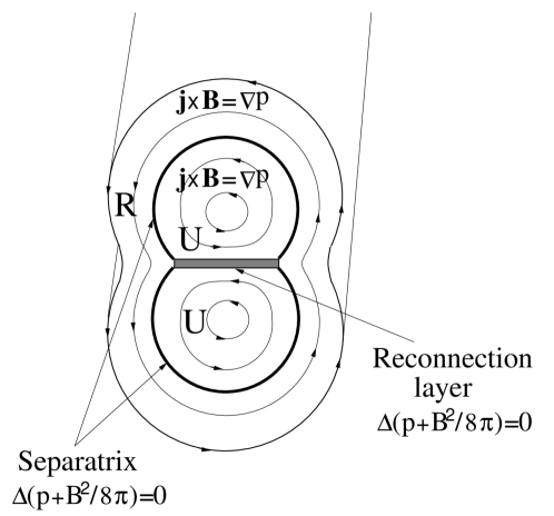
Figure 1: Slow merging of two cylinders. The situation is in a slowly evolving quasistatic equilibrium everywhere, except in the layers across which $p+B^{2}/8\pi$ is continuous. $R$ is the region of reconnected flux, and $U$ is the region of unreconnected flux.

Reconnection is as much a global phenomena as a local one. For example, consider the magnetic reconnection of two cylinders with opposite poloidal flux. (Figure 1.) Let us also assume that the velocities induced by magnetic reconnection are slow compared to the Alfven speed everywhere, except in the reconnection and separatrix layers. Then, everywhere else, we have

$$\bf{j\times B}=\nabla p$$ (1)

Also, since the layers are thin, we have the jump in $p+B^{2}/8\pi$ zero across these layers. This means that, if the amount of reconnected and unreconnected flux is given, and if the rotational transform and pressure are known on each magnetic surface as functions of the poloidal magnetic flux, then there is a unique equilibrium. But as magnetic reconnection proceeds, one can keep track of the pressure and the rotational transform in both the regions of reconnected and unreconnected flux. The two regions change geometrically and physically as reconnection proceeds, Thus, the plasma first moves from the unreconnected region into the reconnection layer, where it is heated, then it flows into the separatrix region, and, finally, as the magnetic configuration changes, into the reconnected region. (However, this does not change the uniqueness of the equilibrium at each stage of reconnection.)

Because of this uniqueness, the length of the reconnection layer $L$ is totally determined at each stage as well as the horizontal field just outside of the layer.

Appreciating this fact, all three authors took the length of the layer as well as the variation of the bounding field as given. They assumed that the region into which the plasma flowed (the separatrix region) was at the same pressure as the upstream ambient pressure. This was the boundary layer problem to be solved.

3 The Sweet-Parker and Petschek Theories for a Constant Resistivity

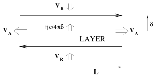
Figure 2: The Sweet-Parker layer. In a steady state the magnetic diffusion velocity $\eta c/4\pi\delta$ balances the incoming reconnection velocity $V_{R}$, and the inflowing mass $4V_{R}L$ balances the outgoing mass $4\delta V_{A}$.

Let us now examine the two theories. First consider that of Sweet and Parker. The reconnection layer is sketched in figure 2. It is easily shown that the flow out of the layer is at the Alfven speed, $V_{x}=V_{A}\equiv B_{0}/\sqrt{4\pi\rho}$. The incoming flow of matter $-LV_{y}=LV_{R}$ must balance the outgoing flow $V_{A}\delta$, where $V_{R}$, the reconnection velocity, is the incoming velocity outside of the layer, where the plasma is tied to the field lines. $\delta$ is the half thickness of the layer. Thus,

$$V_{R}L=V_{A}\delta.$$ (2)

On the other hand, by Ohm’s law the field diffuses up stream with a velocity $\eta c/4\pi\delta$ with respect to the incoming plasma, with velocity $-V_{R}$. Thus, in steady state,

$$V_{R}=\eta c/4\pi\delta.$$ (3)

From these equations we obtain

$$V_{R}=\sqrt{\frac{V_{A}\eta c}{4\pi L}}=\frac{V_{A}}{S},$$ (4)

and

$$\delta=\frac{L}{\sqrt{S}},$$ (5)

where

$$S=\frac{LV_{A}}{\eta c/4\pi}.$$ (6)

This is the Sweet-Parker result.

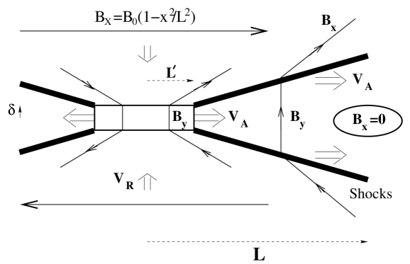
Figure 3: The Petschek model. The diffusion region of length $L^{\prime}<L$ is the same as figure 2, with $L$ taken equal to $L^{\prime}$. Outside the diffusive region   shocks accelerate the plasma and reduce $v_{x}$ to zero. The shocks’ $y$ velocity $B_{y}/\sqrt{4\pi\rho}$ balances the incoming $V_{R}$ velocity in a steady state. The $B_{y}$ field is vital to this model.

The Petschek theory is indicated in figure 3. In this model the diffusive region, in which the merging actually takes place is of a much shorter, length $L^{\prime}$, than $L$. The remaining length of the boundary is occupied by slow shocks. In the diffusive layer the behavior is similar to the Sweet-Parker layer, the main difference being that the acceleration of the velocity up to the Alfven speed along the layer, is accomplished by magnetic tension associated with a transverse field component $B_{y}$. (In the Sweet-Parker theory this acceleration is produced mainly by a pressure gradient.) Outside of the Petschek diffusive layer the acceleration up to $V_{A}$ is accomplished almost instantaneously by the slow shocks. The Sweet-Parker model for their diffusive layer is replaced by the identical conditions for the Petschek model, but with $L$ replaced by $L^{\prime}$, leading to the Petschek reconnection velocity,

$$V_{R}=\sqrt{\frac{V_{A}\eta c}{4\pi L^{\prime}}}=\frac{V_{A}}{\sqrt{S}}\sqrt{\frac{L}{L^{\prime}}},$$ (7)

a factor of $\sqrt{L/L^{\prime}}$ faster than the Sweet-Parker reconnection velocity. The shocks in the outer $L-L^{\prime}$ region reduce the upstream $B_{x}$ to zero, and accelerate the plasma crossing them to $V_{A}$ in the $x$ direction to match the plasma flowing out of the diffusive region with the same Alfven $x$ velocity.

The shocks propagate in the $y$ direction upstream into the plasma with velocity $B_{y}/\sqrt{4\pi\rho}$. Since the plasma is flowing with the reconnection velocity $V_{y}=-V_{A}$ we have in steady state,

$$\frac{B_{y}}{\sqrt{4\pi\rho}}=V_{R},$$ (8)

which determines the magnitude of $B_{y}$ the transverse field component. This $y$ component of the field increases linearly along $x$ in the diffusive region from $0$ to this value, and it turns out that the tension produced by the $j_{z}B_{y}$ force is just enough to accelerate the plasma in the layer up to the Alfven speed.

These results are all given in Petschek’s paper and present a nearly complete, but qualitative, physical picture for magnetic reconnection, encompassing the possibility of a diffusive layer much shorter than $L$. Further, in his theory, $L^{\prime}$ appears to be a free parameter. Petschek then chooses $L^{\prime}$ as short as possible to get the maximum reconnection velocity. He determined this minimum to be the lower limit so that the current in the shocks did not seriously perturb the incoming magnetic field $B_{x}=B_{0}$. This limit was roughly

$$L^{\prime}>\frac{L}{S}(\ln{S})^{2},$$ (9)

so that substituting in equation (7) he got a very fast limit on the reconnection velocity

$$V_{R}<\frac{V_{A}}{\ln{S}}.$$ (10)

This latter limiting velocity has been generally quoted in the literature as the so-called Petschek reconnection velocity, and it is this velocity that has been compared with the Sweet-Parker reconnection velocity equation (4) in the controversy between the two theories. The disagreement should more appropriately be between the Sweet-Parker velocity and equation (7).

Now, it turns out that $L^{\prime}$ is not a free parameter in Petschek’s theory. There is an additional condition associated with $B_{y}$ that Petschek did not include . The all important $B_{y}$ field, which is needed to support the shocks, is embedded in the rapidly moving plasma and is swept down stream at the Alfven velocity, $V_{A}$. This field which is being swept away so rapidly must be regenerated at the same rate to preserve a steady state.

This regeneration occurs during the merging process. The external field is nonuniform, being strongest near $x=0$, so the lines of force at the center of the diffusive layer will move into the diffusive region fastest there. However, the nonuniformity of the external field is on the scale of the length of the layer $L$ because of the global conditions, so as $L^{\prime}$ gets smaller, the nonuniformity over the shorter length is also smaller, and the regeneration process is weaker. A balance between the nonuniform merging process that creates the $B_{y}$ field, and the down sweeping which destroys it, must be reached and this leads to a relation between $L^{\prime}$ and $B_{y}$. Thus, combining this relation with equations (7) and (8), determines $L^{\prime}$ uniquely.

Let us estimate this balance qualitatively. The equation for $B_{y}$ will be shown to be

$$\frac{dB_{y}}{dt}=\frac{V_{R}}{L^{\prime}}\frac{L^{\prime 2}}{L^{2}}B_{0}-B_{y}\frac{V_{A}}{L^{\prime}}=0.$$ (11)

The second term on the right is the down sweeping term that destroys $B_{y}$. Its form is obvious.

The first term represents nonuniform merging, and its form can be derived as follows: (see Figure 4).

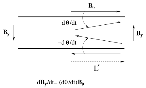
Figure 4: Regeneration of the $B_{y}$ field by nonuniform merging. This rotates the $B_{x}$ field into the $y$ direction.

The external field depends on $x$ as

$$B_{x}=B_{0}(1-x^{2}/L^{2}).$$ (12)

We assume that each fresh line that is merging enters the layer with velocity, $V^{\prime}_{x}$ proportional to $B_{x}(x)$, so that the line enters faster at $x=0$ than at $x=L^{\prime}$. Thus, after entering the layer it will turn at the rate

$$\frac{d\theta}{dt}=\frac{V^{\prime}_{x}(0)-V^{\prime}_{x}(L^{\prime})}{L^{\prime}}=\frac{\eta c}{4\pi\delta L^{\prime}}[1-(1-L^{\prime 2}/L^{2})],$$ (13)

or

$$\frac{d\theta}{dt}=\frac{\eta c}{4\pi\delta}\frac{L^{\prime 2}}{L^{2}}\frac{1}{L^{\prime}}.$$ (14)

The turning of a line of strength $B_{0}$ at the rate $d\theta/dt$ produces a component $B_{y}$ at the rate $(d\theta/dt)B_{0}=V_{R}(L^{\prime 2}/L^{2})B_{0}/L^{\prime}$, which gives the first term in equation(11).

Now, setting $dB_{y}/dt=0$, for a steady state, gives from equation(9),

$$B_{y}=\frac{V_{R}}{V_{A}}(L^{\prime 2}/L^{2})B_{0}.$$ (15)

From equation (8) we get

$$V_{R}=\frac{V_{R}}{V_{A}}(L^{\prime 2}/L^{2})\frac{B_{0}}{\sqrt{4\pi\rho}}=V_{R}(L^{\prime 2}/L^{2}).$$ (16)

or,

$$L^{\prime}=L$$ (17)

.

Thus, $L^{\prime}$ is no smaller than $L$, and the Petschek rate equation (7) reduces to the Sweet-Parker rate equation (4).

I believe that this is the reason that the numerical simulations always yield the Sweet-Parker rate, rather than the faster rate implied by Petschek’s formula.

A more formal derivation of equation (11) is given in the appendix.

4 Anomalous Resistivity in the Sweet-Parker Model

In the absence of a $B_{z}$ component (that is no guide field), there is a strong instability, the lower hybrid instability, that should be excited, (Davidson 1975) This is the case if the current density in the layer is large enough that the difference in the electron and ion bulk velocities $v_{-}$ and $v_{+}$ is greater than the ion acoustic speed. That is, if the drift velocity $v_{d}\equiv v_{+}-v_{-}$ satisfies $v_{d}>v_{i}$ with $v_{i}$ the ion thermal velocity. Note that $j=n_{e}(e/c)v_{d}$.

There are three well-documented instances where magnetic reconnection is definitely taking place, i.e. the solar flare, the magnetosphere-solar wind interface, and the magnetotail. If one examines these three cases, and applies the Sweet-Parker model to them, one finds in all three cases that the drift velocity, $v_{d}$, is much larger than $v_{i}$. One can express this as follows: There is a critical current, $j_{c}$, and critical layer thickness $\delta_{c}=B_{0}/4\pi j_{c}$ such that if $\delta<\delta_{c}$ and therefore $j$ is greater than the critical $j$, then the lower hybrid mode should be excited. This lower hybrid instability has the property, that it can generate an almost unlimited amount of resistive friction between the electrons and the waves.

Now, let us imagine the two plasmas with opposite magnetic fields, $B_{0}$, approach each other. The pressure, between them, $p=B_{0}^{2}/8\pi$, is dissipated at the rate $V_{A}/L$ by expansion due to flow out the ends, and by force balance, must be replenished by compression due to $d\delta/dt<0$. This compression normally continues until the Sweet-Parker thickness is reached. At this time, the plasma pressure in the layer is replenished by Ohmic heating $\eta j^{2}\approx\eta B_{0}^{2}/(4\pi\delta)^{2}$ at the same rate at which it is depleted, $(V_{A}/L)p=(V_{A}/L)(B_{0}^{2}/8\pi)$, by the adiabatic expansion. Therefore at this time the collapse $d\delta/dt$ ceases.

On the other hand, if the critical thickness, $\delta_{c}$, is passed before the Sweet-Parker thickness is reached, the resistivity rapidly rises to generate an Ohmic heating large enough to balance the outflow adiabatic expansion at this larger distance $\delta_{c}$, and collapse ceases at this larger distance.

For these conditions, the layer thickness is known, and $V_{R}$ is determined by the mass conservation equation (2) alone,

$$V_{R}=\frac{\delta_{c}}{L}V_{A}.$$ (18)

Thus, reconnection can become much faster than the Sweet-Parker rate based on Spitzer resistivity. Under solar flare conditions, Kulsrud (1998), it can become as much as a factor of a thousand faster. The resulting reconnection time can be reduced to a few hours, perhaps an order of magnitude longer than the observed energy release time in solar flares.

5 Petschek Reconnection with Anomalous Resistivity

In the second section it was shown that for a constant resistivity, Petschek’s $L^{\prime}$ parameter must be equal to $L$, so that Petschek’s reconnection rate reduces to that of Sweet-Parker. However, if $\eta$ is anomalous, enhanced by wave interactions, it can be very sensitive to the current density. The original problem with Petschek reconnection was that the external field at $x=L^{\prime}$ was only slightly smaller, by a factor of $1-L^{\prime 2}/L^{2}$, than its strength at $x=0$. But even this slight change in the resulting current density can lead to a finite and even large change in the resistivity $\eta$. Taking this into account, one finds that equation (11) becomes

$$\frac{d\theta}{dt}=\frac{\eta_{0}c}{4\pi\delta L^{\prime}}-\frac{\eta^{\prime}c}{4\pi\delta^{\prime}L^{\prime}}(1-\frac{L^{\prime 2}}{L^{2}})\approx\frac{(\eta_{0}-\eta^{\prime})c}{4\pi\delta L^{\prime}},$$ (19)

in which we have neglected $L^{\prime 2}/L^{2}$ and any slight difference between $\delta$ and $\delta^{\prime}$. $\eta_{0}$ is the resistivity at $x=0$, and $\eta^{\prime}$ that at $x=L^{\prime}$. Solving for $B_{y}=(d\theta/dt)B_{0}$ as before, with this different value of $d\theta/dt$, and using it in Petschek’s formula for the shock velocity, we find that with variable resistivity,

$$V_{R}=\frac{B_{y}}{\sqrt{4\pi\rho}}=\frac{1}{V_{A}}\frac{B_{0}}{\sqrt{4\pi\rho}}\frac{(\eta_{0}-\eta^{\prime})c}{4\pi\delta}.$$ (20)

Taking $\delta=\delta_{c}$, we have

$$V_{R}=\frac{c(\eta_{0}-\eta^{\prime})}{4\pi\delta_{c}}.$$ (21)

Now, to estimate the value of this revised reconnection velocity, we assume that $\eta$ is linear in $j$ for $j>j_{c}$, so that

$$\eta_{0}-\eta^{\prime}=(j_{0}-j^{\prime})\frac{d\eta}{dj}=\frac{1}{4\pi}(\frac{B_{0}}{\delta}-\frac{B^{\prime}}{\delta^{\prime}})\frac{d\eta}{dj}=\frac{1}{4\pi}\frac{L^{\prime 2}}{L^{2}}\frac{B_{0}}{\delta_{c}}\frac{d\eta}{dj}$$ (22)

Combining this with the mass conservation relation for the $L^{\prime}$ layer,

$$\frac{V_{R}}{V_{A}}=\frac{\delta_{c}}{L^{\prime}},$$ (23)

we obtain

$$\frac{V_{R}^{3}}{V_{A}^{3}}=\frac{B_{0}}{V_{A}L^{2}}\frac{c}{(4\pi)^{2}}\frac{d\eta}{dj}.$$ (24)

This result can be written in a more familiar way by assigning a maximum value, $\eta^{*}$ to $\eta$ and assuming that $\eta=\eta_{spitzer}$ for $j<j_{c}$, and $\eta=\eta^{*}$ at $j=2j_{c}$. Thus,

$$\frac{d\eta}{dj}=\frac{\eta^{*}}{j_{c}}.$$ (25)

From $j_{c}=B_{0}/4\pi\delta_{c}$ equation (24) reduces to

$$\frac{V_{R}}{V_{A}}=\left(\frac{\delta_{c}}{L}\frac{1}{S^{*}}\right)^{1/3},$$ (26)

where $S^{*}$ is the modified Lundqvist number based on $\eta^{*}$

$$S^{*}=\frac{V_{A}L}{\eta^{*}c/4\pi}$$ (27)

Numerically, $\eta^{*}$ comes from an electron wave collision rate equal to the electron plasma frequency $\omega_{pe}$. Under typical solar flare conditions, Kulsrud (1998), $\eta^{*}\approx 10^{6}\eta_{Spitzer}$, and

$$\frac{V_{R}}{V_{A}}\approx 10^{-4}$$ (28)

One can carry out similar estimates for the magnetosphere-solar wind interface and one finds from equation (26) that

$$\frac{V_{R}}{V_{A}}\approx 10^{0}$$ (29)

6 Conclusions

We have shown or stated that:

(1). In general reconnection situations, $L$ and $B_{x}$ are determined globally, while $\delta$ and $V_{R}$ are determined locally.

(2). For constant resistivity, the length of Petschek’s diffusive layer is not a free parameter, but is determined by the condition that $B_{y}$ be regenerated at the same rate as it is being dissipated by down stream flow.

(3).Constant resistivity gives $L^{\prime}=L$, which makes Petschek’s reconnection rate equal to that of Sweet and Parker.

(4). If the Sweet-Parker thickness $\delta=L/\sqrt{S}$ is thinner than the critical thickness $\delta_{c}$ at which anomalous resistivity sets in, then the Sweet Parker reconnection rate becomes

$$V_{R}=\frac{\delta_{c}}{L}V_{A},$$ (30)

a rate that can be very much faster than their reconnection rate based on Spitzer resistivity.

(5). In the case of anomalous resistivity the regeneration rate of $B_{y}$ in Petschek’s theory is much larger, and the Petschek’s rate becomes faster even than the Sweet-Parker rate with enhanced resistivity. It is given by

$$\frac{V_{R}}{V_{A}}=\left(\frac{\delta_{c}}{L}\frac{1}{S^{*}}\right)^{1/3}$$ (31)

where $S^{*}=LV_{A}/(\eta^{*}c/4\pi)$ is the Lundqvist number based on the maximum possible resistivity $\eta^{*}$. Note that it has a cube root dependence on this maximum resistivity, rather than a logarithmic dependence on the Spitzer resistivity which is the often quoted expression for Petschek reconnection. In spite of this, in many cases there is not a large numerical difference in the two results. Formula (31) gives an equally fast reconnection rate, and is more in tune with the true physical processes.

(6). A test for whether the anomalous resistivity rate equation (18) or (31), rather than the classical Sweet-Parker rate, equation (7), is applicable is: First, compute the Sweet-Parker thickness $\delta_{SP}$, of the reconnection layer $\delta_{SP}=L/\sqrt{S}$, and compare it with the critical thickness $\delta_{c}=B_{0}/(4\pi n_{e}v_{i}/c)$. If $\delta_{SP}<\delta_{c}$, then use the anomalous equation (31) for Petschek reconnection, or the anomalous Sweet-Parker equation (18), whichever is faster.

(7). In nearly all cases on the galactic scale, $\delta_{SP}$ is larger than or at least comparable to $\delta_{c}$, so the Sweet-Parker result gives the correct order of magnitude for the reconnection rate. This is almost always too slow to be of interest, so one concludes that reconnection on the galactic scale is hardly ever really important.

7 Acknowledgment

I gratefully acknowledge many useful discussions with my colleagues, Dmitri Uzdensky, Masaaki Yamada and Hantao Ji. I am also very grateful for much help from Leonid Malyshkin in preparing the manuscript for publication.

Appendix

In this appendix we justify the intuitively described equation (11) for the evolution $B_{y}$, by a more precise derivation. In the intuitive derivation, it was assumed that the lines flowed into the reconnection only by resistive merging, and the effect of plasma flow on them was ignored. Also, the merging velocity was taken proportional to the external field, through its effect on the current density. Further, the thickness of the reconnection layer was assumed constant between $x=0$ and $x=L^{\prime}$.

Consider an $x$ dependent thickness $\delta(x)$, as shown in figure 5, taken large enough that at $y=\delta(x),B_{x}\approx B(x)=B_{0}(1-x^{2}/L^{2})$, the value for the external field. Also take $\delta(x)$ to follow a line of force. We have Ohm’s law in the layer,

$$-cE_{z}=-V_{y}B_{x}+V_{x}B_{y}-\eta cj_{z}.$$ (A1)

In a steady state $E_{z}$ is a constant.

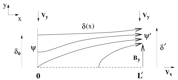
Figure 5: Sketch of the Petschek diffusion layer for the $B_{y}$ field derivation. At $x=L^{\prime},B_{x}$ is zero nearly up to $y=\delta^{\prime}$. $\delta(x)$ is a line of force.

Integrate $-cE_{z}$ at $x=0$, from $y=0$ to $y=\delta_{0}=\delta(0)$. See figure 5. Since $B_{y}=0$ at $x=0$, we have

$$c\int_{0}^{\delta_{0}}-E_{z}dy=\int_{0}^{\delta_{0}}-v_{y}B_{x}dy+\eta c\int_{0}^{\delta_{0}}-j_{z}dy,$$ (A2)

or

$$c\int_{0}^{\delta_{0}}-E_{z}dy=\int_{0}^{\delta_{0}}-v_{y}B_{x}dy+\frac{\eta c}{4\pi}\int_{0}^{\delta_{0}}\frac{\partial B_{x}}{\partial y}dy,$$ (A3)

or

$$c\int_{0}^{\delta_{0}}-E_{z}dy=\int_{0}^{\delta_{0}}-v_{y}B_{x}dy+\frac{\eta c}{4\pi}B_{0}.$$ (A4)

Note that $-E_{z},-V_{y}$, and $-j_{z}$ are positive.

Correspondingly, integrate $-E_{z}$ at $x=L^{\prime}$, from $y=0$ to $y=\delta^{\prime}=\delta(L^{\prime})$,

$$c\int_{0}^{\delta^{\prime}}-E_{z}dy=\int_{0}^{\delta^{\prime}}-v_{y}B_{x}dy+\int_{0}^{\delta^{\prime}}v_{x}B_{y}dy+\frac{\eta c}{4\pi}B_{0}(1-L^{\prime 2}/L^{2}).$$ (A5)

At large enough $\delta$, we have

$$-V_{y}(0,\delta_{0})=V_{R},$$ (A6)

and

$$-V_{y}(L^{\prime},\delta^{\prime})=\frac{V_{R}B_{0}}{B_{0}(1-L^{\prime 2}/L^{2})},$$ (A7)

since $y=\delta(x)$ is in the infinitely conducting region, and

$$-cE_{z}=-V_{y}(0,\delta_{0})B_{x}(0,\delta_{0})=-V_{y}(L^{\prime},\delta^{\prime})B_{x}(L^{\prime},\delta^{\prime}).$$ (A8)

But, because $E_{z}$ is constant for all $x$ and $y$, the left hand side of equation (A4) and (A5) are equal to $-cE_{z}\delta_{0}$ and $-cE_{z}\delta^{\prime}$, respectively. Therefore, subtracting the right hand side of equation (A5) from $\delta^{\prime}/\delta_{0}$ times that of equation (A4), we get

$$\frac{\delta^{\prime}}{\delta_{0}}\int_{0}^{\delta_{0}}-v_{y}B_{x}dy-\int_{0}^{\delta^{\prime}}-v_{y}B_{x}dy+\frac{\eta c}{4\pi}\left[\frac{\delta^{\prime}}{\delta_{0}}B_{0}-B_{0}(1-\frac{L^{\prime 2}}{L^{2}})\right]=\int_{0}^{\delta^{\prime}}-v_{y}B_{x}dy.$$ (A9)

The third term on the left hand side, the $\eta$ term, is the non uniform merging term quoted in the text. In fact, we can write it as $\alpha(\eta c/4\pi)(B_{0}/\delta_{0})(L^{\prime 2}/L^{2})$ where $\alpha$ is a constant of order unity and equal to $1+(1/2)d^{2}\delta/dx^{2}$, which includes the change of $\delta(x)$ with respect to $x$. The right hand side represents the down sweeping term which destroys $B_{y}$.

We now argue that the sum of the first two terms on the left hand side is negative, so that the expression in the text for $B_{y}$ should be an inequality rather than an equality. Since this is partially compensated by the fact that the regeneration term is slightly larger, by the factor of $\alpha>1$, we work with equality in the main text.

First, the mean value of $-V_{y}$ in the first term, weighted by $B_{x}$ is about 2/3 times $-V_{y}(\delta_{0})=V_{R}$ because both $-V_{y}$ and $B_{x}$ are linear in $y$. Thus,

$$\frac{\delta^{\prime}}{\delta_{0}}\int_{0}^{\delta_{0}}-v_{y}B_{x}dy\approx\frac{\delta^{\prime}}{\delta_{0}}\frac{2}{3}V_{R}\psi$$ (A10)

where

$$\psi=\int_{0}^{\delta_{0}}B_{x}dy,$$ (A11)

is the $B_{x}$ flux up to $\delta_{0}$. On the other hand, we see from figure 5 that the entire $B_{x}$ flux at $y=L^{\prime}$ is near $\delta^{\prime}$, so here the $B_{x}$ averaged value of $V_{y}$ is $V_{R}/(1-L^{\prime 2}/L^{2})\approx V_{R}$. Thus the sum of the first two terms in equation (A9) is essentially,

$$\frac{2}{3}\frac{\delta^{\prime}}{\delta_{0}}V_{R}\psi-\frac{V_{R}}{1-L^{\prime 2}/L^{2}}\psi^{\prime}$$ (A12)

where $\psi^{\prime}$ is the $B_{x}$ flux at $y=L^{\prime}$. Further, we also see, from Figure 5, that $\psi^{\prime}$ is greater than $\psi$ because $\psi^{\prime}$ contains the $\psi$ flux (because $\delta(x)$ is a line of force) plus the flux through $y=0$, between $x=0$ and $x=L^{\prime}$. Therefore, if $\delta^{\prime}/\delta<3/2$, a plausible assumption, since $L^{\prime}\ll L$, then the sum in equation (A12) is negative. In addition, the factors $\psi^{\prime}/\psi>1$ and $1/(1-L^{\prime 2}/L^{2})>1$ reinforce the conclusion that the sum is negative.

Now, dropping the first two terms in equation (A9) whose sum has been shown to be negative, we obtain the inequality,

$$\alpha\frac{\eta c}{4\pi}B_{0}\frac{L^{\prime 2}}{L^{2}}>\int_{0}^{\delta_{0}}-v_{x}B_{y}dy\approx V_{A}\delta^{\prime}<B_{y}>$$ (A13)

Comparing this with equation (11) of the text we see that, if $\alpha$ were one, equation (15) would yield an overestimate of $B_{y}$. Since $\alpha$ is certainly of order one, it is safe to take equation (15) as an estimate of $B_{y}$.

Note, that equation (A9) is approximately the rate of change of $L^{\prime}\delta B_{y}$ since

$$\int_{0}^{L^{\prime}}dx\int_{0}^{\delta(x)}dy\frac{\partial B_{y}}{\partial t}=\int\int dxdy\frac{\partial E_{z}}{\partial x}=\delta(x)E_{z}|_{0}^{L^{\prime}},$$ (A14)

and the latter expression can easily be identified with the difference of the two integrals given in equations (A4) and (A5) with the extra $\delta^{\prime}/\delta_{0}$ factor.

References

- [1] Biskamp, D., 1986 Phys. of Fluids, 29, 1520.
- [2] Davidson, R., 1975 Phys. of Fluids 18, 1327.
- [3] Kulsrud, R. M., 1998 Phys. of Plasmas 5, 1599.
- [4] Parker, E., 1957 Phys. Rev. 107, 830.
- [5] Petschek, H. E., 1964, in Physics of Solar Flares, edited by W. N. Ness, NASA Sweet Parker-50 p 425.
- [6] Sweet, P.A., 1958, IAU Symposium No. 6 Electromagnetic Phenomena in Ionized Gases (Stockholm 1956) p. 123.