The evolution of the color gradients of early-type cluster galaxies

Abstract

We investigate the origin of color gradients in cluster early-type galaxies to probe whether pure age or pure metallicity gradients can explain the observed data in local and distant ($z\approx 0.4$) samples. We measure the surface brightness profiles of the 20 brightest early-type galaxies of CL0949+44 (hereafter CL0949) at redshift $z$=0.35-0.38 from HST WF2 frames taken in the filters F555W, F675W, F814W. We determine the color profiles $(V-R)(r)$, $(V-I)(r)$, and $(R-I)(r)$ as a function of the radial distance $r$ in arcsec, and fit logarithmic gradients in the range $-0.2$ to 0.1 mag per decade. These values are similar to what is found locally for the colors $(U-B)$, $(U-V)$, $(B-V)$ which approximately match the $(V-R)$, $(V-I)$, $(R-I)$ at redshift $\approx 0.4$. We analyse the results with up to date stellar population models. We find that passive evolution of metallicity gradients ($\approx 0.2$ dex per radial decade) provides a consistent explanation of the local and distant galaxies’ data. Invoking pure age gradients (with fixed metallicity) to explain local color gradients produces too steep gradients at redshifts $z\approx 0.4$. Pure age gradients are consistent with the data only if large present day ages $\geq 15$ Gyr are assumed for the galaxy centers.

1 Introduction

The efforts to understand the mechanisms of formation and evolution of elliptical galaxies have dramatically increased in the last years. On the theoretical side, the classical picture of the monolithic collapse à la Larson (L74 (1974)) has been increasingly questioned by scenarios of hierarchical structure formation, where ellipticals are formed by mergers of spirals (White & Rees WR78 (1978)). While in the first case the stars of the galaxies are supposed to form in an early episode of violent and rapid formation, the semi-analytical models of galaxy formation (Kauffmann K96 (1996), Baugh et al. Betal96 (1996)) predict more extended star formation histories, with substantial fractions of the stellar population formed at relatively small redshifts. From an observational point of view, evidence is growing that the formation of a fair fraction of the stellar component of bright cluster Es must have taken place at high redshift ($z\geq 2$) and cannot have lasted for more than 1 Gyr. This conclusion is supported at small redshifts by the existence of a number of correlations between the global parameters of elliptical galaxies, all with small scatter: the Color-Magnitude (CM, Bower et al. Betal92 (1992)), the Fundamental Plane (Jørgensen et al. JFK96 (1996)), the Mg-$\sigma$ (Colless et al. Cetal99 (1999)) relations. These hold to redshifts up to 1 (Stanford et al. SED98 (1998), Bender et al. BSZBBGH97 (1998), Kelson et al. KDFIF97 (1997), van Dokkum et al. DFKI98 (1998), Bender, Ziegler & Bruzual BZB96 (1996), Ziegler & Bender ZB97 (1997), Ellis et al. Eetal97 (1997)), consistent with passive evolution and high formation-ages. In addition, the Mg over Fe overabundance of the stellar populations of local cluster Es (Worthey, Faber & González WFG92 (1992), Mehlert et al. 2000b ), requires short star formation times and/or a flat IMF (Thomas, Greggio, Bender TGB99 (1999)). Field ellipticals might have larger spreads in formation ages (Gonzáles G93 (1993)), but comparisons with cluster Es (Bernardi et al. Betal98 (1998)) and the first trends observed for the evolution of the FP with redshift (Treu et al. T99 (1999)) do not allow much freedom.

The study of the variations of the stellar populations inside galaxies, the so-called gradients, offers an additional tool to constrain the models of galaxy formation. Classical monolithic collapse models with Salpeter IMF (Carlberg C84 (1984)) predict strong metallicity gradients. The merger trees generated by hierarchical models of galaxy formation (Lacey & Cole LC93 (1993)) are expected to dilute gradients originally present in the merging galaxies and therefore give end-products with milder gradients (White W80 (1980)), although detailed quantitative predictions are still lacking. Color gradients are known to exist in ellipticals since the pioneering work of de Vaucouleurs (dV61 (1961)). The largest modern, CCD based, dataset has been collected by Franx et al. (FIH89 (1989)), Peletier et al. (PDIDC90 (1990)), Goudfrooij et al. (GHJNDV94 (1994)), who measured surface brightness profiles in the optical $U,\leavevmode\nobreak\ B,\leavevmode\nobreak\ V,\leavevmode\nobreak\ R,\leavevmode\nobreak\ I$ bands for a large set of local ellipticals. These radial changes in colors have been traditionally interpreted as changes in metallicity (Faber F77 (1977)), arguing that line index gradients measured in local field (Davies et al. D93 (1993), Carollo et al. C93 (1993), Kobayashi & Arimoto KA99 (1999)) and cluster (Mehlert et al. M98 (1998), 2000a ) galaxies support this view. A $\approx 0.2$ dex change in metallicity per radial decade suffices to explain the photometric and spectroscopic data (see, for example, Peletier et al. PDIDC90 (1990)). However, due to the age-metallicity degeneracy of the spectra of simple stellar populations (Worthey W94 (1994)) this conclusion can be questioned. De Jong (dJ96 (1996)) favors radial variations in age to explain the color gradients observed in his sample of local spiral galaxies. If ellipticals form from merging of spirals, age might be the driver of color gradients in these objects too. The combined analysis of more metal-sensitive (i.e., Mg₂) and more age-sensitive (i.e., $H\beta$) line index profiles points to a combination of both age and metallicity variations (Gonzáles G93 (1993), Mehlert et al. 2000b ). Finally, Goudfrooij & de Jong (GdJ95 (1995)) and Wise & Silva (WS96 (1996)) stress the importance of dust on the interpretation of color gradients and conclude that it might add an additional source of degeneracy to the problem.

With the resolution power of HST it is now possible to measure the photometric properties of distant galaxies and therefore implement an additional constraint on the stellar population models, i.e. the time evolution, that helps breaking the degeneracies discussed above. Abraham et al. (AEFTG99 (1999)) study color distributions of intermediate redshift galaxies of the Hubble Deep Field to constrain the star formation history of the Hubble Sequence of field galaxies. Here we determine the color gradients in the $V,\leavevmode\nobreak\ R,\leavevmode\nobreak\ I$ Johnson-Cousins filters of a sample of cluster early-type galaxies at redshift $z\approx 0.4$ observed with HST, and compare them to the U, B and V gradients observed in local Es. By means of new, up to date models of Simple Stellar Populations (SSP), we investigate whether pure age or pure metallicity gradients can explain the observed colors and gradients and their evolution with redshift. The structure of the paper is the following. In Sect. 2 we present the new HST observations of CL0949, the data reduction and the derived photometric profiles. In Sect. 3 we describe the reference sample of local cluster galaxies. In Sect. 4 we describe the stellar population models and their use to study the evolution of color gradients. Ages and metallicities derived according to the different modeling assumptions are presented in Sect. 5. Results are discussed in Sect. 6 and conclusions are drawn in Sect. 7.

2 HST Observations of CL0949

The central core of CL0949 (a superposition of two clusters at redshifts 0.35 and 0.38, Dressler & Gunn DG92 (1992)) was observed with HST and WFPC2 in December 1998 (PID 6478). Nine images with each of the filters F555W, F675W, and F814W were obtained totaling exposure times of 7200 sec, 7200 sec, and 7000 sec respectively. The images were taken with sub-pixel shifts to improve the resolution and sampling. The pipeline reduced frames were further processed under IRAF to eliminate cosmic rays, and combined after resampling to half the original scale, following the algorithm described in Seitz et al. (SSBHBZ98 (1998)). The subsequent analysis was performed under MIDAS. Particular care was needed to treat the images taken with the filter F555W, which suffered from an elevated background level throughout the field of view, due to Earth reflection by the optical telescope assembly and spiders, and the related presence of a dark diagonal X structure. In order to determine the background accurately, the Sextractor program (Bertin & Arnoux BA96 (1996)) was used. We detected and subtracted sources iteratively and constructed an average source-free sky frame. The resulting source-free, sky-subtracted images taken with the F675W and F814W filters have rms residuals of 0.3-0.5%, the ones with the F555W filter up to 1%, which set the final precision of our sky subtraction. In addition, we constructed background-subtracted images using the first-iteration background determined by Sextractor, which takes into account the diffuse light contribution of extended objects. These frames were then used to perform the surface photometry analysis for all galaxies except for the cD on the WF2 frame (#201 of Fig. 1). In this case we preferred the sky-subtracted images to be able to measure the extended halo of the object.

Figure 1: The F814W image of the cluster CL0949. The labels indicate the 20 brightest early-type galaxies detected.

The isophote shape analysis was performed following Bender and Möllenhoff (BM87 (1987)). The procedure was improved in two aspects. 1) Mask files were produced automatically from the “segmentation frames” produced by Sextractor. 2) The surface brightness and integrated magnitude profiles following elliptical isophotes were computed from the averages of the not masked pixels between the isophotes. Statistical errors were also derived from the measured rms. Profiles of surface brightness, ellipticity, position angle and higher order terms of the Fourier decomposition were derived for the 70 brightest objects detected by Sextractor on the F814W frames. The information was used in combination with the visual inspection of the images to classify the galaxies morphologically. Twenty early-type galaxies were found. Their identification numbers can be read in Fig. 1. In the following we shall consider only these objects. The data for the late-type galaxies will be presented elsewhere. The cross-identification with Dressler & Gunn (DG92 (1992)) is given in Table 1, where the available spectroscopic information is also summarized. Inspection of the profiles of the isophote shape parameters shows smooth variations as a function of the radial distance, and absence of strong odd-term coefficients, which excludes the presence of large amounts of patchy dust. This is confirmed by the examination of the two-dimensional (V-R), (V-I), (R-I) color maps.

Table 1: Results of the photometric fits. Column 1 gives the galaxy name (see Fig. 1), Col. 2 the cross identification with Dressler & Gunn (DG92 (1992)), Col. 3 the redshift from Dressler & Gunn (DG92 (1992)), Col. 4 the morphological type, Cols. 5-10 give the half-luminosity radii $R_{e}$ in arcsec and total magnitudes $m_{T}$ in the F555W, F675W, and F814W filters respectively. Magnitudes are calibrated to the $V,\leavevmode\nobreak\ R,\leavevmode\nobreak\ I$ Johnson-Cousins system (see text). Col. 11 gives the central velocity dispersions from Ziegler & Bender (ZB97 (1997)) and comments.

Name	D&G92	z	Type	$R_{e}(555)$	$m_{T}(555)$	$R_{e}(675)$	$m_{T}(675)$	$R_{e}(814)$	$m_{T}(814)$	Comment
201	118	.3815	cD	1.46	19.44	1.901	18.061	2.051	17.231	$\sigma=325\pm 50$
202			E	0.64	20.54	0.59	19.53	0.55	18.78
203	102	.3766	SB0	0.35	20.52	0.37	19.58	0.36	18.87	E+A
204	130	.3402	E	0.63	20.77	0.58	19.85	0.55	19.09
205			E/S0	0.52	20.91	0.49	19.86	0.48	19.08
206			E	0.72	20.84	0.58	19.91	0.54	19.17
208	123	.3779	S0	0.45	21.51	0.47	20.4	0.50	19.58
209	110	.3744	S/S0	0.67	21.3	0.66	20.34	0.62	19.74
210			E/S0	0.44	21.45	0.34	20.51	0.41	19.69
211	108	.3799	E/S0	0.20	21.87	0.18	20.79	0.20	20.03
302	163	.3778	E/S0	0.65	20.42	0.58	19.47	0.57	18.70
303	119	.3484	E/S0	0.43	21	0.49	19.88	0.44	19.17
304			S0	0.56	21.1	0.47	20.11	0.48	19.31
312			E/S0	0.15	22.5	0.16	21.39	0.15	20.67
401	221	.3772	E	1.07	20.05	1.05	18.87	1.07	18.06	$\sigma=230\pm 25$
402	193	.3767	Sa/S0	1.12	20	1.10	18.93	1.12	18.14	$\sigma=230\pm 25$
403	217	.3784	E	0.69	20.42	0.71	19.32	0.69	18.57	$\sigma=125\pm 15$
404	187	.3778	E	0.81	20.63	0.77	19.61	0.76	18.87
405			SB0	0.37	21.79	0.29	20.83	0.29	20.05
408			S0	$-^{2}$	$-^{2}$	1.03	20.7	0.85	19.78	Background?
1: uncertain
2: profile too short to allow a reliable fit

Circularly averaged surface brightness profiles were also measured following Saglia et al. (1997a ). The photometric calibration on the $V,\leavevmode\nobreak\ R,\leavevmode\nobreak\ I$ Johnson-Cousins bands was performed using the “synthetic system” (Holzmann et al. HBCHTWW95 (1995)) as in Fig. 1 of Ziegler et al. (ZSBBGS99 (1999)). A first estimate of the zero-points was obtained using the $(V-I)$ and $(V-R)$ colors typical of $z=0.4$ early-type galaxies, as in Ziegler et al. (ZSBBGS99 (1999)). The final zero-points were derived recomputing the calibration with the so-measured $(V-I)$ and $(V-R)$ colors. Half-luminosity radii $R_{e}(555)$, $R_{e}(675)$, $R_{e}(814)$ and total magnitudes $m_{T}(555)$, $m_{T}(675)$, $m_{T}(814)$ were derived fitting the circularly averaged profiles using the algorithm described and extensively tested in Saglia et al. (1997b ). The algorithm fits a PSF (computed using the Tinytim program) broadened $r^{1/4}$ and an exponential component simultaneously and separately to the circularly averaged surface brightness profiles. As a result, disk-to-bulge ratios and the scale-lengths of the bulge and the disk components are also determined. The quality of the fits were explored by Monte Carlo simulations in Saglia et al. (1997b ), taking into account the possible influence of sky subtraction errors, the signal-to-noise ratio, the radial extent of the profiles and the $\chi^{2}$ quality of the fit. Accordingly, the half-luminosity radii are expected to be accurate to 25%, the total magnitudes to 0.15 mag. Two fits are more uncertain than these figures. The values of $R_{e}(814)$ and $R_{e}(675)$ of galaxy 201 have been derived restricting the fit to the radial range of the F555W profile. Fitting the whole F814W profile, more extended than the F555W and F675W ones and shallower than the extrapolated profiles expected from the fits in the V and R bands, one would get a value of $R_{e}(814)$ twice as large. Fitting the whole F675W profile produces a value of $R_{e}(675)$ 30% smaller. Finally, the F555W profile of the galaxy 408 is not extended enough to allow a reliable determination of $R_{e}(555)$. The best fit the these data involves a large (50%) extrapolation and gives a value of $R_{e}(555)$ twice as large as $R_{e}(675)$ and $R_{e}(814)$.

Fig. 2 shows the resulting fits to the F814W filter profiles and the profiles in the F675W and F555W bands.

Half-luminosity radii and total magnitudes are given in Table 1. The scales ($R_{eB}$ and $h$ in arcsec) and the magnitudes ($m_{B}$ and $m_{D}$) of the bulge and disk components measured with the F814W profiles are given in Table 2 together with the $D/B$ ratio, for the objects where a two-component model was fit. As described above, the fit to the galaxy 201 is highly uncertain. If the whole radial extent of the F814W profile is fit, an 8 times larger value of the bulge scalelength is needed.

Following Burstein & Heiles (BH84 (1984)), no correction for galactic absorption was necessary. Note, however, that Schlegel et al. (SFD98 (1998)) give $E(B-V)=0.019$. The use of this correction gives $A_{V}=0.063$, $A_{R}=0.051$, $A_{I}=0.037$, making the derived intrinsic $(V-R)$, $(V-I)$, $(R-I)$ colors bluer by 0.01, 0.026, 0.014 mag respectively. These variations do not affect what follows.

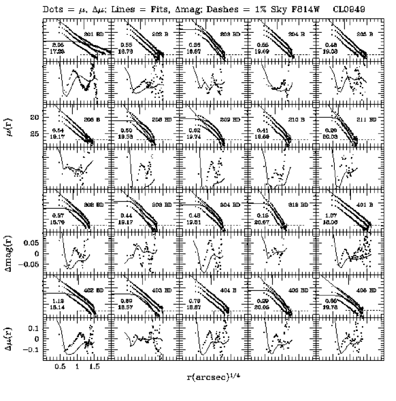
Figure 2: The fits to the circularly averaged surface brightness profiles (taken with the F814W filter and calibrated in the Cousins I band) of the 20 brightest early-type galaxies of CL0949. Two plots are shown for each galaxy. The upper panel shows the calibrated surface brightness profile (small dots) together with the fitted bulge and/or disk profiles (full lines) as a function of the 1/4 power of the distance $r$ from the center in arcsec. The horizontal dashed line shows the position corresponding to 1 per cent of the sky level. We also show the circularly averaged surface brightness profiles taken with the F675W and F555W filters, calibrated in the Johnson-Cousins V and R bands. For clarity they have been shifted by 0.5 and 1 mag respectively. In each panel the galaxy name and the type of best fit are given (B for bulge only, D for disk only, BD for bulge+disk fit), together with the value of $R_{e}$ in arcsec and the total magnitude calibrated in the Cousins I band. The $R_{e}$ location is also marked as a vertical line from the top xaxis in each panel. Below each surface brightness profile we show the residuals of the fits, $\Delta\mu(r)=\mu_{obs}(r)-\mu_{fit}(r)$ (dots, scale -0.2 to 0.2 mag arcsec^-2) and the integrated magnitude difference $\Delta mag(r)=mag_{obs}(<r)-mag_{fit}(<r)$ (full lines, scale -0.1 to 0.1 mag).

Table 2: The parameters of the bulge+disk fits as measured with the F814W profiles. Col. 1 gives the galaxy name (see Fig. 1), Col. 2 the half-light radius of the bulge component $R_{eB}$ in arcsec, Col. 3 the magnitude of the bulge component $m_{B}$, Col. 4 the scalelength $h$ of the disk component in arcsec, Col. 5 the magnitude of the disk component $m_{D}$, Col. 6 the disk-to-bulge ratio $D/B$. Magnitudes are calibrated to the I Cousins filter (see text).

Name	$R_{eB}(814)$	$m_{B}(814)$	$h(814)$	$m_{D}(814)$	$D/B$
2011	0.80	17.81	3.08	18.18	0.71
203	0.44	19.32	0.18	20.05	0.51
208	0.16	20.5	0.48	20.18	1.34
209	0.26	21.42	0.42	20	3.69
211	0.18	20.4	0.14	21.36	0.42
302	0.49	18.89	0.54	20.68	0.19
303	0.60	19.41	0.13	20.92	0.25
304	0.38	19.81	0.36	20.41	0.58
312	0.12	21.13	0.11	21.83	0.53
402	1.02	18.4	0.80	19.82	0.27
403	0.67	18.67	0.45	21.21	0.097
405	0.25	20.48	0.19	21.26	0.49
408	0.82	20.09	0.54	21.3	0.33
1: uncertain fit

Finally, we determined the color profiles of the galaxies from the calibrated elliptical isophote surface brightness profiles, estimating statistical and systematic errors. The latter were computed considering the extreme cases of possible sky subtraction errors, $\pm 0.5$% for the F675W and F814W filters, and $\pm 1$% for the F555W (see above). For example, we computed the two $(V-I)$ profiles corresponding to +1% sky error on V and -0.5% sky error on I, and -1% sky error on V and +0.5% sky error on I. The error budget on the colors is dominated by statistics in the central regions of the galaxies, and by systematics in the outer parts. We fitted the logarithmic slope gradient and zero point, weighting the data according to the statistical errors. In the fit we consider only points within 0.1 ($R_{min}$)and 3.2 ($R_{max}$) arcsec and with statistical and systematic errors less than 0.1 mag. Systematic errors on the gradients and zero-points due to sky subtraction were estimated determining the two quantities for the two extreme cases of possible sky errors discussed above. The median value of $R_{min}/R_{e}$ is 0.2, of $R_{max}/R_{e}$ 1.6 for the $(V-R)$ and $(V-I)$ colors, and 2.8 for $(R-I)$. We explored the effect of the radial range by repeating the fits on a fractional ($0.2\leq R/R_{e}\leq 1.5$) or on a fixed radial range ($0.1<R<1$ arcsec). In both cases we obtained similar gradients and zeropoints within the statistical errors, if the systematic errors in this radial range due to sky subtraction are not too large ($\approx 0.1$ mag). We verified that the differences between the HST PSFs in the different filters do not affect the derived gradients within the errors. Tests on $R^{1/4}$ profiles of $R_{e}=0.5$ arcsec convolved with the PSF for the filters F555W and F675W show that the systematic errors produced on the logarithmic gradients computed following our procedure are smaller than the systematics due to the sky subtraction errors. For galaxy 312, the smallest of the sample ($R_{e}\approx 0.15^{\prime\prime}$), we derived color gradients by first convolving the pairs of images (for example, F675W and F555W) with the corresponding interchanged PSFs (F555W and F675W). The differences in the derived logarithmic slopes are smaller than twice the statistical error; thus we expect that this effect is negligible for the other, more extended objects. Figs. 3 to 5 show the color profiles with the logarithmic gradient fits. Tables 3-5 summarize the results of these fits. The colors given there are computed at half $R_{e}$ in the F675W band. The galaxy 408 has colors 0.2-0.5 mag redder than the rest of the sample. We assume that it is a background object and do not consider it in the following analysis. Inspection of Figs. 3 to 5 shows that on the whole the color profiles are well described by the logarithmic fits, with mean rms residuals in the range 0.02-0.03 mag. However, the fits are not optimal in a statistical sense, because their reduced $\chi^{2}$ are rather large, in the range 2-4. This stems from the small radial scale color variations present in many profiles. Similar effects are observed in local galaxies (i.g., Peletier et al. PDIDC90 (1990)).

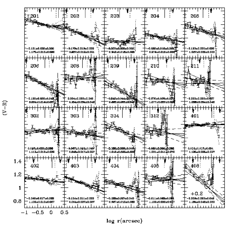
Figure 3: The F555W-F675W color profiles (with statistical errors) and the logarithmic gradient fits of the 20 brightest early-type galaxies of CL0949. Notice that since the colors of N408 are particularly red, we plot the observed colors shifted by -0.2 mag. The shift of 0.2 mag indicated in the figure has to be added to get the real colors of the object. The dotted curved lines show the systematic errors on the colors due to sky subtraction. The straight full lines show the fitted gradients and their statistical errors. The straight dashed lines show their systematic errors. Relevant radial distances are marked on the top x axis of each panel as vertical lines: the location of $R_{e}(675)$ (solid); the minimum and maximum radius used in the fit (dotted); the $0.2R_{e}-2R_{e}$ range (arrows) used in the modeling. Finally, each panel is labeled with the galaxy name, and with the gradient slope (upper row) and zero point (lower row) followed by their statistical and systematic error.

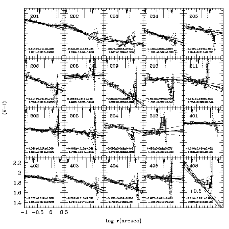
Figure 4: The F555W-F814W color profiles and logarithmic gradient fits of the 20 brightest early-type galaxies of CL0949. Lines and labels as in Fig. 3. The shift to be applied to the colors of N408 is shown as in Fig. 3.

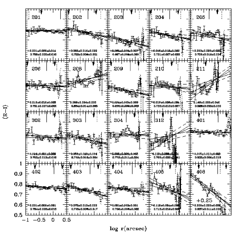
Figure 5: The F675W-F814W color profiles and logarithmic gradient fits of the 20 brightest early-type galaxies of CL0949. Lines and labels as in Fig. 3. The shift to be applied to the colors of N408 is shown as in Fig. 3.

Table 3: The results of the fits to the (V-R) color profiles. Col. 1 gives the galaxy name (see Fig. 1), Col. 2 the fitted logarithmic gradient in mag per radial decade, Col. 3 the statistical error, Col. 4 the systematic error, Col. 5 the fitted color at 0.5 $R_{e}(675)$, Col. 6 the statistical error, Col. 7 the systematic error.

Name	a(V-R)	dast	dasy	Col	dColst	dColsy
201	-0.101	0.023	0.025	1.178	0.015	0.019
202	-0.179	0.019	0.039	1.082	0.016	0.011
203	-0.007	0.028	0.035	0.947	0.027	0.002
204	-0.083	0.018	0.039	1.019	0.015	0.012
205	-0.120	0.035	0.036	1.141	0.031	0.009
206	-0.198	0.023	0.043	1.100	0.019	0.014
208	0.024	0.052	0.049	1.139	0.047	0.012
209	-0.245	0.044	0.048	0.981	0.033	0.018
210	-0.072	0.059	0.050	1.134	0.060	0.005
211	-0.083	0.088	0.057	1.155	0.106	0.012
302	0.026	0.033	0.038	1.099	0.026	0.009
303	-0.067	0.028	0.043	1.082	0.024	0.010
304	-0.155	0.039	0.046	1.144	0.033	0.009
312	-0.058	0.066	0.082	1.125	0.083	0.020
401	0.013	0.015	0.034	1.192	0.009	0.017
402	-0.048	0.017	0.033	1.115	0.011	0.019
403	-0.154	0.011	0.033	1.084	0.009	0.012
404	-0.123	0.027	0.040	1.037	0.019	0.016
405	-0.011	0.053	0.054	1.131	0.055	0.002
408	-0.359	0.063	0.046	1.268	0.046	0.040

Table 4: The results of the fits to the (V-I) color profiles. Columns as in Table 3.

Name	a(V-I)	dast	dasy	Col	dColst	dColsy
201	-0.114	0.011	0.028	1.963	0.007	0.021
202	-0.225	0.016	0.034	1.864	0.013	0.010
203	-0.077	0.041	0.032	1.663	0.039	0.003
204	-0.165	0.015	0.037	1.777	0.012	0.012
205	-0.090	0.024	0.034	1.896	0.022	0.009
206	-0.217	0.031	0.041	1.858	0.026	0.013
208	0.026	0.034	0.046	1.926	0.031	0.011
209	-0.325	0.043	0.045	1.688	0.033	0.017
210	-0.015	0.039	0.046	1.879	0.041	0.005
211	-0.141	0.042	0.052	1.904	0.051	0.010
302	-0.040	0.022	0.038	1.862	0.016	0.008
303	-0.087	0.018	0.042	1.830	0.016	0.010
304	-0.085	0.041	0.043	1.927	0.035	0.008
312	0.032	0.044	0.077	1.797	0.055	0.018
401	-0.008	0.010	0.032	1.991	0.007	0.016
402	-0.077	0.015	0.032	1.881	0.009	0.018
403	-0.207	0.012	0.037	1.835	0.009	0.013
404	-0.182	0.031	0.038	1.783	0.022	0.015
405	-0.037	0.031	0.051	1.917	0.032	0.002
408	-0.616	0.071	0.054	2.241	0.050	0.043

Table 5: The results of the fits to the (R-I) color profiles. Columns as in Table 3.

Name	a(R-I)	dast	dasy	Col	dColst	dColsy
201	-0.001	0.009	0.014	0.788	0.005	0.009
202	-0.055	0.016	0.029	0.782	0.012	0.005
203	-0.069	0.016	0.027	0.718	0.015	0.000
204	-0.049	0.013	0.032	0.757	0.010	0.005
205	-0.050	0.028	0.033	0.751	0.023	0.004
206	-0.012	0.012	0.029	0.758	0.010	0.006
208	0.069	0.024	0.035	0.790	0.020	0.004
209	-0.054	0.015	0.029	0.716	0.011	0.009
210	-0.019	0.026	0.034	0.753	0.025	0.000
211	0.149	0.059	0.042	0.673	0.070	0.013
302	-0.024	0.024	0.029	0.766	0.018	0.003
303	-0.059	0.020	0.034	0.755	0.016	0.003
304	-0.002	0.023	0.035	0.779	0.018	0.002
312	0.113	0.058	0.054	0.664	0.072	0.018
401	-0.005	0.010	0.023	0.804	0.006	0.009
402	-0.021	0.008	0.021	0.769	0.005	0.010
403	-0.072	0.010	0.023	0.747	0.007	0.006
404	-0.031	0.012	0.031	0.751	0.008	0.009
405	-0.112	0.034	0.038	0.808	0.034	0.004
408	-0.208	0.022	0.039	0.999	0.013	0.020

Fig. 6 summarizes the properties of the gradient sample. No correlation is observed between galaxy size and/or galaxy magnitude and gradients. All objects have detected negative gradients in at least one color. For at least half of the sample the gradients are detected with at least $3\sigma$ significance. None of the positive gradients is statistically significant. The systematic errors are on average larger than the statistical ones. Due to the rather large errors, the correlation between the gradients in the different bands is not very strong.

Figure 6: Top-left: the color gradients of the distant sample as a function of $R_{e}(675)$ in arcsec. Open squares refer to the $(V-R)$, crosses to the $(V-I)$ and filled squares to the $(R-I)$ colors. The bars show the statistical errors. Bottom-left: the color gradients of the distant sample as a function of $m_{T}(675)$. The bars show the systematic errors. Top-middle: the cumulative distribution of ratio between the gradient and the statistical error. The solid line refers to the $(V-R)$, the dotted to the $(V-I)$, the dashed to the $(R-I)$ colors. The vertical line shows the $3\sigma$ limit. Bottom-middle: the correlation between statistical and systematic errors. Symbols as above. Top-right: the correlation between the $(V-R)$ and the $(R-I)$ gradients. Statistical errors are shown. Bottom-right: the correlation between the $(V-I)$ and the $(R-I)$ gradients. Statistical errors are shown.

3 The Local Sample

Since the F555W, F675W, F814W bands at $z\approx 0.4$ map approximately the $U$, $B$, $V$ Johnson filters at $z=0$, the direct comparison of our measured color gradients with those derived for local early-type galaxies in the U, B, V bands can give a first idea of their evolution. Therefore, we consider the surface brightness profiles measured by Franx et al. (FIH89 (1989)), Peletier et al. (PDIDC90 (1990)), and Goudfrooij et al. (GHJNDV94 (1994)). Focusing on cluster galaxies our sample consists of 21 objects, for which at least one color gradient is available. Table 6 lists the selected cluster galaxies, their membership, the color gradient, the colors at $R_{e}/2$ and the source of the photometry. For those objects with source of photometry “I”, the $V$ profile was not available. We derived it by interpolation of the B and R profiles using the relation $(B-V)=0.66\times(B-R)-0.03$, which was determined from the SSP models of Maraston (2000) for ages older than 4 Gyr, independently of the metallicities. The errors on the quantities given in Table 6 are systematic and due to the uncertainties in the sky subtraction. The statistical errors are (usually) much smaller. Inspection of Table 6 shows that our local galaxy sample consists of 16 objects in $(U-B)$ and $(U-V)$, and 21 in $(B-V)$. In the following we indicate with DS the distant sample of E galaxies of CL0949 at $z\approx 0.4$ and with LS the local sample of cluster E galaxies from the literature. Figure 7 shows the comparison of the cumulative distributions of the absolute total B band magnitudes of the two samples, having applied 0.4 mag dimming (cf. Ziegler et al. ZSBBGS99 (1999)) to the DS galaxies. The distributions look similar (the Kolmogorov-Smirnov probability is 0.28), although the LS suffers from incompleteness at magnitudes fainter than $\approx$ -21. On the whole, the comparison between the two samples is fair.

Figure 7: Cumulative distributions of the B-band absolute magnitudes of the z=0 (solid) and $z\approx 0.4$ (dotted) samples.

Table 6: The color gradients of the Local Sample. Column 1 gives the galaxy name, Col. 2 the galaxy cluster (F for Fornax, V for Virgo, C for Coma), Col. 3 the U-B logarithmic gradient, Col. 4 its error, Col. 5 the U-B color at $R_{e}/2$, Col. 6 its error, Col. 7 the source, Col. 8 the U-V logarithmic gradient, Col. 9 its error, Col. 10 the U-V color at $R_{e}/2$, Col. 11 its error, Col. 12 the source, Col. 13 the B-V logarithmic gradient, Col. 14 its error, Col. 15 the B-V color at $R_{e}/2$, Col. 16 its error, Col. 17 the source. The source codes are: F for Franx et al. FIH89 (1989), G for Goudfrooij et al. GHJNDV94 (1994), P for Peletier et al. PDIDC90 (1990), I indicates that the V profile was obtained interpolating the B and R profiles (see text). Errors are due to sky subtraction and therefore systematic.

Galaxy	Cl	a(U-B)	da	U-B	dCol	S	a(U-V)	da	U-V	dCol	S	a(B-V)	da	B-V	dCol	S
A 496	-	-0.05	0.10	0.57	0.01	P	-0.28	0.11	1.45	0.12	I	-0.10	0.02	0.94	0.03	I
IC 1101	-	-0.05	0.10	0.69	0.01	P	-0.09	0.12	1.71	0.15	I	-0.06	0.03	0.97	0.04	I
NGC 1379	F	-0.06	0.18	0.40	0.09	F	-0.02	0.28	1.35	0.03	I	-0.05	0.04	0.92	0.02	I
NGC 1399	F	-0.08	0.15	0.55	0.07	F	-0.15	0.12	1.52	0.06	F+G	-0.07	0.01	0.97	0.02	G
NGC 1404	F	-0.07	0.04	0.57	0.01	F	-0.08	0.03	1.53	0.01	F+G	-0.01	0.01	0.96	0.01	G
NGC 1427	F	-	-	-	-	-	-	-	-	-	-	-0.05	0.01	0.89	0.01	G
NGC 4365	V	-	-	-	-	-	-	-	-	-	-	-0.04	0.01	0.97	0.01	G
NGC 4374	V	-0.17	0.02	0.54	0.01	P	-0.22	0.04	1.57	0.02	I	-0.04	0.01	1.02	0.01	I
NGC 4387	V	-0.01	0.02	0.49	0.01	P	0.01	0.08	1.54	0.02	I	-0.02	0.02	1.05	0.01	I
NGC 4406	V	-0.15	0.02	0.52	0.01	P	-0.16	0.03	1.52	0.02	I	-0.02	0.01	1.00	0.01	I
NGC 4472	V	-0.15	0.03	0.55	0.01	P	-0.18	0.05	1.58	0.03	I	-0.03	0.01	1.05	0.01	I
NGC 4478	V	-0.12	0.04	0.52	0.01	P	-0.14	0.07	1.52	0.02	I	-0.03	0.02	0.99	0.01	I
NGC 4486	V	-0.23	0.04	0.41	0.01	P	-0.27	0.03	1.37	0.01	P+G	-0.04	0.01	0.96	0.01	G
NGC 4564	V	-	-	-	-	-	-	-	-	-	-	-0.12	0.01	0.93	0.01	G
NGC 4621	V	-	-	-	-	-	-	-	-	-	-	-0.03	0.01	0.92	0.01	G
NGC 4636	V	-0.22	0.04	0.46	0.01	P	-0.27	0.07	1.45	0.05	I	-0.05	0.02	0.99	0.01	I
NGC 4649	V	-0.15	0.04	0.65	0.01	P	-0.18	0.06	1.69	0.03	I	-0.04	0.01	1.04	0.01	I
NGC 4660	V	-	-	-	-	-	-	-	-	-	-	-0.05	0.01	0.98	0.01	G
NGC 4874	C	-0.07	0.06	0.55	0.01	P	-0.20	0.05	1.50	0.05	I	-0.10	0.02	0.97	0.01	I
NGC 4889	C	-0.08	0.04	0.72	0.01	P	-0.11	0.09	1.65	0.04	I	-0.10	0.03	0.95	0.02	I
NGC 6086	-	-0.15	0.04	0.62	0.01	P	-0.17	0.14	1.58	0.06	I	-0.03	0.03	0.96	0.01	I

Fig. 8 compares the cumulative distributions of the measured gradients for the LS and the DS samples. The distributions appear rather similar, suggesting little evolution. In particular, the median values of the $(U-B)$, $(U-V)$ and $(B-V)$ gradients of the LS galaxies are -0.12, -0.17 and -0.06 mag/dex per decade respectively. These are close to, but somewhat steeper than the median values of the $(V-R)$, $(V-I)$, and $(R-I)$ gradients of the DS galaxies, that are respectively -0.09, -0.08, -0.03 mag/dex per decade. A Kolmogorov-Smirnov (KS) test shows that only the (B-V), (R-I) pair of distribution is marginally different.

In the following we will investigate quantitatively the evolutions of color gradients under different assumptions for their origin and compare the models to the observed distributions.

Figure 8: Cumulative distributions of color gradients of the z=0 (solid) and $z\approx 0.4$ (dotted) samples. The left, central and right panels show respectively the $(U-B)$, $(U-V)$ and $(B-V)$ gradients of the LS, to be compared to the $(V-R)$, $(V-I)$ and $(R-I)$ gradients of the DS. Each panel is labeled with the results of the KS tests applied to the corresponding pairs of distributions.

4 The Models

4.1 The Basic Tool: Simple Stellar Populations

Our modeling is based on the assumption that the light-averaged stellar population in the Es between $z\approx 0.4$ and $z=0$ can be described by Simple Stellar Populations (SSP), i.e. coeval and chemically homogeneous assemblies of single stars. The SSP models for this work are computed with the evolutionary synthesis code described in Maraston (Ma98 (1998)), in which the Fuel Consumption theorem (Renzini & Buzzoni RB86 (1986)) is used to evaluate the energetics of Post Main Sequence stars. The input stellar tracks for the SSP models used here are from Cassisi (private communication; see also Bono et al. bono97 (1997)), covering the metallicity range ${\rm[Fe/H]}=[-1.35\div 0.35]$, with helium-enrichment parameter ${\rm\Delta Y/\Delta Z}$=2.5. The amount of mass loss along the Red Giant branch (RGB) is parametrized a’ la Reimers (R75 (1975)), with the efficiency $\eta$=$0.33$ as calibrated by Fusi Pecci & Renzini (FPR76 (1976)). The mass loss prescriptions affect the evolutionary mass on the horizontal branch (HB), leading to warmer HBs as the mass loss increases. We adopt Salpeter IMF ($\Psi(m)=A{m}^{-(1+x)}$, $x$=1.35) down to a lower mass limit of 0.1 M_⊙. For plausible variation of the IMF slope, the optical colors of SSPs are virtually unchanged (e.g. Maraston Ma98 (1998)). The evolutionary synthesis code has been updated for the computation of the SSP Spectral Energy Distributions (SEDs), as a function of $t$ and [Fe/H]. We adopted the spectral library of Lejeune, Cuisinier and Buser (LCB98 (1998)) to describe the stellar spectra as functions of gravity, temperature and metallicity. A redshifted grid of SSP model SEDs has also been computed to interpret the colors of the DS galaxies. We have applied the same redshift $z=0.3775$ to all the models. This is the average value of the $z$ distribution of the DS sample, having assigned to the galaxies without redshift determination, the average redshift value of the objects with a measured redshift. The uncertainties introduced by a $\approx 0.03$ variation in redshift are of the same order as the statistical errors. Model SEDs have been convolved with the $UBVRI$ Johnson-Cousins filter functions (Buser B78 (1978), Bessel B79 (1979)) to yield synthetic magnitudes. The applied zero points are ($U$,$B$,$V$,$R$,$I$)=(0.02, 0.02, 0.03, 0.0039, 0.0035) for the Vega model atmosphere of Kurucz (K79 (1979)) with ($T_{e}$, g, [Fe/H])=(9400, 3.9, -0.5). This ensures consistency with our HST photometry (Holtzman et al. 1995). We refer to Maraston (Ma99 (2000)) for more details.

Figures 9 and 10 summarize the properties of the models relevant to our case. Fig. 9 shows the $(U-B)$, $(U-V)$ and $(B-V)$ colors of the rest-frame SSP models, together with their derivatives with respect to age and metallicity (given as [Fe/H]). Derivatives are computed as finite differences on the grid and assigned to the midpoints in age and metallicity.

In general, optical colors become redder with increasing age and/or increasing metallicity. In our models, there are two exceptions to this trend, both at low metallicities. The [Fe/H] = -1.35 models become bluer in $U-B$ as they age from $\sim$ 3 to $\sim$ 5 Gyr. This is due to the properties of the $U-B$ stellar colors for $T_{\rm e}\sim$ 8500-7500 K (see e.g. Castelli C99 (1999)) typical of turnoff stars in this age range. At higher metallicities this effect does not appear, because when the turnoff stars have temperatures in this range, their contribution to the total light is less important due to the presence of AGB stars (Maraston Ma99 (2000)).

At old ages, the same set of models become bluer and bluer in $B-V$ from $\sim$ 12 Gyr onward, reflecting warmer and warmer HBs. With $\eta=0.33$, this effect sets in for [Fe/H]$\la-0.5$. It disappears when no mass loss is applied (Maraston Ma99 (2000); see also Chiosi et al. CBB88 (1988)). The time derivative of colors shows a noisy behavior due to the discrete modeling. However, a general trend can be appreciated, with the derivative initially decreasing and leveling off at $\sim$ 0.01 – 0.04 mag/Gyr for ages older than $\sim$ 7 Gyr. The time derivatives appear almost independent on metallicity for $Z\geq$ 0.5 Z_⊙, while the lowest $Z$ set of models behave differently due to the two effects described above.

The derivatives of colors with respect to metallicity show a different trend with age, with colors generally becoming more and more sensitive to [Fe/H] as the SSPs get older. It is worth noticing that the plotted curves are color variations per metallicity decade. The dependence on $Z$ is quite different, with low metallicity model colors much more sensitive to $Z$ variations than the high $Z$ ones. We preferred to plot the derivatives with respect to [Fe/H] because these are the actual tools used in our simulations. We also point out that in our models the helium abundance varies in lock-steps with $Z$. This influences the temporal behavior of the SSP colors and of their derivatives, especially at high metallicity.

Figure 11 compares our models (shown down to younger ages for the purpose) to the ones of Vazdekis et al. (Vetal96 (1996)), Bruzual & Charlot (BC99 (1996)) and Worthey (W94 (1994)) as a function of metallicity and age (see Maraston Ma98 (1998) for a comparison to the models of Tantalo et al. Tetal96 (1996) at solar metallicity). On the whole, the agreement between all the models in the $(B-V)$ color is good. The variations between the models are of the same order of the uncertainties in the observed colors. Our SSP optical colors compare remarkably well with Vazdekis et al. (Vetal96 (1996)). Larger differences between the models are observed in the $(U-B)$. Bruzual & Charlot (BC99 (1996)) models tend to have systematically redder $(U-B)$. Worthey (W94 (1994)) models produce instead systematically bluer $(U-B)$ (and $(U-V)$) colors at a given $(B-V)$. A thorough investigation of these discrepancies will be presented in Maraston (Ma99 (2000)). The age (at fixed metallicity) or metallicity (at fixed age) differences inferred using the different models between the central and outer parts of the galaxies (the galaxy NGC 1399 is shown as an example) are consistent within the errors. The results on the origin of the color gradients presented here also depend on the derivatives of the colors with respect to age and metallicity. This dependence is difficult to estimate quantitatively because of the coarseness of the grid of the other sets of models, and of the unavailability of their entire SEDs. The close similarity of our models to the Vazdekis is reassuring.

Similar to Fig. 9, Fig. 10 shows the properties of the redshifted SSP SEDs in the $V$, $R$ and $I$ bands. Broadly speaking, the $(V-R)$, $(V-I)$ and $(R-I)$ colors trends with age resemble those of the $(U-B)$, $(U-V)$ and $(B-V)$ colors. Some differences are present, as a result of the different effective wavelengths and sensitivity curves of the corresponding pairs of filters. In particular we notice that the time derivative of the $(V-I)$ color is approximately a factor of 2 smaller than that of the $(U-V)$ color, reminiscent of Fig. 8. Thus we expect that the $(U-V)$ colors of nearby galaxies are more sensitive to age gradients than the $(V-I)$ colors of distant objects.

Simple inspection of Figs. 9 and 10 already allows us to define the framework for the interpretation of color gradients in ellipticals. The filled and open dots show the 0.2 and 2 $R_{e}$ colors of the LS and DS galaxies. It is clear that the range of ages and metallicities considered here is adequate to model the observed colors both as a pure age sequence (at a fixed metallicity) or as a pure metallicity sequence (at a fixed age).

Turning now to the gradients’ evolution, we start considering that the LS galaxies all (with one exception) have negative gradients, with colors being redder in the central regions. Thus, if they are caused by age gradients only, centers must be older than the outer parts ($\approx 5$ Gyr per radial decade). In addition, if the present age of the Es centers is large enough ($\approx 15$ Gyr), we expect the age derivatives of the colors to stay approximately constant for look-back times up to $\approx 7$ Gyr, and therefore to measure color gradients in the DS of approximately the same size in $(V-R)$ and $(R-I)$, and twice as small in $(V-I)$.

In contrast, if color gradients are caused by metallicity gradients only, the centers of local Es must be more metal rich than the outer parts ($\approx 1.6$ more metal rich per radial decade). In addition, given the increase with age of the metallicity derivatives of the colors, we expect the color gradients of the DS to be flatter than those of the LS. This effect should be less prominent if the centers of ellipticals are old.

As noted in Sect. 2, some of the gradients measured in CL0949 Es are positive. In Sect. 6.3 we shall argue that these are caused by measurement errors, with an underlying distribution of intrinsically negative gradients. Here we note that a change in sign with time of the color time derivative of SSP models is possible only at low metallicities and/or low ages. Color gradients caused by metallicity cannot change sign with time following passive evolution.

Figure 9: The colors, time and [Fe/H] derivatives of the rest-frame SSP models in the U, B and V bands. The different line type of the color and time derivative rows refer to the metallicities indicated in the top-left plot. The line types and their corresponding metallicities (midpoints of the above) of the [Fe/H] derivative are given in the bottom panel of the central figure. The filled dots show the 0.2 $R_{e}$ colors of the LS galaxies with ages assigned on the solar metallicity line. The open dots show their 2 $R_{e}$ colors at the (arbitrary) age of 14 Gyr.

Figure 10: The colors, time and [Fe/H] derivatives of the redshifted SSP models in the $V,\leavevmode\nobreak\ R,\leavevmode\nobreak\ I$ bands. The different line type of the color and time derivative rows refer to the metallicities indicated in the top-middle plot. The line types and their corresponding metallicities (midpoints of the above) of the [Fe/H] derivative are given in the bottom-left plot. The vertical lines show the age (5.47 and 10.47 Gyr) of galaxies at z=0.3775 that today are 10 and 15 Gyr old, respectively. The filled dots show the 0.2 $R_{e}$ colors of DS galaxies with ages assigned on the solar metallicity line. The open dots show their 2 $R_{e}$ colors at the (arbitrary) age of 14 Gyr.

Figure 11: The $(U-B)$ (top) and $(B-V)$ rest-frame color time evolution of our model (full lines), Vazdekis et al. (Vetal96 (1996), dotted lines), Worthey (W94 (1994), short-dashed lines), Bruzual & Charlot (BC99 (1996), long-dashed lines) as a function of age (for three metallicities) and metallicity (15 Gyr age for our models and Bruzual & Charlot, 17 Gyr for Vazdekis and Worthey’s models). The error bars show the allowed range of the inner (at $0.2R_{e}$) colors of the LS galaxies derived from the gradient fits. The filled circles and squares show the inner and outer ($2R_{e}$) colors, respectively, of the galaxy NGC 1399.

4.2 Modeling the Evolution of Color Gradients

The detailed modeling of the color gradients evolution of each galaxy involves a number of steps. As a starting point, a cosmological model should be chosen to fix the look-back time at $z\approx 0.4$. Here we adopt ${\rm H_{o}}$=65 ${\rm Km\cdot s^{-1}\cdot Mpc^{-1}}$ and $\rm{\Omega_{m}}$=0.2, with ${\rm{\Lambda}}=0.8$. The age of the Universe is $\approx$ 16.18 Gyr and $t_{\rm lb}=4.53$ Gyr at $z$=0.3775. The choice of the cosmological parameters is not crucial to model color gradients, but a much younger universe (for example, 10 Gyr) would strongly disfavor the age hypothesis for the origin of color gradients (see below). In addition, the look-back time has an influence on the exact value of the predicted colors. As we will show later, the optimal agreement between the observed color distributions in the LS and the DS samples is achieved for larger look-back times, i.e., $t_{\rm lb}\approx 8$ Gyr.

Inspection of Figs. 3-5 shows that the color gradients of the DS galaxies are measured in the radial range $0.2-2\leavevmode\nobreak\ R_{e}$. The same applies to most of the local galaxies. Therefore, we choose this radial decade to model the gradients. A more innerly defined decade (i.e., $0.1-1\leavevmode\nobreak\ R_{e}$) suffers of insufficient resolution for the more distant sample. A more outerly defined decade (i.e., $0.3-3\leavevmode\nobreak\ R_{e}$) is poorly investigated in the local sample. Thus, we analyse a given color gradient by examining the colors at the $0.2\leavevmode\nobreak\ R_{e}$ (hereafter, the central region) and $2\leavevmode\nobreak\ R_{e}$ (hereafter, the outer region) isophotes, as derived from the values listed in the Table 3-6.

We need now to choose representative SSP models for the inner and outer regions. Due to the age-metallicity degeneracy, one parameter has to be fixed to derive the other from the observed colors. For the central stellar populations we consider two options: 1) Case m, in which all the galaxy centers have the same age and the colors are used to infer their metallicities; 2) Case a, in which all the galaxy centers have the same metallicity, and their colors are used to infer their ages. In Case m we explore two possible current ages: 10 and 15 Gyr; in Case a we assign solar metallicity to all the galaxy centers. A smaller metallicity (i.e., half-solar) would imply implausibly large (larger than the age of the Universe) ages for the galaxies (see Figs. 9 and 10). The canonical interpretation of the Color-Magnitude relation of cluster early type galaxies is consistent with Case m (e.g. Arimoto & Yoshii AY86 (1986), Kodama & Arimoto KA97 (1997)); Case a is nevertheless worth exploring.

As for the gradients, we consider the two extreme possibilities that they are driven by pure age (A) or pure metallicity (M) gradients. Thus we have four scenarios in which we model the evolution of the color gradients:

• age drives the color gradients. Central and outer SSPs have solar $Z$ and colors reflect their ages. The gradients are expected to steepen with look-back time if the centers are young; to remain nearly constant if they are old enough.

• age drives the color gradients. The central SSPs of local Es are 10 or 15 Gyr old (mA10 and mA15); the outer SSPs have the same metallicity as the central ones, but different ages. The gradients’ evolution is expected to be similar to case aA.

• metallicity drives the color gradients. Central SSPs have solar $Z$; the outer SSPs have the same age as the centers, but different metallicities. Color gradients are expected to flatten with look-back time.

• metallicity drives the color gradients. The central and outer SSPs of local Es are coeval and 10 or 15 Gyr old (mM10 and mM15), and the colors reflect their metallicities. The gradients’ evolution is expected to be similar to case aM.

To summarize, we model the evolution of the color gradients of each galaxy in the LS in the four scenarios by:

• fixing the age and metallicity of the central and outer SSPs according to the specific option (aA,aM,mA and mM);

• rejuvenating the SSPs by the adopted look-back time (4.53 Gyr);

• computing the color gradients of the rejuvenated and redshifted SSPs in the $V,\leavevmode\nobreak\ R$ and $I$ bands.

For consistency, we also perform the reverse experiment and compute the predicted $U,B,V$ color gradients of the CL0949 galaxies after $t_{LB}$ (i.e., 4.53 Gyr) of passive evolution. We tested that the results we are going to discuss remain the same within the errors if the whole color profiles are modeled at each radial distance, and a logarithmic gradient is fit to the predicted profiles at z=0.

5 Ages and Metallicities of the Galaxies in the Four Scenarios

We consider now the applicability of the four scenarios to our local and distant galaxy samples. Indeed, the ages or metallicities derived from the three colors available should agree within the measurement errors. The distribution of ages derived for cases aA, aM and mA for the LS and the DS galaxies should be similar, given the look back time. The distributions of metallicities derived for cases aM, mA and mM should also be similar.

5.1 Age gradients: the aA Case

Figures 12 and 13 show the ages assigned to the center (0.2 $R_{e}$) and the outer isophotes (2 $R_{e}$) of the local and distant galaxies, having assumed solar metallicity for both samples in both regions. The ages derived from different colors are in agreement (within the rather large statistical errors), better for the DS objects. We note that the LS objects appear in the plot only when the specific pair of colors is available. However, the average ages and rms indicated in the plots are those obtained considering all the objects with the specified color available. On the average, the centers of LS galaxies appear $\sim$ 12 Gyr old, while the peripheries are $\sim$ 7 Gyr old. The DS galaxies appear $\sim$ 4 Gyr old in the center, $\sim$ 2.5 Gyr old in the peripheries. Thus, the consistency of the aA hypothesis is rather questionable, both because the average age difference between the centers of the two samples is larger than our adopted look-back time, and because the age gradients implied under this scenario are much smaller for the DS sample than for the LS one. In addition, the colors of some local galaxies require a present age younger than 4.5 Gyr or an age older than the age of the universe in our chosen cosmology. In other words, only a subsample of the LS galaxies could be the passively evolved descendants of the CL0949 objects. This is partly a consequence of forcing a solar $Z$ for all the considered SSPs.

Figure 12: Ages assigned to the center (0.2 $R_{e}$) and the outer isophotes (2 $R_{e}$) of the local galaxies, assuming that they have solar metallicity. The given mean age and rms are derived using all the galaxies available in a given filter. The cross shows the mean of the measurement errors.

Figure 13: Ages assigned to the center (0.2 $R_{e}$) and the outer isophotes (2 $R_{e}$) of the distant galaxies, assuming that they have solar metallicity. Labels and crosses as in Fig. 12

5.2 Metallicity gradients: the mM Case

Figures 14 and 15 show the metallicities assigned to the center (0.2 $R_{e}$) and the outer isophotes (2 $R_{e}$) of the local and distant galaxies, assuming a present day age of 15 Gyr for the LS objects. At $z=0$ the metallicities derived from the three colors agree well. Local galaxies appear to be slightly subsolar at their centers if 15 Gyr old, solar if 10 Gyr old. The central SSPs of the DS objects require only half solar metallicity, if the look-back time is 4.53 Gyr, but with t${}_{\rm lb}\approx$ 8 Gyr the central $Z$ is larger by 0.15 dex. This discrepancy is the same present in the aA case: for our adopted look-back time the observed central colors of the DS objects are too blue (those of the LS are too red) when compared to passively evolving models. The metallicity gradients are $\approx$ 0.2 dex for both DS and LS, indicating that metallicity driven color gradients are a viable interpretation (see Sect. 6). However, we notice that the DS galaxies span a wider range in metallicity gradients, compared to LS objects. This indicates a slight inconsistency also for the mM scenario, but see Sect. 6.3 for a possible way out.

Figure 14: Metallicities assigned to the center (0.2 $R_{e}$) and the outer isophotes (2 $R_{e}$) of the local galaxies, assuming that their age is 15 Gyr. The given mean metallicity and rms are derived using all the galaxies available in a given filter. The cross shows the mean of the measurement errors.

Figure 15: Metallicities assigned to the center (0.2 $R_{e}$) and the outer isophotes (2 $R_{e}$) of the distant galaxies, assuming that their age is 10.47 Gyr. Labels and crosses as in Fig. 14.

5.3 The aM and mA Cases

The aM case is always applicable: since the central ages derived in 5.1 are $\approx 12$ Gyr on the average, and the central metallicities are supposed to be solar, the other colors for both DS and LS galaxies can be reproduced consistently in all filters by decreasing the metallicity by 0.2 dex.

The applicability of the mA scenario strongly depends on the assumed central age. When 10 Gyr is adopted for the centers of LS galaxies, a substantial number of objects appear to have outer SSPs younger than our adopted look-back time. In addition, the average age of the outer regions of the DS galaxies is $\approx$ 3 Gyr, too old to evolve into the LS galaxies. The situation is different if the central age of local galaxies is fixed to 15 Gyr. The average outer age of the LS is $\approx$ 10 Gyr in this case, with only a few objects younger than our adopted look-back time. The peripheries of the DS galaxies appear $\approx$ 6 Gyr old on the average, which is consistent with the average age of the LS.

To summarize, the metallicity driven color gradients hypothesis is always applicable, while the age hypothesis holds only if local galaxies are old ($\sim$ 15 Gyr). This reflects the fact that a small metallicity variation is required to explain the observed color gradients, while a large age gradient (of $\sim$ 5 Gyr) is needed to fit the color gradients of the LS objects. With a 4.5 Gyr look-back time, a substantial number of LS galaxies do not have their corresponding object in the DS.

6 Results

In this section we present the results of the detailed modeling of the evolution of the central colors and color gradients under the four scenarios, according to the procedure outlined in Sect. 4.2. We will compare the model predictions to the data by considering the cumulative distribution functions of the color gradients and applying Kolmogorov-Smirnov tests to the pairs of correspondent theoretical and observational distributions. In particular, the redshifted $V,\leavevmode\nobreak\ R,\leavevmode\nobreak\ I$ colors of rejuvenated LS galaxies will be compared to those of CL0949 objects; the $U,\leavevmode\nobreak\ B,\leavevmode\nobreak\ V$ colors of passively evolved DS galaxies will be compared to the $U,\leavevmode\nobreak\ B,\leavevmode\nobreak\ V$ colors of local ellipticals. As discussed above, the colors of some LS galaxies are so blue that ages shorter than $t_{LB}$ would be required. In these cases the object “drops out” of the sample by getting an assigned (blue) color of -1. For some choices of age or metallicity the colors are outside our grid of models. In these cases we assign the minimum (-1.35) or maximum (0.35) metallicities, and 30 Myr of age (the smallest age of the grid), if the extrapolated age is smaller than 0, or 15 Gyr, if larger ages are extrapolated.

6.1 The distributions of central colors

Fig. 16 compares the cumulative distributions of observed and simulated central colors of local and distant galaxies. The Kolmogorov-Smirnov probability KS that the observed and simulated data are drawn from the same underlying distribution are always smaller or equal than 0.001. None of the simulated central color distributions appear compatible with the observed ones. This result is confirmed using the Wilcoxon test. The simulated centers of the DS objects appear too blue (by $\approx 0.04$ mag in $B-V$) when compared to the local ones, and, vice versa, the centers of local galaxies appear too red ($\approx 0.03$ mag in R-I) when compared to the CL0949 galaxies. The differences are more pronounced in the $(U-B)$ and $(V-R)$ and $(U-V)$ and $(V-I)$ pairs. Measurement errors alone seem insufficient to explain the difference between these pairs (see 6.3), while the $(B-V)$ and $(R-I)$ colors might not differ significantly in a statistically sense. The uncertainties in the galaxy redshifts and in the calibration to the Johnson-Cousins system (see Holtzmann et al. HBCHTWW95 (1995)), combined with the notoriously difficult photometric calibration of the U band probably suffice to explain our findings. In any case, we tested that the conclusions concerning the origin of color gradients are not affected by this possible inconsistency of the central colors. The distributions of gradients shown in Fig. 17 are hardly changed when the look-back time is increased from 4.53 to 8 Gyr.

Assuming that the color differences are real, they can be explained using a larger look-back time. For example, $t_{LB}=8$ Gyr (obtained with the same cosmology and a rather extreme low value of the Hubble constant, $H_{0}=37$) gives reasonable KS probabilities (5-80% for the different colors and models). The result might also point to recent, minor episodes of star formation in the distant galaxies (Poggianti et al. Pog98 (1998), Couch et al. Cou98 (1998)).

Figure 16: The cumulative distributions of observed (solid line) and simulated (for $t_{LB}=4.53$ Gyr) central colors of z=0 (top panels) and $z\approx 0.4$ (bottom panels) galaxies. The dotted lines show Case a, the short- and long-dashed line the Case m for present-day central ages of 10 and 15 Gyr. The Kolmogorov-Smirnov probabilities that the observed and simulated data are drawn from the same underlying distribution are always smaller or equal than 0.001.

6.2 The distributions of color gradients

Fig. 17 compares the cumulative distributions of the observed and simulated color gradients. The Kolmogorov-Smirnov probabilities that the observed and simulated data are drawn from the same underlying distribution are given in Table 7.

The aA Case is clearly ruled out. The very small differences between the central and outer ages required at $z\approx 0.4$ (see Fig. 13) evolve into too shallow gradients at z=0. Along the same line, the 5 Gyr age difference inferred at z=0 (see Fig. 12) produces too steep gradients at $z\approx 0.4$, because the color time derivatives increase for decreasing age (see Fig. 9 and discussion in Sect. 4.1).

The mM case is viable for both the assumed present-day central ages of 10 and 15 Gyr. The t-test confirms that the means of the observed and simulated distributions in all colors at both z=0 and $z\approx 0.4$ are statistically identical. The f-test on the rms of the distributions confirms the slightly lower KS probabilities obtained for the $B-V$ gradients for z=0 and for the $(R-I)$ for z$\approx 0.4$. As discussed in Sect. 4.1, all (except one) local gradients are negative, while some positive gradients are observed at $z\approx 0.4$. This makes the observed widths of the $z\approx 0.4$ gradient distributions larger than the simulated ones. Errors might partly explain this effect (see discussion in Sect. 6.3). Indeed, the widths of the distributions are somewhat dissimilar, with the DS presenting a tail of steep gradients with no counterpart in the simulated LS. Since the metallicity color derivatives decrease with decreasing age, the evolution leads to shallower (not steeper) gradients. The same considerations apply to the aM Case, which provides also an acceptable model of color gradients.

The mA Case does not offer a perfect clear-cut solution. One can clearly exclude the case of central present-day young ages (10 Gyr), since the resulting outer ages at z=0 are either younger than the assumed $t_{LB}$, or so young to correspond to a very steep rejuvenated color gradient. The outer colors of the distant galaxies require such large ages that too shallow gradients are produced at z=0. In contrast, present day central ages of 15 Gyr still make the age hypothesis a possible explanation for color gradients. In this case, the outer ages (some $\approx 5$ Gyr smaller than the central ones) required to match the colors of the z=0 galaxies are large enough (see Sect. 5.3) to produce mild gradients at $z\approx 0.4$, even if a tail of too steep gradients is produced, which is not observed in the data. Similarly, only a small fraction ($\approx 10-20$%) of the distant galaxies cannot be matched in their outer colors by this mechanism. The remaining objects are assigned outer ages that produce reasonable gradients locally.

Figure 17: The cumulative distributions of observed and simulated color gradients of z=0 (top panels) and $z\approx 0.4$ (bottom panels) galaxies. In each of the plots the thick solid line shows the observed distributions. Two rows of plots are shown for the local and distant case. The top row refers to the age-driven color gradients. Here the dotted lines show the aA case, the short-dashed lines the mA10 case, the long-dashed lines the mA15 case. The bottom row refers to the metallicity-driven color gradients. Here the dotted lines show the aM case, the short-dashed lines the mM10 case, the long-dashed lines the mM15 case. The Kolmogorov-Smirnov probabilities that the observed and simulated data are drawn from the same underlying distribution are given in Table 7.

Table 7: The Kolmogorov-Smirnov probabilities of the color gradient distributions. Col. 1 gives the examined Case, Cols.2-5 the KS probabilities for the $(U-B)$, $(U-V)$, $(B-V)$ color gradients at $z=0$, Cols. 6-7 for the $(V-R)$, $(V-I)$, $(R-I)$ at $z\approx 0.4$.

Case	KSU-B	KSU-V	KSB-V	KSV-R	KSV-I	KSR-I
aA	7.5e-05	4.4e-06	2.9e-07	0.05	0.013	0.002
mM10	0.79	0.50	0.18	0.62	0.50	0.18
mM15	0.67	0.51	0.09	0.17	0.29	0.22
aM	0.37	0.15	0.20	0.83	0.50	0.32
mA10	0.016	0.004	0.08	0.009	0.0002	2.7e-05
mA15	0.83	0.50	0.01	0.62	0.87	0.18

6.3 The influence of errors

In the previous sections we pointed out that some of the problems recognized in the modeling (the difference in the median central colors of the LS and DS samples, the presence of positive gradients at $z\approx 0.4$, the differences in the observed and predicted width of the gradient distributions) might be explained taking into account the observational errors. Errors are dominated by systematics for the LS galaxies, and have both a statistical and a systematic component for the DS. They affect both the observed and the predicted distributions. We estimate the effect of statistical errors on the observed distributions by bootstrapping the measured colors or color gradients with their statistical errors, assumed to be gaussianly distributed. The estimation of the effect on the predicted color and color gradient distributions requires the choice of a model. For simplicity, we focus on the mM Case with present-day age of 10 Gyr. We bootstrap the measured colors at 0.2 and 2 $R_{e}$ with their statistical errors at $z\approx 0.4$, assumed to be gaussianly distributed. We compute the metallicities implied by the SSP models, predict the expected colors at z=0, and derive the color gradients and their cumulative distributions. Figs. 18 and 19 show the result of 30 such bootstraps. The typical width of the obtained measured and predicted color distribution clouds is $\approx 0.02$ mag. As discussed in Sect. 2, the statistical errors dominate over the systematic effects. The typical width of the obtained measured and predicted distributions clouds of the color gradients is $\approx 0.02-0.04$ mag/dex. In this case the systematic effects bracket the statistical variations.

Figure 18: The influence of statistical and systematic errors on the cumulative distributions of the observed and predicted central colors for the LS (upper) and the DS (lower) galaxies. For the DS galaxies and for each color we show 30 distributions (dotted lines) obtained by bootstrapping the measured colors and modeling their evolution (see text for explanation). The thick lines show the measured distributions. The dashed thick lines show the effects of systematic errors. For the LS galaxies we show the measured and evolved distributions taking into account the systematic errors (lines with crosses).

Figure 19: The influence of statistical and systematic errors on the cumulative distributions of the observed and predicted color gradients for the LS (upper) and the DS (lower) galaxies. For the DS galaxies and for each color we show 30 distributions (dotted lines) obtained by bootstrapping the measured colors and modeling their evolution (see text for explanation). The thick lines show the measured distributions. The dashed thick lines show the effects of systematic errors. For the LS galaxies we show the measured and evolved distributions taking into account the systematic errors (lines with crosses).

Fig. 18 shows that measurement errors alone are insufficient to explain the difference in central color between the LS and DS samples, because the simulated and observed distributions at both z=0 and $z\approx 0.4$ are separated even when errors on both sides are considered. A larger look-back time (8 Gyr) produces a good overlap.

The inspection of Figure 19 shows first that the results described in Sect. 6.2 are robust against the errors. Cases aA and mA with a central present age of 10 Gyr are ruled out with high significance because the large tail of steep negative gradients that they produce at $z\approx 0.4$ is not present in any of the distributions with errors. As a second remark, errors help explaining the discrepancies between the observed and modeled distributions. Complete overlap at both z=0 and $z\approx 0.4$ is achieved between the observed and modeled distributions of the U-B and $V-R$ gradients. The agreement for the $U-V$ and $V-I$ gradient distributions is improved, with most of the differences in the widths accounted by the errors. The 10% tail of distant galaxies with the largest positive R-I gradients (objects 211 and 312) cannot be explained by the observational errors. However, the two galaxies are the smallest of the sample and it can be argued that their gradients are not well determined (see Sect. 2). Therefore, we conclude that the mM, aM, and, to less extent, mA15 cases provide a satisfactory description of the color gradients of (bright) cluster ellipticals at z=0 and $z\approx 0.4$ following passive evolution.

6.4 The role of dust

Wise & Silva (WS96 (1996)) examined the possibility that color gradients in elliptical galaxies are caused entirely by dust effects. They fit the color profiles of the LS galaxies considered here adopting different radial distributions and total mass of the dust component. Their best fitting models are characterized by a distributions $\propto r^{-1}$ and dust masses much higher than those directly determined from the IRAS data. The ratios of these masses are in the range 3.6-307, only NGC 1399 having ratio of order unity. Therefore we are confident that the radial variation of the stellar populations plays a major role in driving the color gradients. Nevertheless, part of the gradient may be due to dust. We have thus tested the hypothesis that 50% of the color gradients observed are caused by dust, to verify how robust our conclusions of Sect. 6.2 are. We reduce the gradients by a factor 2 by making the 0.2 $R_{e}$ colors bluer and leaving the 2 $R_{e}$ as measured. As a consequence, for Case a we require central mean ages smaller by $\approx 2$ Gyr at z=0 but only shorter by $\approx 0.4$ Gyr at $z\approx 0.4$. For Case m we require central mean metallicities smaller by $\approx 0.1$ dex. This does not modify much our conclusions about the viability of the different mechanisms examined in Sect. 6.2. Case aA remains ruled out with high confidence. A metallicity change (Cases mM and aM) of $\approx 0.1$ dex per radial decade is enough to match both local and distant gradient distributions. The Case mA with 15 Gyr central ages and $\approx 2.5$ Gyr younger peripheries allows a consistent model of all local and distant objects. The Case mA with 10 Gyr central ages is less unprobable than before, but still not acceptable.

These findings can be used to estimate the viability of mixed scenarios, where combinations of age and metallicity variations are driving the color gradients. The possibility that metallicity increases in the outer regions of ellipticals is very unlikely, because the age driven model (Case aA) cannot explain color gradients already when the metallicity is kept constant, and works only with large central ages (Case mA15). In this case 0.1 dex increase in metallicity in the outer parts would require $\approx 2.5$ Gyr younger ages, enough to attribute ages of the order of $t_{LB}$ to 50% of the LS galaxies. The possibility that both metallicity and age decrease outwards can be constrained if the present day central ages of cluster ellipticals are $\leq 10$ Gyr. In this case at most half of the observed color gradients can be explained by age variations. Scenarios where metallicity “overdrives” the color gradients by compensating age increases in the outer regions of the galaxies are also possible. Approximately 0.1 dex additional decrease in metallicity is needed to compensate 2.5 Gyr increase in age every radial decade.

7 Conclusions

We presented the surface brightness profiles of the 20 brightest early-type galaxies of CL0949 at redshift $z$=0.35-0.38 from HST WF2 frames taken with the filters F555W, F675W, F814W. We determined the color profiles $(V-R)(r)$, $(V-I)(r)$, and $(R-I)(r)$, and fit logarithmic gradients in the range $-0.2$ to 0.1 mag per decade. These values are similar to what is found locally for the colors $(U-B)$, $(U-V)$, $(B-V)$ which approximately match the $(V-R)$, $(V-I)$, $(R-I)$ at redshift $\approx 0.4$. We analyzed the results with up to date stellar population models, exploring whether the following mechanisms are able to explain the colors of cluster ellipticals and their gradients assuming passive evolution between redshift z=0 and 0.4. Case aA: The central colors and their gradients are due to age differences. Galaxies have all solar metallicity. Case mM: The central colors and their gradients are due to metallicity differences. Galaxies have all the same age (10 or 15 Gyr at present). Case aM: The color gradients are due to metallicity. Galaxies have solar metallicity in their centers, the central colors are defined by the age of the galaxy. Case mA: The color gradients are due to age. Galaxies have 10-15 Gyr old centers at present, their central colors are defined by the metallicity of the galaxy. We reached the following conclusions:

• The age driven gradient with fixed-metallicity (Case aA) can be ruled out. It fails to reproduce the distribution of color gradients of distant (predicting too steep negative gradients) and local (predicting too shallow gradients) galaxies.

• The metallicity driven gradient with fixed-age (Case mM) is viable for both galaxy ages assumed (10 or 15 Gyr at the present day). A metallicity gradient of $\approx 0.2$ dex per radial decade is needed to explain the observed color gradients of local and distant galaxies. The gradient distributions at z=0 and 0.4 can be matched well by taking into account the observational errors.

• The metallicity driven gradients model assigning a fixed (solar) metallicity to the centers (Case aM) works also well, being very similar to case mM for a 10 Gyr age.

• The age driven gradient model assigning a fixed age to the centers (Case mA) does not work if the present day central age is smaller than or equal to 10 Gyr. In this case too steep negative gradients at $z\approx 0.4$ are produced and furthermore the modeling of some $z=0$ galaxies is not possible, because it would require ages smaller than $t_{LB}$. A central age of 15 Gyr allows the modeling of most galaxies with an age gradient of $\approx 4$ Gyr per radial decade.

• The central colors of local (bright) cluster galaxies imply central ages of $\approx 10$ Gyr (if solar metallicity is assumed) or slightly subsolar ([Fe/H]$\approx-0.1$) metallicity, if a central age of 15 Gyr is assumed.

• With $t_{LB}=4.53$ local galaxies appear too red at $z\approx 0.4$ and distant galaxies appear too blue at z=0. Possible reasons are the uncertainties in the galaxy redshifts, in the calibration to the Johnson-Cousins system at $z\approx 0.4$ and the U band at $z=0$. The distributions of the central colors of local and distant ellipticals can also be matched by passive evolution of simple stellar populations if large look-back times ($\approx 8$ Gyr) are assumed.

• The results described are obtained consistently in the three pairs of colors ($U-B$ and $V-R$, $U-V$ and $V-I$, $B-V$ and $R-I$).

• The conclusions reached above are still valid if the measured gradients are reduced by a factor 2 to simulate the possible presence of a screen of dust. A 0.1 dex reduction of metallicity per radial decade would suffice in Cases mM and aM to explain the data. Case mA with 15 Gyr present day central age and $\approx 2.5$ Gyr younger outer regions would also be a possible explanation.

Bright cluster ellipticals appear 10-15 Gyr old at z=0 whatever the modeling assumptions. This is an important constraint that models of galaxy formation must take into account.

The present results do not allow per se to discriminate whether metallicity or age are generating the color-magnitude relation of cluster ellipticals. Both mM and aM cases provide a reasonable model of the color gradients observed locally and at $z\approx 0.4$ down to the magnitude limit of our sample ($B\approx-21$). However, the metallicity scenario is favored when the CM relation down to fainter magnitudes is considered (Kodama and Arimoto KA97 (1997)).

The presence of a metallicity gradient in galaxies (mM or aM case) is our favored mechanism for the origin of color gradients, since a fraction of galaxies cannot be modeled under mA15. Tamura et al. (Tetal2000a (2000)) and Tamura and Ohta (Tetal2000b (2000)) reach the same conclusion from the analysis of the color gradients of ellipticals in the Hubble Deep Field North and in clusters. This indicates that our result does not depend on our particular choice of models.

The mild center to periphery metallicity difference (-0.2 dex per radial decade) reiterates the failure of classical monolithic collapse models with Salpeter IMF, which predict much stronger gradients ($\approx-0.5$ dex between center and $R_{e}$, Carlberg C84 (1984)). In hierarchical galaxy formation scenarios, originally present gradients are diluted by the merging process (White W80 (1980)). This goes in the direction of accounting for the observations, but quantitative predictions are still lacking. Passive evolution seems adequate to explain the color gradients at both z=0 and $z\approx 0.4$, adding to the evidence in its favor cumulated in recent years (see Sect. 1). The real origin of color gradients might actually reside in a combination of age and metallicity effects. However, we can rather safely exclude that metallicity increases in the outer parts of galaxies, because age variations cannot explain the color gradients when a constant metallicity is assumed (Case aA) and are just viable when large central ages are adopted (Case mA15). We can also exclude that more than half of the observed color gradients is driven by age variations, if the present day central ages of cluster ellipticals are $\leq 10$ Gyr. Scenarios where metallicity “overdrives” the color gradients by compensating age increases in the outer regions of the galaxies are also possible. Approximately 0.1 dex additional decrease in metallicity is needed to compensate 2.5 Gyr increase in age every radial decade.

In principle the use of both the H$\beta$ (more sensitive to age variations) and the Mg₂ (more sensitive to metallicity variations) line indices could allow to disentangle age and metallicity effects (Worthey W94 (1994)). Following this idea, studies of the H$\beta$ and Mg₂ line index gradients in field (González G93 (1993)) and in Coma cluster ellipticals (Mehlert et al. 2000a ) find on the mean that the outer regions of early-type galaxies are metal poorer (0.1 dex per decade in radius) and slightly older (0.04 dex per decade in radius) than the inner parts (Mehlert et al. 2000b , see also Bressan et al. BCT96 (1996) and Kobayashi & Arimoto KA99 (1999)). Our modeling of color gradients requires steeper metallicity gradients ($\approx 0.3$ dex per decade) to compensate for these kinds of older stellar populations in the outer regions of galaxies. Note, however, that the modeling of line indices is uncertain (Maraston, Greggio & Thomas MGT99 (1999)). Moreover, the possible presence of old, metal poor stellar populations complicates the interpretation of Balmer lines as age indicators (Maraston & Thomas MT99 (2000)).

It is not clear that stronger conclusions on the origin of color gradients of cluster ellipticals could be achieved looking at more distant clusters. On the one hand, even the resolution of HST might not be enough to allow their reliable determination down to the same limiting magnitude at larger redshifts. On the other hand, we may likely find traces of residual star formation (e.g., Poggianti et al. Pog98 (1998)) that make the interpretation of the evolution impossible, adding too many free parameters to the problem. Dealing with lower redshift cluster might also not be very informative, because the expected evolution is small. Improved constraints can instead be obtained by enlarging the sample of local and $z\approx 0.4$ cluster galaxies, probing the brighter and fainter end of the luminosity function. In particular, fainter ellipticals have bluer colors which might require too young ages and rule out the age driven origin of color gradients completely.

- (1) Abraham, R.G., Ellis, R.S., Fabian, A.C., Tanvir, N.R., Glazebrook, K., 1999, MNRAS 303, 641
- (2) Arimoto, N., Yoshii, Y., 1986, A&A, 164, 260
- (3) Baugh, C.M., Cole, S., Frenk, C.S., 1996, MNRAS, 283, 1361
- (4) Bender, R., Möllenhoff, C., 1987, A&A 177, 71
- (5) Bender, R., Ziegler, B., and Bruzual, G., 1996, ApJ 463, L51
- (6) Bender, R., Saglia, R. P., Ziegler, B., Belloni, P., Bruzual, G., Greggio, L., and Hopp, U., 1998, ApJ 493, 529
- (7) Bernardi, M., Renzini, A., da Costa, L.N., Wegner, G., Alonso, M.V., Pellegrini, P.S., Rité, C., Willmer, C.N.A., 1998, ApJL, 508, 143
- (8) Bertin, E., Arnouts, S., 1996, A&AS 117, 393
- (9) Bessel, M.S., 1979, PASP, 91, 589
- (10) Bono, G., Caputo, F., Cassisi, S., Castellani, V. & Marconi, M., 1997, ApJ, 489, 822
- (11) Bower R.G., Lucey J.R., Ellis R.S., 1992, MNRAS, 254, 601
- (12) Bressan, A., Chiosi, C., Tantalo, R., 1996, A&A, 311, 425
- (13) Bruzual, G., Charlot, S., 1996, in preparation
- (14) Burstein, D., Heiles, C., 1984, ApJS 54, 33
- (15) Buser, R., 1978, A&A, 62, 411
- (16) Carlberg R.G., 1984, ApJ 286, 403
- (17) Carollo, M., Danziger, I.J., Buson, L., 1993, MNRAS 265, 553
- (18) Castelli, F., 1999, A&A, 346, 564
- (19) Chiosi, C., Bertelli, G., Bressan, A., 1988, A&A, 196, 84
- (20) Colless, M., Burstein, D., Davies, R.L., McMahan, R.K., Saglia, R.P., Wegner, G., 1999, MNRAS, 303, 813
- (21) Couch, W.J., Barger, A.J., Smail, I. Ellis, R.S., Sharples, R.M., 1998, ApJ 497, 188
- (22) Davies R.L., Sadler E.M., Peletier R.F., 1993, MNRAS, 262, 650
- (23) de Jong, R.S., 1996, A&A 313, 377
- (24) de Vaucouleurs, G., 1961, ApJS 5, 223
- (25) Dressler, A., Gunn, J.E., 1992, ApJS 78, 1
- (26) Ellis, R.S., Smail, I., Dressler, A., Couch, W.J., Oemler, A. Jr., Butcher, H., Sharples, R.M., 1997, ApJ, 483, 582
- (27) Faber, S.M., 1977, in The Evolution of Galaxies and Stellar Populations eds. B. Tinsley, R.B. Larson (New Haven, Yale Univ. Obs.), 157
- (28) Franx, M., Illingworth, G., Heckman, T., 1989, ApJ, 344, 613
- (29) Fusi Pecci, F., Renzini, A., 1976, A&A, 46, 447
- (30) González, J.J., 1993, PhD Thesis University of California, Santa Cruz
- (31) Goudfrooij, P., Hansen, L., Joergensen, H.E., Noergaard-Nielsen, H.U., De Jong, T., and Van Den Hoek, L.B., 1994, A&AS 104, 179
- (32) Goudfrooij, P., de Jong, T., 1995, A&A 298, 784
- (33) Holtzman, J. A., Burrows, C. J., Casertano, S., Hester, J. J., Trauger, J. T., Watson, A. M., and Worthey, G., 1995, PASP 107, 1065
- (34) Jørgensen, I., Franx, M., and Kjærgaard, P., 1996, MNRAS 280, 167
- (35) Kauffmann, G., 1996, MNRAS, 281, 487
- (36) Kelson, D. D., van Dokkum, P. G., Franx, M., Illingworth, G. D., and Fabricant, D., 1997, ApJ 478, L13
- (37) Kobayashi, C., Arimoto, N., 1999, ApJ, 527, 573
- (38) Kodama, T., Arimoto, N., 1997, A&A 320, 41
- (39) Kurucz, R., 1979, ApJS, 40, 1
- (40) Lacey, C., Cole, S., 1993, MNRAS 262, 627
- (41) Larson, R.B., 1974, MNRAS 173, 671
- (42) Lejeune, T., Cuisinier, F., Buser, R., 1998, A&AS 130, 65
- (43) Maraston, C., 1998, MNRAS 300, 872
- (44) Maraston, C., 2000, in preparation
- (45) Maraston, C., Greggio, L., Thomas, D., 1999, Ap&SS in press
- (46) Maraston, C., Thomas, D., 2000, ApJ in press, astro-ph/0004145
- (47) Mehlert, D., Saglia, R.P., Bender, R., Wegner, G., 1998, A&A, 332, 33
- (48) Mehlert, D., Saglia, R.P., Bender, R., Wegner, G., 2000a, A&AS, 141, 449
- (49) Mehlert, D., Saglia, R.P., Bender, R., Wegner, G., 2000b, in preparation
- (50) Peletier, R.F., Davies, R.L., Illingworth, G.D., Davis, L.E., and Cawson, M., 1990, AJ 100, 1091
- (51) Poggianti, B.M., Smail, I. Dressler, A., Couch, W. J., Barger, A.J., Butcher, H. Ellis, R.S., Oemler, A. Jr., 1998, ApJ 518, 576
- (52) Reimers, D., 1975, Mem. Soc. R. Sci. Liege, Ser. 6, Vol. 8, 369
- (53) Renzini, A. and Buzzoni, A., 1986 in Spectral Evolution of Galaxies, C. Chiosi and A. Renzini (eds.), Dordrecht, Reidel, 195
- (54) Saglia, R.P., Burstein, D., Baggley, G., Bertschinger, E., Colless, M.M., Davies, R.L., McMahan, R.K., Wegner, G., 1997a, MNRAS 292, 499
- (55) Saglia, R. P., Bertschinger, E., Baggley, G., Burstein, D., Colless, M., Davies, R. L., McMahan, Robert K., J., and Wegner, G., 1997b, ApJS 109, 79
- (56) Schlegel, D.J., Finkbeiner, D.P., Davis, M., 1998, ApJ 500, 525
- (57) Seitz, S., Saglia, R.P., Bender, R., Hopp, U., Belloni, P., Ziegler, B., 1998, MNRAS 298, 945
- (58) Stanford, S.A., Eisenhardt, P.R., Dickinson, M., 1998, ApJ 492, 461
- (59) Tamura, N., Kobayashi, C., Arimoto, N., Kodama, T., Ohta, K., 2000, AJ, 119, 2134
- (60) Tamura, N., Ohra, K., 2000, AJ, in press (astro-ph/0004221)
- (61) Tantalo, R., Chiosi, C., Bressan, A., Fagotto, F., 1996, A&A, 311, 361
- (62) Thomas, D., Greggio, L., Bender, R., 1999, MNRAS 302, 537
- (63) Treu, T., Stiavelli, M., Casertano, S., Møller, P., Bertin, G., 1999, MNRAS 308, 1037
- (64) van Dokkum, P. G., Franx, M., Kelson, D. D., and Illingworth, G. D., 1998, ApJ 504, L53
- (65) Vazdekis, A., Casuso, E., Peletier, R.F., Beckman, J.E., 1996, ApJSS, 106, 307
- (66) White S.D.M., Rees, M.J., 1978, MNRAS, 183, 341
- (67) White S.D.M., 1980, MNRAS 191, 1
- (68) Wise, M.W., Silva, D.R., 1996, ApJ 461, 155
- (69) Worthey, G., Faber, S.M., González, J.J., 1992, ApJ 398, 69
- (70) Worthey, G., 1994, ApJS 95, 107
- (71) Ziegler, B. L. and Bender, R., 1997, MNRAS 291, 527
- (72) Ziegler, B.L., Saglia, R.P., Bender, R., Belloni, P., Greggio, L., and Seitz, S., 1999, A&A 346, 13