The optical polarization of spiral galaxies

Abstract

Scattering of starlight by dust, molecules and electrons in spiral galaxies will produce a modification of the direct intensity and a polarization in the observed light. We treat the case where the distribution of scatterers can be considered to be optically thin, and derive semi-analytic expressions for the resolved intensity and polarized intensity for Thomson, Rayleigh, and more general scattering mechanisms. These expressions are applied to a parametric model spiral galaxies. It is further shown that in the case of Thomson and Rayleigh scattering, and when scatterers and stars are distributed with rotational symmetry, the total polarized flux depends on the inclination, $i$, of the galactic axis to the line of sight according to a simple $\sin^{2}i$ law. This generalises the well known result for pointlike and spherical light sources. By using a method based on spherical harmonics, we generalise this law for more general mechanisms, and show that to good approximation, the $\sin^{2}i$ law still holds for the class of models considered.

1 Introduction

The central discs of spiral galaxies are known to contain substantial quantities of dust, molecules and free electrons. The scattering of light from stars, which are largely confined to the disc and the bulge, by these dust particles, molecules and electrons can broadly explain the observed optical intensity and polarization of spiral galaxies.

Maps of optical intensity of a large number of spiral galaxies have been obtained observationally, and polarization maps for a smaller number. Several galaxies have been more or less successfully modelled for their intensity and polarization by Monte Carlo simulations ([Wood 1997]), a technique suited to the optically thick regime. Such studies have yielded more information about the dust content of spiral galaxies ([Byun et al.1994]), and in some cases have indicated the presence and strength of magnetic fields ([Draper et al.1995] , [Scarrott et al. 1996]). Whether the galaxies are optically thin, or optically thick has a crucial bearing on our understanding of galactic evolution ([Calzetti & Heckman1999]) and star formation. Similarly, the detection of magnetic fields would have considerable importance for our understanding of galactic evolution. Clearly absorption by dust particles and gas will produce an attenuation of light, and hence a decrease in the apparent brightness of galaxies. For this reason such calculations have a practical bearing on distance estimation of galaxies.

Monte Carlo simulations undoubtedly provide a powerful technique for understanding the physical processes taking place in the galaxy, but often, because of their dependence of a specific choice of geometries and parameter values, can obscure certain fundamental properties and relationships that might be obtained through a simple analytic approach.

In this paper we assume that the distribution of scatterers is optically thin. This assumption allows one to obtain a number of interesting analytic results for cases where the distribution of scatterers and of stars is symmetric, and yields fairly simple expressions for the unpolarized and polarized intensity and flux for the more general case in terms of simple integrals. In the case of many spiral galaxies the assumption of optical thinness is probably not unreasonable ([Xilouris et al.1999]) , ([Byun et al.1994]) but even in those cases where it is not expected to hold, the optically thin results can often give a qualitative picture of what is happening. It is also possible to give a semi-analytic treatment of the the case where the galaxy is optically thick in absorption, but optically thin in scattering. This we shall deal with in a future paper. If the spiral galaxy is considered to have a rotational axis of symmetry we expect the direction of polarization to be along (or possible perpendicular to) direction of axis of symmetry projected perpendicularly to the line of sight. (Of course this axis of symmetry would be broken by the presence of spiral arms, but even so would be approximately valid.) It has been emphasised ([Audit & Simmons1999]) that this orientation of the total integrated light polarization of galaxies could play and important role in studies of the distribution of dark matter from weak lensing, which has the effect of changing the orientation of the semi-major axis of the elliptical isophotes of the galaxy, but leaves the direction of polarization unchanged. The difference between the direction of the image semi-major axis, and the polarization direction thus gives and indication of the strength of the lensing. This potentially would considerably reduce the uncertainty in inferring the mass distribution with in the lens compared with the usual weak lensing studies, which take the orientation of the source galaxy as unknown. We show in this paper that in this symmetric and optically thin case for the case of Thomson and Rayleigh scattering obeys a $\sin^{2}i$ law, where $i$ is the inclination of the axis of symmetry to the line of sight. This generalizes the well known result for Thomson scattering for point light sources sources [Brown et al. 1977], [Simmons1982], and for spherical extended sources [Cassinelli et al. 1986] derived in the stellar context. We further show that even for other more realistic scattering phase functions this law approximately holds for typical galaxy models, generalising the results of [Simmons1983].

The structure of paper is as follows. In section 2 we introduce a widely accepted parametric model for spiral galaxies. In section 3 we give the basic definitions of Stokes intensities and fluxes and set down the equations of radiative transfer for the Stokes intensities, and specialise these to the case where the source of light is provided by a distribution of stars. In section 4 we discuss the optically thin case, and derive expressions for the Stokes intensities and fluxes for Rayleigh and more general scattering mechanisms, and compare the polarization maps with those obtained by Monte Carlo techniques. We go on to outline a general and very powerful method for treating the optically thin case for general scattering mechanisms that makes use of spherical harmonics and their properties under the rotation group. Finally we present our conclusions in section 5.

2 Model galaxies

In this section we outline the model which we have adopted for spiral galaxies. The galaxies are taken to be composed of a disc and bulge, which contain stars and scattering dust and particles. We take the distribution of stars [Jaffe 1983] in the bulge to be given by

$$\rho_{b}(r)=\rho_{b}^{o}\frac{1}{(r/r_{b})^{2}\,(1+r/r_{b})^{2}}$$ (1)

where $r$ is the distance to the galactic centre and $r_{b}$ is a characteristic radius. Following other studies ([Bianchi et al. 1996], [Wood & Jones 1997]) we use a value of $r_{b}=1.0\;kpc$. We have also, for numerical reasons, applied a cut-off of the bulge distribution at a distance of $2.5\>kpc$.

The distribution of the stars in the disk is given by:

$$\rho_{d}(R,Z)=\rho_{d}^{o}exp(-R/R_{d})\,exp(-Z/Z_{d}),$$ (2)

where $R$ is the distance to the axis of symmetry of the galaxy and $Z$ the distance to the galactic plane. The typical scale length for the disc is taken to be $R_{d}=4\>kpc$ with a cut-off at $20\>kpc$. The typical thickness is $Z_{d}=0.5\>kpc$ with a cut-off at $2.5\>kpc$.

The distribution of the scattering particles (dust or electrons) is also taken to be of the same form as equation (2), i.e.

$$n(R,Z)=n_{0}exp(-R/R_{g})\,exp(-Z/Z_{g})$$ (3)

The dust disc is assumed to have the same radial extend as the stellar disc (i.e. $R_{g}=R_{d}=4\>kpc$, with a $20\>kpc$ cut-off), but to be thinner: $Z_{g}=0.25\>kpc$ with a cut-off at $1.25\>kpc$. The total content of dust is normalized by stipulating that the total optical depth of the galaxy along its axis of symmetry. With the form given by equation 3, this is given by $\tau=Z_{g}n_{0}\sigma$, where $\sigma$ is the total scattering cross section. In our numerical models we shall take $\tau=0.05$. Since we are in the optically thin approximation, results for other optical depths can be obtained with a linear scaling.

3 Equation of radiative transfer for the Stokes parameters

In this section we set down the equations of radiative transfer, and apply them to our model spiral galaxy. We are essentially interested in the (asymptotic) Stokes intensities and the polarized and unpolarized fluxes as measured by a terrestrial observer.

The brightness, and the degree of linear and circular polarization of a radiation field is be described by the Stokes intensities, denoted by $I,Q,U,V$. $I$ is the unpolarized intensity, $Q$ the difference in intensity measured by a polaroid aligned in two perpendicular directions, say $x$ and $y$, $U$ the difference in intensity measured in two perpendicular direction at $45^{0}$ to the $x$ and $y$ axis, and $V$ the circular polarization. $I,Q,U,V$ are each functions of position, ${\bf r}$, and direction ${\bf n}$. For convenience we sometimes use the notation $I_{1}=I$, $I_{2}=Q$, $I_{3}=U$, and $I_{4}=V$, and introduce the ‘vector’, ${\bf I}=(I_{1},I_{2},I_{3},I_{4})^{T}$ for the Stokes intensities. The vectorial Stokes fluxes are defined as the integrated intensities, viz.

$${\bf F}_{i}=\int_{4\pi}I_{i}\ {\bf n}^{\prime}d\Omega_{\bf n^{\prime}}.$$ (4)

The flux, corresponding to polarization state $i$, across a surface oriented in direction ${\bf n}$ will then be ${\bf n}\cdot{\bf F}_{i}$. We shall be interested in the flux across a surface in the direction of the observer. This is a scalar quantity. We shall sometimes use the obvious notation $F_{1}=F_{I}$, $F_{2}=F_{Q}$, $F_{3}=F_{U}$, and $F_{4}=F_{V}$, and ${\bf F}=(F_{1},F_{2},F_{3},F_{4})^{T}$ . To simplify notation, we shall implicitly assume that the Stokes intensities can depend on wavelength rather than use a lambda subscript. The degree of linear polarization is given by $\sqrt{F^{2}_{Q}+F^{2}_{U}}/F_{I}$, and the position angle of the polarization by $1/2\,{\mbox{arctan}}F_{Q}/F_{U}$.

The direct source of light is supplied by the stars, and this light is scattered by electrons, or absorbed, scattered or emitted by molecules and dust. Emission from galactic clouds could easily be incorporated into the analysis, as can absorption, but for simplicity we ignore these. We assume that the starlight is unpolarized, although this too could be included in the present formalism. Throughout this paper we take the galaxy to be optically thin. This assumption appears to the valid for most spiral galaxies [Xilouris et al.1999],[Bosma et al. 1992], although in some cases might break down [Scarrott et al. 1996].

Optically thick cases have previously been treated using Monte Carlo techniques [Bianchi et al. 1996], [Wood & Jones 1997], but the purpose of this paper is to treat the simplified, though realistic, problem by the simplest techniques. The case where the scatterers are electrons or Rayleigh scatterers is largely amenable to simple analytic treatment. In all our calculations we assume, fairly realistically, that the stars are unpolarized sources. Usually we take a model in which both stars and dust are continuously distributed with rotational symmetry about an axis of symmetry of the galaxy.

The equation of radiative transfer in its full generality may be written

$$\frac{1}{c}{{\partial{\bf I}({\bf r},{\bf n},t)}\over{\partial t}}+{\bf n}.\nabla\,{\bf I}({\bf r},{\bf n},t)={\bf C}({\bf r},{\bf n},t)-{\bf D}({\bf r},{\bf n},t).$$ (5)

Equation (5) is of course a set of four partial differential equations for the four Stokes intensities $I,Q,U,V$. We consider only time independent solutions, and thus all quantities will be taken to be independent of $t$. ${\bf C}({\bf r},{\bf n})$ is the energy of the corresponding polarization state scattered or emitted into direction ${\bf n}$ per steradian per unit time per unit volume, and ${\bf D}({\bf r},{\bf n})$ is the corresponding energy removed per steradian per unit time per unit volume at position ${\bf r}$. Generally ${\bf D}({\bf r},{\bf n})$ will be linear in ${\bf I}({\bf r},{\bf n})$. It is convenient to write

$${\bf C}({\bf r},{\bf n})={\bf C}_{\rm stars}({\bf r},{\bf n})+{\bf C}_{\rm emiss}({\bf r},{\bf n})+{\bf C}_{\rm scatt}({\bf r},{\bf n})$$ (6)

where ${\bf C}_{\rm stars}({\bf r},{\bf n})$ is the contribution from stellar light sources, which we would expect to be isotropic (i.e. independent of ${\bf n}$). ${\bf C}_{\rm emiss}({\bf r},{\bf n})$ is the contribution from emission processes. Stimulated emission would depend linearly on ${\bf I}({\bf r},{\bf n})$ (such a term is easily incorporated into the following analysis by simple incorporating it in the term ${\bf D}({\bf r},{\bf n})$). Thermal emission should be isotropic and thus can be incorporated into the stellar term. Here however we shall for simplicity ignore ${\bf C}_{\rm emiss}({\bf r},{\bf n})$. ${\bf C}_{\rm scatt}({\bf r},{\bf n})$ is the contribution from scattering.

If we consider a mean stellar luminosity of $L$, and a stellar number density denoted by $\rho({\bf r})$, then, for unpolarized sources ${\bf C}_{\rm stars}({\bf r},{\bf n})=(\rho({\bf r})L/4\pi,0,0,0).$ Photons will be scattered from all directions into the direction ${\bf n}$, and so ${\bf C}_{\rm scatt}({\bf r},{\bf n})$ will depend on the value of the intensity in every direction, ${\bf n}^{\prime}$, at ${\bf r}$. Thus we are dealing with an integro-differential equation, which can, except for exceptional cases, only be solved numerically. It is natural to consider the solution of equation (5) along rays (characteristics). The parametric equation for the ray passing through some arbitrary point with radius vector ${\bf r}_{0}$ is ${\bf r}={\bf r}_{0}+s{\bf n}$, where $s$ is the distance of ${\bf r}$ from ${\bf r}_{0}$ along the ray. Introducing the notation ${\bf r}^{\prime}={\bf r}_{0}+s^{\prime}{\bf n}$, equation (5) now takes the form

$${{\partial{\bf I}({\bf r}^{\prime},{\bf n})}\over{\partial s}}={\bf C}({\bf r}^{\prime},{\bf n})-{\bf D}({\bf r}^{\prime},{\bf n}),$$ (7)

which has the formal solution

$${\bf I}({\bf r},{\bf n})={\bf I}({\bf r}_{0}-t{\bf n},{\bf n})+\int^{s}_{-t}{\bf C}({\bf r}^{\prime},{\bf n})-{\bf D}({\bf r}^{\prime},{\bf n})ds^{\prime},$$ (8)

where $-t$ is the parameter value at the initial point of integration along the characteristic. Allowing $t\rightarrow\infty$, and using the boundary condition ${\bf I}({\bf r}_{0}-t{\bf n},{\bf n})\rightarrow\bf{0}$ as $t\rightarrow\infty$, equation (8) becomes

$${\bf I}({\bf r},{\bf n})=\int^{s}_{-\infty}{\bf C}_{\rm stars}({\bf r}^{\prime},{\bf n})ds^{\prime}+\int^{s}_{-\infty}{\bf C}_{\rm scatt}({\bf r}^{\prime},{\bf n})-{\bf D}({\bf r}^{\prime},{\bf n})\ ds^{\prime}.$$ (9)

The term ${\bf D}$, the extinction, is simply given by ${\bf D}({\bf r},{\bf n})=n({\bf r})\sigma{\bf I}({\bf r},{\bf n})$, where $\sigma$ is the scattering cross section and $n({\bf r})$ the number density of scatterers. ${\bf C}_{\rm scatt}$ is more complicated, since it involves an integral of the Stokes intensities over all incoming directions, ${\bf n}^{\prime}$. Moreover, the scattering plane for photons scattered into the line of sight ${\bf n}$ varies with the incident direction, and so the total contribution has to be obtained from an appropriate rotation to some reference plane. Thus consider an incoming photon from direction ${\bf n}^{\prime}$ that is scattered by an electron or dust particle at position ${\bf r}$ into the direction ${\bf n}$ (see figure 1) . ${\bf n}$ and ${\bf n}^{\prime}$ define the scattering plane, the normal to which is given by the vector ${\bf n}\times{\bf n}^{\prime}$. It is natural to define a right handed orthonormal basis $\{{\bf l}^{\prime},{\bf m}^{\prime},{\bf n}^{\prime}\}$ associated with the incoming photon, where ${\bf l}^{\prime}={\bf n}\times{\bf n}^{\prime}/{|{\bf n}\times{\bf n}^{\prime}|}$ is the unit normal to the scattering plane and ${\bf m}^{\prime}={\bf n}^{\prime}\times{\bf l}^{\prime}.$ The right hand basis $\{{\bf l},{\bf m},{\bf n}\}$, where ${\bf l}={\bf l}^{\prime}$ and ${\bf m}={\bf n}\times{\bf l}$ is associated with the scattered photon.

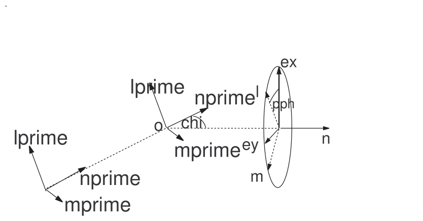
Figure 1: The incident photon direction ${\bf n}^{\prime}$, and scattered photon direction, ${\bf n},$ define athe scattering plane. ${\bf l}^{\prime}$ is taken to be the normal to the scattering plane, and ${\bf m}^{\prime}$ completes the right hand frame $\{{\bf l}^{\prime},{\bf m}^{\prime},{\bf n}^{\prime}\}$ for the incident photon. The scattered photon frame is defined by the right hand frame $\{{\bf l},{\bf m},{\bf n}\},$ where ${\bf l}$ is taken to be equal to ${\bf l}^{\prime}.$

We denote by ${\bf I}^{\prime}$ the Stokes parameters for incoming photons measured in the frame $\{{\bf l}^{\prime},{\bf m}^{\prime},{\bf n}^{\prime}\}$ . Incoming photons in solid angle $d\Omega_{{\bf n}^{\prime}}$ scattered into direction ${\bf n}$ give a contribution, $d{\bf I}({\bf r},{\bf n})$, per unit volume to the scattered intensities in frame $\{{\bf l},{\bf m},{\bf n}\}$ given by $d{\bf I}=\sigma n({\bf r})\SS({\bf n},{\bf n}^{\prime}){\bf I}^{\prime}({\bf r},{\bf n}^{\prime})d\Omega_{{\bf n}^{\prime}}.$ This defines the scattering phase function $\SS({\bf n},{\bf n}^{\prime})$. To integrate the different contributions to the scattered intensities from different incoming rays, we need to express all the scattered Stokes intensities in the same fixed reference frame. We take this fixed frame to be the observer’s frame $\{{\bf e}_{x},{\bf e}_{y},{\bf e}_{z}\}$, which is chosen such that ${\bf e}_{z}$ is the direction from the galaxy to the observer, ${\bf e}_{x}$ lies in the plane of the axis of symmetry of the galaxy and the line of sight, and ${\bf e}_{y}$ completes the right hand basis. Since in this context we are only interested in photons scattered towards the observer, we may without loss of generality put ${\bf n}={\bf e}_{z}$. Thus in order to sum the contributions from different beams we need to rotate from basis $\{{\bf l},{\bf m},{\bf n}\}$ to $\{{\bf e}_{x},{\bf e}_{y},{\bf e}_{z}\}$, that is through and angle $\tilde{\phi}$ given by $\cos\tilde{\phi}={\bf e}_{y}\cdot\ {\bf m}.$ Under such rotations the Stokes parameters transform as

$$\tilde{{\bf I}}={\bf R}(\tilde{\phi}){\bf I}$$ (10)

where

$${\bf R}=\begin{pmatrix}1&0&0&0\\ 0&\cos 2\tilde{\phi}&-\sin 2\tilde{\phi}&0\\ 0&\sin 2\tilde{\phi}&\cos 2\tilde{\phi}&0\\ 0&0&0&1\end{pmatrix}.$$ (11)

Thus equation(8) becomes

$$\begin{split}{\bf I}({\bf r},{\bf n})={\bf I}_{0}({\bf r},{\bf n})+\sigma\int_{-\infty}^{s}ds^{\prime}n({\bf r}^{\prime})\int_{4\pi}{\bf R}(\tilde{\phi})\SS({\bf n},{\bf n}^{\prime}){\bf I}({\bf r}^{\prime},{\bf n}^{\prime})d\Omega_{{\bf n}^{\prime}}\\ -\int_{0}^{s}n({\bf r}^{\prime})\sigma{\bf I}({\bf r}^{\prime},{\bf n})ds^{\prime},\end{split}$$ (12)

where ${\bf I}_{0}({\bf r},{\bf n})=\int^{s}_{-\infty}{\bf C}_{\rm stars}({\bf r}^{\prime},{\bf n})ds^{\prime}$ is the intensity at ${\bf r}$ in the direction ${\bf n}$ (i.e.when no scattering or absorption is present). (Any cylindrical distribution, $\rho(R,z)$, of stars, which we assume also radiate unpolarized radiation, must necessarily give rise to a source field, ${\bf I}_{0}({\bf r},{\bf n})$, that is cylindrically symmetric and unpolarized.) We may easily express the source intensities in terms of $\rho(R,z)$. Indeed, from figure 2 it can be seen that

$${\bf I}_{0}({\bf r},{\bf n})=\frac{L}{4\pi}(\int_{0}^{\infty}\rho({\bf r}-s{\bf n})ds,0,0,0).$$ (13)

It is convenient to introduce the normalised stellar density,

$$\tilde{\rho}=\frac{\rho}{\int\rho d^{3}{\bf r}}.$$ (14)

Equation 13 can then be written

$${\bf I}_{0}({\bf r},{\bf n})=\frac{L_{G}}{4\pi}(\int_{0}^{\infty}\tilde{\rho}({\bf r}-s{\bf n})ds,0,0,0),$$ (15)

where $L_{G}$ is the galaxy’s luminosity. Let us define the normalised source intensity

$$\Sigma({\bf r},{\bf n})=\frac{4\pi}{L_{G}}{\bf I}_{0}({\bf r},{\bf n}).$$ (16)

$\Sigma({\bf r},{\bf n})$ is essentially a stellar surface density.

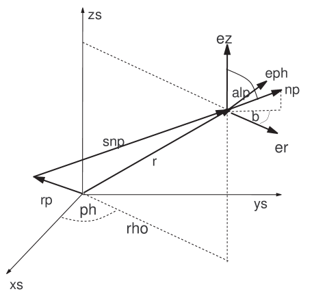
Figure 2: The intensity in direction ${\bf n}^{\prime}$ at $rr$ due to stellar distribution is obtained by integrating the stellar density along the line in the direction of ${\bf n}^{\prime}.$ The axis of symmetry is $Z.$ The polar and azimuthal angles of ${\bf n}^{\prime}$ in the the cylindrical frame are given by $\alpha$ and $\beta$ respectively.

We shall consider several scattering mechanisms. For Thomson scattering by electrons the scattering phase function $\SS$ takes the form

$$\SS=\frac{3}{16\pi}\begin{pmatrix}1+\cos^{2}\chi&\sin^{2}\chi&0&0\\ \sin^{2}\chi&1+\cos^{2}\chi&0&0\\ 0&0&2\cos\chi&0\\ 0&0&0&2\cos\chi\end{pmatrix}$$ (17)

In the case of Rayleigh scattering (molecules and small dust particles) the form of the scattering phase function is the same. However the total scattering cross section behaves as $\sigma\propto\lambda^{-4}$.

In many numerical simulations the Henyey–Greenstein form for scattering is used as an approximation to a typical mix of galactic dust particles.

In this case the scattering matrix takes the form

$${\bf S}_{hg}=\frac{1}{4\pi}\begin{pmatrix}P_{1}&P_{2}&0&0\\ P_{2}&P_{1}&0&0\\ 0&0&P_{3}&-P_{4}\\ 0&0&P_{4}&P_{3}\end{pmatrix}.$$ (18)

where

$$P_{1}=\frac{1-g^{2}}{(1+g^{2}-2\,g\,c_{\chi})^{3/2}}$$

and $P_{2}$ is given by

$$\frac{P_{2}}{P_{1}}=-p_{max}\frac{1-c_{\chi}^{2}}{1+c_{\chi}^{2}}$$

$P_{3}$ and $P_{4}$ are irrelevant for our study, since we are only concerned with unpolarized incident light. The single parameter $g$, which represents the mean value of the cosine of the scattering angle, determines how peaked in the forward direction the scattering is. $p_{max}$ is the peak polarization (i.e. the polarization at $90^{o}$). For the scattering of optical light on dust, $g$ and $p_{max}$ are both of the order of $0.5$ [White 1979]. We use these values in all our numerical calculations. Throughout, we have assumed that there is no absorption and that attenuation is purely due to scattering, corresponding to the case of albedo 1.

4 The optically thin approximation

If the galaxy is optically thin, in the sense that $\int n\sigma dl$ through the galaxy is less than one in all directions, then the first term on the right hand side of equation (12) will dominate. The optically thin approximation is obtained from first order iteration, in which ${\bf I}({\bf r},{\bf n}^{\prime})$ in the integral over solid angles in the second term, and ${\bf I}_{0}({\bf r},{\bf n}^{\prime})$ in the third term are replaced by and ${\bf I}_{0}({\bf r},{\bf n}^{\prime})$ and ${\bf I}_{0}({\bf r},{\bf n})$ respectively. Let us introduce the notation $d\tau_{z}=\sigma n({\bf r})dz.$ Thus in the optically thin approximation the asymptotic Stokes intensities in the direction of the observer, ${\bf I}(x,y,\infty,{\bf e}_{z})$, are given by

$$\begin{split}{\bf I}(x,y,\infty,{\bf e}_{z})={\bf I}_{0}{(x,y,\infty,{\bf e}_{z})}+\int_{0}^{\tau(x,y)}d\tau_{z}\int_{4\pi}{\bf R}(\tilde{\phi})\SS({\bf e}_{z},{\bf n}^{\prime}){\bf I}_{0}{({\bf r},{\bf n}^{\prime})}d\Omega_{{\bf n}^{\prime}}\\ -\int_{0}^{\tau(x,y)}{\bf I}_{0}({\bf r},{\bf e}_{z})\,d\tau_{z}.\end{split}$$ (19)

where $\tau(x,y)$ is the optical depth through the galaxy at the field point $(x,y).$

Writing equation (4) in component form, and introducing the elements $s_{ij}$ of the scattering phase function, $\SS$, we obtain

$$\begin{split}I(x,y,\infty,{\bf e}_{z})=I_{0}(x,y,\infty)+\int_{0}^{\tau(x,y)}d\tau_{z}\int_{4\pi}s_{11}({\bf n},{\bf n}^{\prime})I_{0}({\bf r},{\bf n}^{\prime})d\Omega_{{\bf n}^{\prime}}\\ -\int_{0}^{\tau(x,y)}I_{0}({\bf r},{\bf e}_{z})d\tau_{z}\end{split}$$ (20)

$$Q(x,y,\infty,{\bf e}_{z})=\int d\tau_{z}\int_{4\pi}d\Omega_{{\bf n}^{\prime}}I_{0}({\bf r},{\bf n}^{\prime})(s_{21}({\bf n},{\bf n}^{\prime})\cos 2\tilde{\phi}-s_{31}({\bf n},{\bf n}^{\prime})\sin 2\tilde{\phi})$$ (21)

$$U(x,y,\infty,{\bf e}_{z})=\int d\tau_{z}\int_{4\pi}d\Omega_{{\bf n}^{\prime}}I_{0}({\bf r},{\bf n}^{\prime})(s_{21}({\bf n},{\bf n}^{\prime})\sin 2\tilde{\phi}+s_{31}({\bf n},{\bf n}^{\prime})\cos 2\tilde{\phi})$$ (22)

and

$$V(x,y,\infty,{\bf e}_{z})=\int d\tau_{z}\int_{4\pi}d\Omega_{{\bf n}^{\prime}}I_{0}({\bf r},{\bf n}^{\prime})s_{41}({\bf n},{\bf n}^{\prime})$$ (23)

where $I_{0}$ is given in terms of the stellar number density by equation (13). Introducing the notation

$$W=Q+iU$$ (24)

we obtain

$$W(x,y,\infty,{\bf e}_{z})=\int d\tau_{z}\int_{4\pi}d\Omega_{{\bf n}^{\prime}}I_{0}({\bf r},{\bf n}^{\prime})\exp{i2\tilde{\phi}}((s_{21}({\bf n},{\bf n}^{\prime})+is_{31}({\bf n},{\bf n}^{\prime})).$$ (25)

In the case of spherical scattering, where the angular dependence of $s_{ij}$ is only in the scattering angle, $\theta$, one can expand $s_{11}$ ($s_{41}=0$ in this case) in terms of Legendre polynomials $P_{l}$, and $s_{21}$ and $s_{31}$ in terms of associated Legendre polynomials, $P_{lm}$ with $m=2$. This leads to simple expressions for the asymptotic Stokes intensities in terms of the line integrals of the multipole moments of the ${\bf I}_{0}({\bf r},{\bf n})$, with $m=0$ for the $I$ and $V$ and $m=2$ for $Z$. This is similar to the results obtained by [Simmons1982] and [Simmons1983] for the point source case. For Thomson and Rayleigh scattering further simplification results from the fact that only terms with $l=0,2$ occur in the expansion of the phase functions $s_{ij}$. This has a crucial importance when we come to calculate the flux. We shall not pursue this line of reasoning here, but rather adopt the simpler approach adapted to the case of Thomson and Rayleigh scattering. However, we outline the method using spherical harmonics section 4.3.

4.1 Polarization map

Using equations 20–23, it is possible to compute polarization maps of the galaxy. To carry out this we have divided the galaxy field into $100\times 100$ pixels, and for each each pixel we have integrated along the line of sight. The results our shown in figure (3), and can be seen to be comparable with those obtained by Wood [Wood 1997], who used Monte Carlo techniques. Of course the integration is in our case extremely quick. The degree of polarization is much higher for a galaxy viewed edge on than for the same galaxy viewed face on, and this is essentially due to the respective optical depths. One should note that for Henyey–Greenstein scattering the upper and lower half of the galaxy polarization is no longer symmetric. This is due to the functional form of the scattering, which is now peaked in the forward direction.

One can obtain the polarized flux from the polarization intensity maps by integrating the contributions to the polarization over the field of view. However, as we show in the sections 4.2 and 4.3, analytic expressions for the polarized flux in the case of Thomson and Rayleigh scattering can be found, and approximate expressions for general spherical scattering mechanisms.

Figure 3: Polarisation maps for Thomson scattering (bottom plots) and Henyey–Greenstein scattering (top plots). The inclinations of the galaxy are $87^{o}$, $60^{o}$ and $18^{o}$ for the left, central and right plots respectively. The degree of polarization is proportional to the length of the lines, the maximum polarization being 0.8% , 0.5% and 0.2% for the top row and 1.8%, 1.1% and 0.4% for the bottom row. The axis a labelled in $kpc$.

Figure 4: Polarization profile along the major axis of a galaxy for Thomson scattering for an inclination $87^{o}$. For Henyey–Greenstein the profile is very similar but the overall degree of polarization lower. The cut-off at $\pm 20kpc$ corresponds to the cut-off we have applied in the disc distribution, but the intensity at this distance from the galactic centre is already extremely low

4.2 Polarized flux for Thomson and Rayleigh scattering

The flux at the earth is obtained by integrating the asymptotic intensities, i.e. ${\bf I}(x,y,\infty,{\bf e}_{z})$, for large $s$ over all solid angles as seen by the observer. Noting that this solid angle is just given by $dxdy/R_{E}^{2}$ it is clear that integration of equation (12) over solid angles gives an expression for the flux in terms of volume integrals and the direct flux, ${\bf F}_{0}(\infty)$.

$$\begin{split}{\bf F}=\frac{1}{R_{E}^{2}}\int{\bf I}(x,y,\infty,{\bf e}_{z})dxdy={\bf F}_{0}+\int dV\sigma n({\bf r})\int{\bf R}(\tilde{\phi})\SS({\bf e}_{z},{\bf n}^{\prime}){\bf I}_{0}({\bf r},{\bf n}^{\prime})d\Omega_{{\bf n}^{\prime}}\\ -\int\sigma n({\bf r}){\bf I}_{0}({\bf r},{\bf e}_{z})dV.\\ \end{split}$$ (26)

From equation (15) it follows that

$${\bf F}_{0}(\infty)=\frac{L_{G}}{4\pi R_{E}^{2}}(1,0,0,0)$$ (27)

When calculating the degree of polarization to first order in optical depth, we need only normalize $F_{U}$ and $F_{Q}$ by the direct unpolarized flux, ignoring the contribution to the unpolarized flux from scattering.

Let us now assume that the galaxy has axial symmetry. Thus the distribution of stars and the density distribution of scatterers are taken to be cylindrically symmetric about this axis. The axis of symmetry is inclined at an angle of $i$ to the line of sight. It is useful to introduce cylindrical coordinates with origin at the centre of the galaxy, $\{R,\Phi,Z\}$ , with the $Z$ direction oriented along the axis of symmetry of the galaxy. (See figure 5 .)

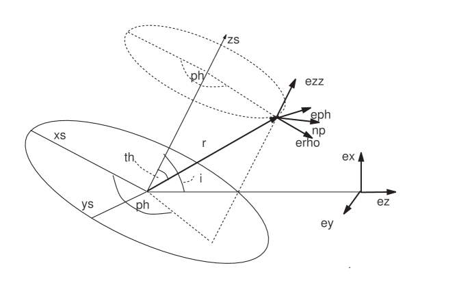
Figure 5: The axis of symmetry, given by $Z$, is inclined at angle $i$ to the line of sight. The observer’s frame is $\{{\bf e}_{x},{\bf e}_{y},{\bf e}_{z}\}$. $OX$, $OZ$ and ${\bf e}_{x}$ are taken to lie in the same plane.

It is also convenient to write $n=n_{0}\;\tilde{n},$ where $n_{0}$ is the central density of scatterers, and $\tilde{n}$ thus a dimensionless density. We introduce further a length scale $Z_{g}$ and the dimensionless variable $Z^{\prime}=Z/Z_{g}$, which will enable us to express the Stokes fluxes in terms of the optical depth, $\tau_{0}=n_{0}\sigma Z_{g}$. This is indeed the vertical optical depth for the models of section 2. We shall also work with the normalised intensity, $\Sigma({\bf r},{\bf n}),$ given by equation 16.

Because of the symmetry, the density of scatterers, $\tilde{n}$, is only be a function of $R$ and $Z$. Indeed this is the form assumed in the models of section 2. Similarly the unpolarized source Stokes intensity, $\Sigma({\bf r},{\bf n}),$ is a function of $R$ and $Z$, and the direction cosines, $\alpha,\beta$ of ${\bf n}^{\prime}$, expressed in terms of the associated coordinated basis vectors $\{{\bf e}_{R},{\bf e}_{\Phi},{\bf e}_{Z}\}$.

We shall now prove that under these assumptions, and with the additional assumption that the dust is optically thin, $F_{Q}$ depends only on $\sin^{2}i$, and $F_{U}=0$, generalizing the result obtained [Brown et al. 1977] for point sources. The behaviour of the degree of polarization will differ slightly from this, since the normalization factor, $F_{I}$, also depends weakly on the inclination. However, to first order in the optical depth the result will still hold. We also obtain an explicit form for the polarized flux in terms of density moments. Equation (26) written in component form now becomes

$$\begin{split}F_{I}=F_{0}(\infty)+\frac{L_{G}}{4\pi}\frac{3\tau_{0}}{16\pi R_{E}^{2}}\int\tilde{n}(R,Z)RdRdZ^{\prime}d\phi\int(1+\cos^{2}\chi)\ \Sigma(R,z,\alpha,\beta)\ \sin\alpha\,d\alpha\,d\beta\\ -\int n(R,Z)\sigma I_{0}(R,Z,\alpha,\beta)dV\\ \end{split}$$ (28)

$$\begin{split}F_{Q}=\frac{L_{G}}{4\pi}\frac{3\tau_{0}}{16\pi R_{E}^{2}}\int\tilde{n}(R,Z)RdRdZ^{\prime}d\phi\int\sin^{2}\chi\;\Sigma(R,Z,\alpha,\beta)\cos 2\tilde{\phi}\ \sin\alpha\,d\alpha\,d\beta\\ \end{split}$$ (29)

and

$$\begin{split}F_{U}=\frac{L_{G}}{4\pi}\frac{3\tau_{0}}{16\pi R_{E}^{2}}\int\tilde{n}(R,Z)RdRdZ^{\prime}\ d\phi\int\sin^{2}\chi\;I_{0}(R,Z,\alpha,\beta)\sin 2\tilde{\phi}\ \sin\alpha\,d\alpha\,d\beta.\end{split}$$ (30)

To evaluate $F_{I},F_{Q}$ and $F_{U}$ we shall need to work out the scattering angle $\chi$ (between ${\bf n}={\bf e}_{z}$ and ${\bf n}^{\prime}$) and the rotation angle $\tilde{\phi}$ between the scattering plane and the observer’s $y$ axis in terms of $\Phi,\alpha,\beta$. (As we shall see, although we do not require an explicit expression for the scattering angle in terms of $\Phi,\alpha,\beta$ for the calculation of $F_{Q}$ and $F_{U}$, for the evaluation of $F_{I}$ we shall require it.)

In order to do this we need to express the basis $\{{\bf e}_{R},{\bf e}_{\Phi},{\bf e}_{Z}\}$ in terms of $\{{\bf e}_{x},{\bf e}_{y},{\bf e}_{z}\}$. Let us introduce the convenient shorthand notation for cosine, $\cos A=c_{A}$, and sine, $\sin A=s_{A}$.

$$\begin{pmatrix}{\bf e}_{R}\\ {\bf e}_{\Phi}\\ {\bf e}_{Z}\\ \end{pmatrix}=\begin{pmatrix}c_{\Phi}&s_{\Phi}&0\\ -s_{\Phi}&c_{\Phi}&0\\ 0&0&1\\ \end{pmatrix}\begin{pmatrix}c_{i}&0&s_{i}\\ 0&1&0\\ -s_{i}&0&c_{i}\\ \end{pmatrix}\begin{pmatrix}{\bf e}_{x}\\ {\bf e}_{y}\\ {\bf e}_{z}\\ \end{pmatrix}.$$ (31)

The first matrix on the right hand side represents a transformation from $\{{\bf e}_{R},{\bf e}_{\Phi},{\bf e}_{Z}\}$ to $\{{\bf e}_{X},{\bf e}_{Y},{\bf e}_{Z}\}$, and the second from $\{{\bf e}_{X},{\bf e}_{Y},{\bf e}_{Z}\}$ to $\{{\bf e}_{x},{\bf e}_{y},{\bf e}_{z}\}$.

Equation (31) simplifies to

$$\begin{pmatrix}{\bf e}_{R}\\ {\bf e}_{\Phi}\\ {\bf e}_{Z}\\ \end{pmatrix}=\begin{pmatrix}c_{\Phi}c_{i}&s_{\Phi}&-c_{\Phi}s_{i}\\ -s_{\Phi}c_{i}&c_{\Phi}&s_{\Phi}s_{i}\\ s_{i}&0&c_{i}\\ \end{pmatrix}\begin{pmatrix}{\bf e}_{x}\\ {\bf e}_{y}\\ {\bf e}_{z}\\ \end{pmatrix}.$$ (32)

Writing

$${\bf n}^{\prime}=\begin{pmatrix}s_{\alpha}c_{\beta}&s_{\alpha}s_{\beta}&c_{\alpha}\\ \end{pmatrix}\begin{pmatrix}{\bf e}_{R}\\ {\bf e}_{\Phi}\\ {\bf e}_{Z}\\ \end{pmatrix},$$ (33)

and using equation (32) we obtain

$$\begin{split}{\bf n}^{\prime}=(s_{\alpha}c_{\beta}c_{\Phi}c_{i}-s_{\alpha}s_{\beta}s_{\Phi}c_{i}+c_{\alpha}s_{i}){\bf e}_{x}\\ +(s_{\alpha}c_{\beta}s_{\Phi}+s_{\alpha}s_{\beta}c_{\Phi}){\bf e}_{y}\\ +(s_{\alpha}c_{\beta}c_{\Phi}s_{i}+s_{\alpha}s_{\beta}s_{\Phi}s_{i}+c_{\alpha}c_{i}){\bf e}_{z}\\ \end{split}$$ (34)

Noting that $\cos\tilde{\phi}=({\bf n}^{\prime}\times{\bf e}_{z})\cdot{\bf e}_{y}/|{\bf n}^{\prime}\times{\bf e}_{z}|$ and $\sin\tilde{\phi}=({\bf n}^{\prime}\times{\bf e}_{z})\cdot{\bf e}_{x}/|{\bf n}^{\prime}\times{\bf e}_{z}|$ we immediately obtain from equation (34)

$$\cos\tilde{\phi}=-\frac{c_{\alpha}s_{i}+s_{\alpha}c_{\beta}c_{\Phi}c_{i}-s_{\Phi}c_{i}s_{\alpha}s_{\beta}}{s_{\chi}}$$ (35)

and

$$\sin\tilde{\phi}=\frac{s_{\alpha}c_{\beta}s_{\Phi}+s_{\alpha}s_{\beta}c_{\Phi}}{s_{\chi}}.$$ (36)

The scattering angle, $\chi$, is given by $\cos\chi=({\bf n}^{\prime}\cdot{\bf e}_{z})$, and again from equation (34) we obtain

$$c_{\chi}=c_{\alpha}c_{i}-s_{\alpha}c_{\beta}c_{\Phi}s_{i}+s_{\alpha}s_{\Phi}s_{\beta}s_{i}.$$ (37)

Noting that $\cos 2\tilde{\phi}=\cos^{2}\tilde{\phi}-\sin^{2}\tilde{\phi}$, and $\sin 2\tilde{\phi}=2\cos\tilde{\phi}\sin\tilde{\phi}$ and using eqs. (35) and (36), we see that in the integrand of equations 29 and 30 the terms $\sin^{2}\chi\cos 2\tilde{\phi}$ and $\sin^{2}\chi\sin 2\tilde{\phi}$ simplify by virtue of the cancellation of the $\sin^{2}\chi$ terms, and yield respectively

$$\begin{split}s^{2}_{\chi}c_{2\tilde{\phi}}=(c_{\alpha}s_{i}+s_{\alpha}c_{\beta}c_{\Phi}c_{i}-s_{\Phi}c_{i}s_{\alpha}s_{\beta})^{2}-(s_{\alpha}c_{\beta}s_{\Phi}+s_{\alpha}s_{\beta}c_{\Phi})^{2},\end{split}$$ (38)

and

$$\begin{split}s^{2}_{\chi}s_{2\tilde{\phi}}=-2(c_{\alpha}s_{i}+s_{\alpha}c_{\beta}c_{\Phi}c_{i}-s_{\Phi}c_{i}s_{\alpha}s_{\beta})(s_{\alpha}c_{\beta}s_{\Phi}+s_{\alpha}s_{\beta}c_{\Phi}).\end{split}$$ (39)

Upon carrying out the integration over $\Phi$ all terms in $\sin\Phi$, $\cos\Phi$, and $\sin 2\Phi$ disappear, since both $n$ and $I$ are independent of $\Phi$. A calculation shows that only terms with the factor $\sin^{2}i$ remain in the final expression for $F_{Q}$, and $F_{U}=0$. The latter implies that the polarization is in the y direction or in the x direction, i.e. along or perpendicular to plane defined by the axis of symmetry and the line of sight. Explicitly we obtain

$$\begin{split}F_{Q}=\frac{L_{G}}{4\pi}\frac{\tau\sin^{2}i}{16R_{E}^{2}}&\int\tilde{n}(R,Z)RdRdZ^{\prime}\int I_{0}(R,Z,\alpha,\beta)(3c_{\alpha}^{2}-1)\ s_{\alpha}\,d\beta d\alpha.\end{split}$$ (40)

Equation (40) has a simple interpretation: the polarized flux is proportional to the dipole moment of the radiation field weighted over the density distribution of the scatterers.

A similar calculation can be carried out for the unpolarized flux. Substituting in equation (28) the expression for $\cos\chi$ given in equation (37), we obtain

$$\begin{split}F_{I}=F_{0}(\infty)+\frac{L_{G}}{4\pi}\frac{3\tau_{0}\sin^{2}i}{16R_{E}^{2}}\int\tilde{n}(R,Z)R\ dR\ dZ^{\prime}\int I_{0}(R,Z,\alpha,\beta)(2+2c_{\alpha}^{2}c_{i}^{2}-s_{\alpha}^{2}s_{i}^{2}c_{2\beta})\ s_{\alpha}d\beta d\alpha\\ -\int n(R,Z)\sigma I_{0}(R,Z,\alpha,\beta)\ dV.\end{split}$$ (41)

The degree of linear polarization, $p$, is given, to first order in the optical depth, as $F_{Q}/F_{0}(\infty)$. From equations (40)and (27) we obtain

$$p=\frac{3\pi\tau_{0}\sin^{2}i}{16}\int RdRdZ^{\prime}n(R,Z)\int\Sigma(R,Z,\alpha,\beta)(3c_{\alpha}^{2}-1)\ s_{\alpha}d\beta d\alpha$$ (42)

where $\Sigma(R,Z,\alpha,\beta)$ is given by equation 16.

4.3 Approximate expressions for polarized flux using spherical harmonics

For more general mechanisms than Thomson and Rayleigh scattering the analytic methods used in section 4.2 are not very helpful. The approach used there worked because of the cancellation of the factor $\sin^{2}\chi$ in the integrand of the polarized fluxes owing to the form of the scattering phase function. For most phase functions this will not be the case.

Spherical harmonics, $Y_{lm}(\theta,\phi)$, provide us with a very powerful method of dealing with the general case. On the one hand they provide a complete set of orthogonal functions on the sphere, and on the other for each value of $l$ the $2l+1$ function $Y_{lm}(\theta,\phi)$ provide an irreducible representation of the rotation group. We shall largely follow the notation of Messiah (1961), and take the spherical harmonics to be defined by

$$Y_{lm}(\theta,\phi)=c(l,m)\ P_{l}^{m}(\cos\theta)e^{im\phi}\ \ {\rm where}\ \ c(l,m)=[\frac{(2l+1)(l-m)!}{4\pi(l+m)!}]^{1/2}$$ (43)

and $P_{l}^{m}$ are the associated Legendre polynomials. $c(l,m)$ is a normalisation constant to ensure $Y_{lm}(\theta,\phi)$ are orthonormal.

Thus suppose that we have two coordinate bases, $\{{\bf e}_{x},{\bf e}_{y},{\bf e}_{z}\}$ and $\{{\bf e}_{x}^{\prime},{\bf e}_{y}^{\prime},{\bf e}_{z}^{\prime}\}$. Suppose further that the rotation taking $\{{\bf e}_{x},{\bf e}_{y},{\bf e}_{z}\}$ into $\{{\bf e}_{x}^{\prime},{\bf e}_{y}^{\prime},{\bf e}_{z}^{\prime}\}$ is described by the Euler angles $A,B,C$. We then have the relation

$$Y_{lm}(\theta^{\prime},\phi^{\prime})=\sum_{m^{\prime}=-l}^{m^{\prime}=l}Y_{lm^{\prime}}(\theta,\phi)R^{(l)}_{m^{\prime}m}(A,B,C).$$ (44)

The matrices ${\bf R}^{(l)}$ form an irreducible representation of the rotation group. The elements of ${\bf R}^{(l)}$ take the form

$$R^{(l)}_{mm^{\prime}}(A,B,C)=e^{-imA}r^{(l)}_{mm^{\prime}}(B)e^{-im^{\prime}C},$$ (45)

where $r^{(l)}_{m^{\prime}m}(B)$ can be calculated from the Wigner formula (see Messiah 1961),

$$r^{(l)}_{mm^{\prime}}=\sum_{t}(-1)^{t}\frac{\sqrt{(l+m)!(l-m)!(l+m^{\prime})!(l-m^{\prime})!}}{(l+m-t)!(l-m^{\prime}-t)!t!(t-m+m^{\prime})!}\xi^{2l+m-m^{\prime}-2t}\eta^{2t-m+m^{\prime}},$$ (46)

where $\xi=\cos B/2$ and $\eta=\sin B/2$.

It is convenient for our purposes to work entirely in the observer’s reference frame (see figure (5). Our two frames are thus $\{{\bf e}_{x},{\bf e}_{y},{\bf e}_{z}\}$, the observer’s frame, and $\{{\bf e}_{x}^{\prime},{\bf e}_{y}^{\prime},{\bf e}_{z}^{\prime}\}=\{{\bf e}_{R},{\bf e}_{\Phi},{\bf e}_{Z}\}$, the frame attached to the galaxy’s cylindrical coordinates. With this notation we replace $\theta^{\prime}$ by $\alpha$, and $\phi^{\prime}$ by $\beta.$ To rotate the coordinate basis $\{{\bf e}_{x},{\bf e}_{y},{\bf e}_{z}\}$ into $\{{\bf e}_{R},{\bf e}_{\Phi},{\bf e}_{Z}\}$ we have to

(i) rotate about $y$-axis though $i$ and then

(ii)rotate about $Z$-axis though $\Phi$. Thus $A=0$, $B=i$, and $C=\Phi.$

Let us assume that the source Stokes intensity has cylindrical symmetry, i.e. $I_{0}=I_{0}(R,Z,\alpha,\beta)$. Let us work in terms of the normalised surface density $\Sigma(R,Z,\alpha,\beta)={4\pi}I_{0}(R,Z,\alpha,\beta)/{L_{G}}$ as defined in equation 16. Expanding $\Sigma(R,Z,\alpha,\beta)$ in terms of spherical harmonics

$$\Sigma(R,Z,\alpha,\beta)=\sum_{l=0}^{l=\infty}\sum_{m=-l}^{m=l}a_{lm}(R,Z)Y_{lm}(\alpha,\beta)$$ (47)

where of course $a_{lm}$ do not depend on $\Phi$. Indeed because of the orthogonality of the spherical harmonics we may write

$$a_{lm}(R,Z)=\int_{4\pi}\Sigma(R,Z,\alpha,\beta)Y_{lm}^{*}(\alpha,\beta)d\Omega.$$ (48)

Now expressing $Y_{lm}(\alpha,\beta)$ in terms of $Y_{lm}(\theta,\phi)$ via equation 44, and substituting into equation 47, we obtain

$$\Sigma(R,Z,\alpha,\beta)=\sum_{l=0}^{l=\infty}\sum_{m=-l}^{m=l}\sum_{m^{\prime}=-l}^{m^{\prime}=l}a_{lm}(R,Z)Y_{lm^{\prime}}(\theta,\phi)R^{(l)}_{m^{\prime}m}(0,i,\Phi).$$ (49)

Now from equation representation, $R^{(l)}_{m^{\prime}m}(0,i,\Phi)=r^{(l)}_{m^{\prime}m}(i)\exp{-im\Phi}$.

The angle ( denoted by $\tilde{\phi}$ in figure 1) between the scattering plane of the incoming photon in direction ${\bf n}$, and the observer’s $x-z$ plane, is $\tilde{\phi}=\phi-\pi/2$, and the scattering angle, $\chi$ in the main text, is $\chi=\theta$.

The complex intensity, $W$, is given by equation 25 . Note that for spherical scattering mechanisms we need only consider $s_{21}$ and moreover $s_{21}=s_{21}(\theta)$. To obtain the polarized flux, expression (25) for the complex intensity, $W=Q+iU$, has to be integrated over all solid angles at the observer. As in section (4.2) we multiply by the element of solid angle, $dxdy/R_{E}^{2}$, thus transforming the expression (25) into a volume integral, where we have written $d\tau_{z}=\sigma n_{0}\tilde{n}dz$ .

As before, introducing the dimensionless variable $Z^{\prime}=Z/Z_{g}$, and the central optical depth, $d\tau_{0}$, we thus obtain the expression

$$F_{Q}+iF_{U}=-\frac{\tau_{0}L_{G}}{4\pi R_{E}^{2}}\int\tilde{n}(R,Z)RdRdZ^{\prime}d\Phi\int s_{21}(\theta)\Sigma(R,Z,\alpha,\beta)e^{i2\phi}\sin\theta d\theta d\phi.$$ (50)

Substituting equation (49) into equation (50) we obtain

$$\begin{split}F_{Q}+iF_{U}=-\frac{\tau_{0}L_{G}}{4\pi R_{E}^{2}}\int\tilde{n}(R,Z)RdR\ dZ^{\prime}d\Phi\int s_{21}(\theta)\sum_{l=0}^{l=\infty}\sum_{m=-l}^{m=l}\sum_{m^{\prime}=-l}^{m^{\prime}=l}\\ a_{lm}(R,Z)Y_{lm^{\prime}}(\theta,\phi)r^{(l)}_{m^{\prime}m}(i)e^{-im\Phi}e^{i2\phi}\sin\theta d\theta d\phi\end{split}$$ (51)

Integration over $\Phi$ eliminates all terms for which $m\neq 0$, and introduces a factor $2\pi$ for $m=0$. With the definition

$$A_{lm}=\int\tilde{n}(R,Z)\,a_{lm}(R,Z)\,R\,dR\,dZ^{\prime}$$ (52)

equation (51) reduces to

$$\begin{split}F_{Q}+iF_{U}=-\frac{L_{G}\tau_{0}}{2R_{E}^{2}}\sum_{l=0}^{l=\infty}A_{l0}\sum_{m^{\prime}=-l}^{m^{\prime}=l}\int s_{21}(\theta)Y_{lm^{\prime}}(\theta,\phi)r^{(l)}_{m^{\prime}0}(i)e^{i2\phi}\sin\theta d\theta d\phi.\end{split}$$ (53)

Clearly, only the term $m^{\prime}=-2$ can contribute, and integral (53) reduces to

$$F_{Q}+iF_{U}=-\frac{L_{G}\tau_{0}}{2R_{E}^{2}}\sum_{l=2}^{l=\infty}A_{l0}r^{(l)}_{-20}(i)S_{l2\ (21)}$$ (54)

where

$$S_{l2\ (21)}=2\pi\ c(l,-2)\int s_{21}(\theta)P_{l\,2}(\cos\theta)\sin\theta d\theta.$$ (55)

Since all the terms on the right hand side equation (54) are real, it follows that $F_{U}$ is zero, meaning that the polarization is either directed along the axis of symmetry, or perpendicular to it. For Thomson scattering the only non-zero term in the multipole expansion of the phase function is $S_{22\ (21)}$, and we obtain the result proved in 4.2, since $r^{(2)}_{-20}(i)$ is proportional to $\sin^{2}i$. On the other hand, if the scattering phase function has higher multipoles, then the dependence of the polarization on the inclination angle will have higher terms in $\sin i$ and $\cos i$.

To first order in optical depth, the degree of polarization is given by, $p=|F_{Q}|/F_{0}(\infty)$. Noting that $F_{0}(\infty)=L_{G}/4\pi R_{E}^{2}$ we obtain for the degree of polarization

$$p=2\pi\tau_{0}\sum_{l=2}^{l=\infty}A_{l0}\;r^{(l)}_{-20}(i)S_{l2}$$ (56)

A similar calculation can be carried out for $F_{I}$.

4.4 Dependence of polarized flux on inclination

From the polarization maps presented in section (4.1), it is possible to calculate the integrated degree of polarization over the entire galaxy. This must be a function of the inclination. The corresponding plots of polarization (calculated in this way) against inclination are given in figure (6). For Thomson scattering one obtains the $\sin^{2}i$ law, as expected from the analytic results of section 4.2. On the other hand, for Henyey–Greenstein scattering, there is a noticeable deviation from this law.

The dependence of the total polarization on inclination can also be calculated using the expansion in spherical harmonics outlined in the previous section. The degree of polarization is given by equation 56.

$A_{l0}$ is an integral over the distribution of stars, dust and gas, and does not depend on the scattering mechanisms or inclination. $r^{(l)}_{-20}$ is a function of inclination that is easy to calculate. $S_{l2\ (21)}$ is determined from the scattering function from the simple integral given by equation 55.Results for $l=2,3$ and $4$ are shown in the table 1. For Thomson scattering only $l=2$ is non-zero. For Henyey–Greenstein higher order multipoles are not zero, nevertheless, as is illustrated in figure (6), even with inclusion only of the $l=2$ term a very good fit is found. Including terms up to $l=4$, one obtains an excellent fit to the numerical results, with a disagreement of only a few percent.

Evidently this method can test an arbitrarily large number of different scattering mechanisms and geometries extremely quickly, since the total polarization is given by a simple sum of products of easily calculated terms. Thus to see the effect of changing the scattering mechanism, it is sufficient to simply recalculate the corresponding coefficients $S_{l2\ (21)}.$

	$r^{(l)}_{-20}$	$A^{\prime}_{l0}$	$S_{l2\ (21)}$ (thom.)	$S_{l2\ (21)}$ (HG)
l=2	$\frac{\sqrt{24}}{8}\sin^{2}(i)$	$2.21\;10^{-2}$	$\sqrt{3\pi/10}$	$0.373$
l=3	$\frac{\sqrt{30}}{4}\sin^{2}(i)\cos(i)$	$-4.16\;10^{-3}$	$0.$	$0.174$
l=4	$\frac{\sqrt{10}}{16}\sin^{2}(i)(5+7\cos(2i))$	$-1.72\;10^{-2}$	$0.$	$0.043$

Table 1:

Figure 6: Degree of polarization as a function of $i$. The empty squares show the numerical values for Thomson scattering and the full squares for Henyey–Greenstein scattering. The $sin^{2}$ law is, as was expected, recovered for the Thomson scattering (solid line) . For the Henyey–Greenstein scattering there is a noticeable deviation from this law. The short-dashed line corresponds to the l=2 approximation, and the long-dashed line to the l=4 approximation for Henyey-Greenstein scattering.

5 Discussion and conclusions

The assumption that the spiral galaxy is optical thin allows us to easily calculate numerically the spatially resolved degree of polarization and unpolarized intensity of starlight scattered by dust, electrons and gas. Our numerical results agree qualitatively with the observations for spiral galaxies, and for vertical optical depths of around $0.05$ give maximum polarization of around 1% depending on the dominant scattering mechanism and inclination of the galaxy. For the same optical depth, Thomson and Rayleigh scattering are more efficient in producing polarization than the Henyey/Greenstein phase function. The latter produces an asymmetry in the polarization about the semi-major axis of the elliptical image of the galaxy.

Although we should expect the optical thin assumption might break down for high inclination galaxies, which are indeed the ones discussed by [Draper et al.1995] and [Scarrott et al. 1996], and where the optical depth along the galactic plane is greater than $1$, our results appear to agree well with the Monte Carlo calculations of a number of authors. It would be interesting to make a detailed comparison of the two methods.

The advantages of the optical thin assumption is undoubtedly its efficiency: the computer time needed for calculation of maps considerably less than Monte Carlo treatment. Although we have dealt only with Thomson and Henyey–Greenstein type scattering functions, the inclusion of mixtures of scatterers etc. would be very straightforward, and involve only slightly more computer time. It would is a straightforward extension to treat a case where the galaxy is optically thick in absorption, but optically thin in scattering. However in this case we should not expect the same inclination law to hold for the polarization. We shall deal with this case in a future paper. There have been only few observational studies of the polarization of the integrated flux from spiral galaxies. We find that in the optically thin regime, for Thomson or Rayleigh scattering, the dependence of the degree of polarization on inclination of the galactic axis to the line of sight, $i$, has a simple $\sin^{2}i$ form if we assume axial symmetry in both the distribution of scatterers and stars. Again, for vertical optical depths of $\tau\approx 0.05$, the total integrated polarization reaches about $1$% for higher inclinations.

Thus the suggestion that optical polarization could be used in the study of weak lensing [Audit & Simmons1999] is further supported by this study. Although the observation of such levels of polarization would be difficult in such high redshift galaxies, the more important determination of the direction of polarization might be feasible.

Such a technique, in determining the orientation of the source galaxy, would provide considerably more precision in determining the mass distribution in weak lensing studies.

For more complicated scattering mechanisms one can write down an expression for the total integrated polarization in terms of a spherical harmonic expansion expansion. For the class of galaxy models we have taken, it appears that the convergence of this expansion is very rapid, and that to a good approximation the polarization is given by the first term of the expansion, $l=2$. This indicates that the $\sin^{2}i$ law should be more generally applicable. Our formulation easily allows the inclusion of other mechanisms (absorption and dichroism etc.).

Although we have not investigated the the joint distribution of flux and polarized flux for a catalogue of spiral galaxies, it would be interesting to do so. In the optically thin regime we would expect a correlation between the two, whereas in the optically thick regime the flux should be independent of inclination. Thus this could provide a test for optical thickness for a class of spiral galaxies. The form of the joint distribution could also indicate whether scattering or other mechanisms just as alignment of grains by magnetic fields is responsible for polarization in a class of spiral galaxies.

Finally we would like to point out the possible use of polarization in a Faber-Jackson type distance estimators arising from the possible correlation between polarization and absolute magnitude of galaxies, which could be used to refine the distance scale for galaxies.

References

- [Audit & Simmons1999] Audit E. and Simmons J. F. L., 1999, MNRAS, 303, 87-95
- [Bianchi et al. 1996] Bianchi S., Ferra A. and Giovanardi C., 1996, ApJ, 465, 127-144
- [Bosma et al. 1992] Bosma A., Byun Y., Freeman K.C. and Athanassoula E., 1992, ApJ, 400, L21-L24
- [Brown et al. 1977] Brown J. C., McClean I. S. , 1977, A&A, 57 , 127-144
- [Byun et al.1994] Byun Y.I., Freeman K.C. and Kylafis N.D., ApJ 432, 116-127
- [Calzetti & Heckman1999] Calzetti D. and Heckman T. 1999, ApJ, 519, 27-47
- [Cassinelli et al. 1986] Cassinelli J., Brown J. C. and Carslaw V., 1986, ApJ, 465, 127-144
- [Draper et al.1995] Draper P.W., Done C., Scarrott S. M. and Stockdale D.P., 1995, MNRAS, 277, 1430–1434
- [Jaffe 1983] Jaffe W., 1983, MNRAS, 202, 995
- [Scarrott et al. 1996] Scarrott S. M., Foley N. B. and Gledhill T. M. and Wolstencroft R. D., 1996, MNRAS, 282, 252–262
- [Simmons1982] Simmons J. F. L., 1982, MNRAS, 200, 91-113
- [Simmons1983] Simmons J. F. L., 1983, MNRAS, 205, 153-170
- [White 1979] White R. L. , 1979, ApJ, 229, 954-961
- [Wood 1997] Wood K., 1997, Apj, 477, L25-L28
- [Wood & Jones 1997] Wood K. and Jones T. J., 1997, AJ, 114(4), 1405
- [Xilouris et al.1999] Xilouris E. M., Byun Y.I., Kylafis N.D., Paleologou E.V. and Papamastorakis J., 1999, A& A, 344, 868-878