How accurately can we measure weak gravitational shear?

Abstract

With the recent detection of cosmic shear, the most challenging effect of weak gravitational lensing has been observed. The main difficulties for this detection were the need for a large amount of high quality data and the control of systematics during the gravitational shear measurement process, in particular those coming from the Point Spread Function anisotropy.

In this paper we perform detailed simulations with the state-of-the-art algorithm developed by Kaiser, Squires and Broadhurst (KSB) to measure gravitational shear. We show that for realistic PSF profiles the KSB algorithm can recover any shear amplitude in the range $0.012<|{\mbox{\boldmath$\gamma$}}|<0.32$ with a relative, systematic error of $10-15\%$. We give quantitative limits on the PSF correction method as a function of shear strength, object size, signal-to-noise and PSF anisotropy amplitude, and we provide an automatic procedure to get a reliable object catalog for shear measurements out of the raw images.

Key words: Cosmology: theory, gravitational lenses

1 Introduction

Weak gravitational lensing has become one of the most important cosmological tools in the last decade. The mass distribution in the universe can in principle be mapped from the measurement of the coherent distortion caused by inhomogeneously distributed foreground mass on the orientation of the faint background galaxies. Lensing by clusters of galaxies, strong enough to be routinely detected now, already provides important constraints on the nature of our universe [e.g. it probed massive high-redshift clusters (Luppino & Kaiser 1997; LK97 henceforth; Clowe et al. 1998) and revealed the possible existence of dark clumps (Erben et al. 2000, Umetsu et al. 2000)]. Since the first publications of “cluster lensing” (see e.g., Tyson, Valdes & Wenk 1990 and Kaiser & Squires 1993) much theoretical and observational progress on weak lensing has been made, and interest progressively turned to very weak shear measurements. Galaxy-galaxy lensing is an example of such a study which provides constraints on average dark matter halo properties of galaxies, and cosmic shear is, ultimately, the direct measurement of statistical properties of the large-scale matter distribution in our universe (see, e.g., Schneider & Rix 1997, Schneider et al. 1998b). First galaxy-galaxy lensing experiments investigating dark halos of field and cluster galaxies have been successfully made (Brainerd, Blandford & Smail 1995, Fischer et al. 1999, Natarayan et al. 1998). Very recently, the cosmic shear was also detected (Schneider et al. 1998a, van Waerbeke et al. 2000, Bacon et al. 2000a, Wittmann et al. 2000, Kaiser et al. 2000). Because of the small amplitude of the lens effect, a quantitative analysis of the signal requires high-quality data and very precise data analysis for the detection of the signal. With the advent of new high-quality wide field CCD cameras substantial amounts of useable data for these studies will soon become available [e.g., the Descart project (http://terapix.iap.fr/Descart/Descart_english.html)].

On the analysis side, the key issue is the determination of the gravitational shear $\gamma$ measured from galaxy shapes. Using real data, we have to deal with observational and data reduction defects. On CCD images, the information from very faint and small objects whose shape we want to measure is often contained in only a few image pixels and a clear relation of pixels to individual objects is hard to achieve. Moreover, the measurements are rendered more difficult by pixel noise and PSF effects that can mimic a possible shear signal. Kaiser, Squires & Broadhurst (1995, KSB henceforth) have proposed a method for shear determination which is optimised for the analysis of faint and small objects by utilising weighted brightness moments of the light distribution. Their formalism (the so-called IMCAT) is to date one of the few taking into account smearing and anisotropy effects from an atmospheric PSF. Their formulae were derived for the weak-shear limit and assuming that PSFs can be written as an isotropic PSF convolved with a compact, anisotropic kernel. In this paper we investigate the accuracy and limitations of this method with simulations. We address the following questions: (1) It was shown in earlier publications that PSF profiles, for which the KSB breaks down, can be constructed very easily (Kuijken 1999). So, is the proposed PSF correction procedure valid for PSF profiles that we observe in ground-based observations? (2) What influence does pixel noise have on the shear estimation? (3) The KSB formulae are valid to first order in the shear ($\kappa\ll 1,\;|{\mbox{\boldmath$\gamma$}}|\ll 1$). Is this expansion valid for typical weak lensing applications with ground-based observations (from $|{\mbox{\boldmath$\gamma$}}|=0.01$ for cosmic shear up to $|{\mbox{\boldmath$\gamma$}}|=0.2$ for cluster mass reconstructions) or should we expand the formalism to higher order? (4) Can we set up a fully automatic procedure, from reduced images to an object catalog, for reliable shear measurements?

We generate a large number of simulated images and analyse them exactly in the same way as real data. We perform two kinds of simulations:

• Simulations where all objects involved (galaxies as well as stars) have Gaussian profiles.

• Simulations with the SkyMaker program (Bertin 2000, in preparation). This program generates galaxies modelled as exponential disks with a central de Vaucouleurs type bulge of varying ratio. The most important feature of SkyMaker is its ability to produce realistic ground-based PSFs and to allow for the inclusion of several telescope/detector defects (like astigmatism, coma, drift)

The outline of the paper is as follows: Sect. 2 summarises the KSB formalism and how we use it to estimate gravitational shear. Sect. 3 gives a short overview over the Stuff program which generates the input galaxy and star catalogs for the SkyMaker program. We describe our simulations with Gaussian profiles in Sect. 4, our object detection and selection procedure in Sect. 5. The SkyMaker simulations follow in Sect. 6 and we finish with our conclusions in Sect. 7. The generation of Point Spread Functions in the SkyMaker program is described in an Appendix.

2 Shear estimates

KSB estimates the shear by considering the first order effects of a gravitational shear and an instrumental Point Spread Function (PSF) on the (complex) ellipticity of the galaxies ${\mbox{\boldmath$\chi$}}=\chi_{1}+{\rm i}\chi_{2}$, which is defined as:

$$\chi_{1}=\frac{Q_{11}-Q_{22}}{Q_{11}+Q_{22}};\chi_{2}=\frac{2Q_{12}}{Q_{11}+Q_{22}},$$ (1)

where the $Q_{ij}$ are weighted second brightness moments of the light distribution $I$:

$$Q_{ij}=\int{\rm d}^{2}\theta\theta_{i}\theta_{j}I({\theta})W(|\theta|),$$ (2)

where the object centre is at the origin of the coordinate system, i.e.

$$\int{\rm d}^{2}\theta\theta I({\theta})W(|\theta|)=0.$$ (3)

The total response of the galaxy ellipticity $\hat{{\mbox{\boldmath$\chi$}}}^{0}$, that is the intrinsic ellipticity convolved with an isotropic function [see Bartelmann & Schneider (2000)], to a reduced gravitational shear ${\bf{g}}={\mbox{\boldmath$\gamma$}}/(1-\kappa)$ and the PSF is given by:

$${\mbox{\boldmath$\chi$}}-\hat{{\mbox{\boldmath$\chi$}}}^{0}=P^{\rm g}{\bf{g}}-P^{\rm sm}{\bf{q}}^{*};\;\;P^{\rm g}=P^{\rm sh}-P^{\rm sm}(P^{*\rm sm})^{-1}P^{*\rm sh},$$ (4)

where $\chi$ is the observed ellipticity and the tensors $P^{\rm sh}$ and $P^{\rm sm}$ can directly be calculated from the galaxy’s light profile and the weight function $W$. $P^{\rm sh}$ (Shear polarizability) would be the response of the weighted galaxy ellipticity to a gravitational shear in the absence of PSF effects. $P^{\rm g}$ modifies this tensor by a factor including the Smear polarizability tensor $P^{\rm sm}$ to calibrate the shear estimate for the circular smearing by the PSF. This calibration also depends on the corresponding tensors $P^{*\rm sh}$ and $P^{*\rm sm}$ from stellar objects containing the information of the PSF. The stellar anisotropy kernel ${\bf{q}}^{*}$, needed for the correction of the PSF anisotropy, can be estimated by noting that $\hat{{\mbox{\boldmath$\chi$}}^{0}}^{*}=0$, ${\bf{g}}^{*}=0$ for stars so that

$${\bf{q}}^{*}=(P^{*\rm sm})^{-1}{\mbox{\boldmath$\chi$}}^{*}.$$ (5)

A complete derivation of these formulae clarifying all the assumptions in the formalism is published in Bartelmann & Schneider (2000) but see also KSB, LK97 and Hoekstra et al. (1998). To estimate ${\bf{g}}$ we first correct objects for the PSF anisotropy:

$${\mbox{\boldmath$\chi$}}^{\rm aniso}={\mbox{\boldmath$\chi$}}+P^{\rm sm}{\bf{q}}^{*}$$ (6)

and then consider averages over galaxy images in areas where we assume constant reduced shear:

$$\langle{\mbox{\boldmath$\chi$}}^{\rm aniso}\rangle-\langle\hat{{\mbox{\boldmath$\chi$}}^{0}}\rangle=\langle P^{\rm g}{\bf{g}}\rangle=\langle P^{\rm g}\rangle\langle{\bf{g}}\rangle\rightarrow\langle{\bf{g}}\rangle={\langle P^{\rm g}\rangle^{-1}\langle{\mbox{\boldmath$\chi$}}^{\rm aniso}\rangle};\;\;$$ (7)

where we used $\langle\hat{{\mbox{\boldmath$\chi$}}^{0}}\rangle=0$. For simplicity eq. (4) is often used in the form:

$${\bf{g}}={(P^{\rm g})^{-1}}({{\mbox{\boldmath$\chi$}}^{\rm aniso}-\hat{{\mbox{\boldmath$\chi$}}^{0}}})\Rightarrow\langle{\bf{g}}\rangle=\left\langle{(P^{\rm g})^{-1}}{{\mbox{\boldmath$\chi$}}^{\rm aniso}}\right\rangle$$ (8)

where we have to assume $\langle{(P^{\rm g})^{-1}}{\hat{{\mbox{\boldmath$\chi$}}^{0}}}\rangle=0$. We checked that with our procedure described below this assumption holds and the estimators from eq. (7) and eq. (8) are in very good agreement, although in practice the latter is easier to handle.

2.1 Practical application of the KSB formulae

Although the general KSB procedure seems uniquely determined, there are several possibilities for its practical implementation. This has been the subject of discussions in recent works (Hoekstra et al. 1998, Kuijken 1999, Kaiser 1999) on how the KSB formulae should be applied optimally. One issue is the window function $W(|\theta|)$ with which galaxies are weighted. KSB have chosen a Gaussian with a scale $\sigma$ proportional to the size of the object under consideration. Hoekstra et al. (1998) noted first that quantities from stellar objects should be calculated with the same scale as the object to be corrected (this is the most natural choice although according to the derivation of the KSB formulation the result should not depend on it). Another difficulty arises as the quantities ${\bf{q}}^{*}$ and $(P^{*\rm sm})^{-1}P^{*\rm sh}$ have to be known at the positions of the galaxies to be corrected. Since these quantities are known only at star locations, we need to estimate what the PSF would be on the position of each detected galaxy. On top of all, all measured quantities are affected by noise in an unknown way. Two techniques have been proposed to suppress this noise in the shear estimate. First, the noise in the scaling factor $P^{\rm g}$ can be minimised by a fit or by calculating means or medians in bins in the parameter space $\pi_{P^{\rm g}}$=(object size, magnitude) which has often been used in the literature. Second, we can easily introduce a weighting scheme in the estimators (7) and (8).

Our procedure, which we found to be optimal in terms of shear recovery accuracy, can be summarised as follows: To apply (4), for every galaxy the quantities ${\bf{q}}^{*}$ and $(P^{*\rm sm})^{-1}P^{*\rm sh}$ have to be known everywhere on the image. Usually the PSF anisotropy varies smoothly over the field so that the $q^{*}_{i}$ can be well represented by a low-order polynomial fit from the light profiles of bright, unsaturated foreground stars. A second-order polynomial is enough, and higher order polynomials do not improve the PSF correction. We select these stars in a $r_{\rm h}$ vs. m diagram (see Fig. 1),

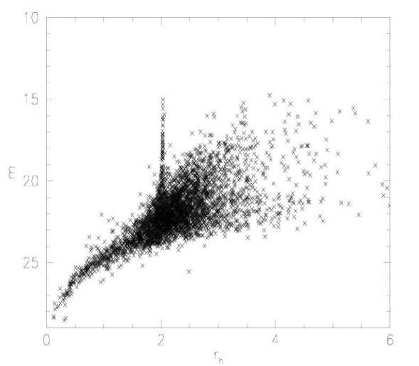
Fig. 1.: Plotted is the half light radius vs. the magnitude (in arbitrary units) from all the detections in one of our SkyMaker simulations in Sect. 6. Bright, unsaturated stars are clearly localised in a small region around $r_{h}\approx 2$ and in $15<{\rm m}<20$. Larger objects are considered as galaxies, while the smaller, very faint objects are probably noise detections. For objects around the stellar locus with faint magnitudes, a clear classification between stars and galaxies cannot be done and we typically exclude this region from our analysis.

and then measure ${\bf{q}}^{*}$ with a filter of the size of the stars, but $(P^{*\rm sm})^{-1}P^{*\rm sh}$ in a range of filter scales spanning the sizes of our galaxies. We then perform the anisotropy correction (6) for each individual galaxy. For $P^{\rm g}$ we finally use the raw, unsmoothed values as our analysis shows that fitting this quantity does not improve the final results (see Sect. 4).

Corrected galaxy ellipticities are subject to high noise, which can eventually produce unphysical ellipticities much larger than unity. It is therefore necessary to weight each galaxy according to the accuracy of its ellipticity measurement/correction. For our weighting scheme we assume the ellipticity distribution of the lensed galaxies is to first order equivalent to the intrinsic ellipticity distribution everywhere on our data field. We also assume that the intrinsic ellipticity distribution does not vary over the field. So, high ellipticities are assumed to originate from noise and these galaxies should be assigned a low weight. These assumptions are valid for studies of empty fields but not when investigating cluster lenses where high ellipticities are lensing features and not necessarily caused by noise. In this case a weighting scheme calculating weights out of the pixel noise properties may be adopted. See the Appendix of Hoekstra et al. (1999) for an example.

We introduce a simple $U=1/\sigma_{\rm g}^{2}$ weighting, where $\sigma_{\rm g}^{2}$ is the variance of the shear estimators from individual objects. These weights are estimated in a parameter space $\pi_{U}$ supposed to trace the noise properties of objects (like object size and S/N for example). Unfortunately our objects are typically very clustered in $\pi_{U}$ so that calculating averages in cells defined by a regular grid is not optimal and an adaptive grid should be more appropriate. Therefore for each galaxy we consider its $N$ nearest neighbours in our parameter space (typically $N\simeq 20$) and assign the inverse of $\sigma_{\rm g}^{2}=\frac{1}{N}\sum|{\bf{g}}|^{2}$ from these neighbours as weight to that galaxy. The distance $d$ from a galaxy $k$ to its neighbour $l$ in a parameter space $\pi$ consisting of $i=1..M$ elements is hereby defined by

$$d=\sqrt{\sum_{i=1}^{M}(\pi_{i}^{k}-\pi_{i}^{l})^{2}}.$$ (9)

Obviously, a galaxy does not have an unique set of closest neighbours in an arbitrary space. For instance, object sizes would simply scale by a factor of 2 if data are rebinned to half the original resolution while quantities like m stay unchanged. Possible consequences of this are not investigated here. Hereafter we denote averages $\langle x\rangle$ and uncertainties of means $\sigma_{\langle x\rangle}$ from a weighted quantity $x$ by:

$$\langle x\rangle = \frac{\sum_{k}x_{k}U_{k}}{\sum_{k}U_{k}};$$ (10)

$$\sigma_{\langle x\rangle}^{2} = \frac{1}{\sum_{k}U_{k}}.$$

As noted above, our weighting scheme is well justified only if the lensed ellipticity distribution is to first order equivalent to the unlensed one. We found in our simulations that we can also estimate shear that is not small with respect to the intrinsic ellipticity distribution with the above formulae but not the corresponding errors. The reason is that only relative weights enter the shear estimate while the errors $\sigma_{\langle x\rangle}^{2}$ are determined by the absolute values of the weights. In the strong shear case, that is, if the intrinsic ellipticity distribution is substantially changed by the input shear, the absolute values of the weights directly depend on the input shear. Hence we first use eq. (10) to estimate the reduced shear according to (8):

$$g_{\alpha}=\langle(P^{\rm g})^{-1}_{\alpha\beta}\chi^{\rm aniso}_{\beta}\rangle,$$ (11)

and then estimate the errors by bootstrapping. In parallel to using the full tensor expression for $P^{\rm g}$ we also calculate the often used scalar correction, where $P^{\rm g}$ is estimated by $P^{\rm g}_{s}$:

$$P^{\rm g}_{s}=0.5\;{\rm tr}[P^{\rm g}]\;;\left\langle{\bf{g}}\right\rangle=\left\langle\frac{{\mbox{\boldmath$\chi$}}^{\rm aniso}}{{P^{\rm g}_{s}}}\right\rangle,$$ (12)

(Hudson et al. 1998, Hoekstra et al. 1998). The weights for the tensor and scalar case are generally different.

3 Catalog generation

For our simulations we used the Stuff program to generate our initial object catalogs. Details of this program and the SkyMaker tool producing images out of these catalogs will be published elsewhere (Bertin 2000, in preparation); here, only a very short summary of those parts relevant for this work are given:

Given the sky dimensions of the intended simulations, the program distributes galaxies in redshift space that is subdivided into bins. For every bin, representing a volume element according to the specified cosmology (we used $H_{0}=65$km/(s Mpc), $\Omega_{\rm m}=0.3$ and $\Omega_{\lambda}=0.7$ in all our simulations), the number of galaxies for the Hubble types E, S0, Sab, Sbc, Scd and Sdm/Irr is determined from a Poisson distribution assuming a non-evolving Schechter luminosity function (Schechter 1976). The different galaxy types are simulated by linearly adding exponential $\mu_{\rm d}(r)$ (disk component) and de Vaucouleur profiles $\mu_{\rm b}(r)$ (bulge components) in different ratios.

$$\mu_{\rm b}(r) = M_{\rm b}+8.3268\left(\frac{r}{r_{\rm b}}\right)^{1/4}+5\log r_{\rm b}+16.6337$$ (13)

$$\mu_{\rm d}(r) = M_{\rm d}+1.8222\left(\frac{r}{r_{\rm d}}\right)+5\log r_{\rm d}+0.8710,$$ (14)

where $\mu_{\rm b}$, $\mu_{\rm d}$ are the surface brightnesses in mag/pc², and $M_{\rm b}$, $M_{\rm d}$ are the absolute magnitudes of the bulge and the disk components, respectively. The distributions of scale radii $r_{\rm b}$ and $r_{\rm d}$ are fixed by an empirical relation (Binggeli et al. 1994) and a semi-analytical model (de Jong & Lacey 1999) relating these quantities to the absolute magnitudes. The galaxies are assigned a random disk inclination angle and a position angle which define the intrinsic ellipticities of our objects. The output of the program is a catalog of galaxy positions, apparent magnitudes, semi-minor and major axes, and position angles for disks and bulges. These catalogs are then sheared (disks and bulges are sheared separately!), processed with SkyMaker and run through our KSB procedure. Before describing these SkyMaker simulations we present results with Gaussian object profiles in the next section.

4 Semi-analytical calculations with Gaussian profiles

Although Gaussian profiles do not fit real galaxies and stars very well, they allow a quick investigation of the possible biases connected with the KSB procedure that arise from constraints in real data. Moreover most of the quantities defined in KSB can be analytically calculated with Gaussian profiles, which allows one to check that the numerical simulations are done properly and to explore the following effects:

• CCD images are pixelised and all integrals involved in the KSB procedure have to be estimated by discrete sums.

• Our data are affected by sky noise. The expressions from Sect. 2 are non-linear in the object profile $I$, so noise in this quantity may introduce systematic biases. Sky noise also affects the calculation of the objects centroid position from which all shear quantities are calculated. So we have to investigate how the noise in object positions influences the final shear estimates.

• In practice we only have the observed light distribution for our analysis. When applying the KSB formalism we make the assumption that the influence of the anisotropic component of the PSF and shearing on the profiles are “small”, although in principle intrinsic profiles should be used.

Furthermore we investigate different possible parameter spaces $\pi_{P^{\rm g}}$ and $\pi_{U}$ in view of a possible noise reduction in $P^{\rm g}$ and our weighting scheme. Our Gaussian galaxy profiles were convolved with Gaussian PSFs given by:

$$I=A\exp(-\frac{x^{\prime 2}}{a^{2}}-\frac{y^{\prime 2}}{b^{2}}),$$ (15)

where $x^{\prime}=x\cos(\theta)-y\sin(\theta),y^{\prime}=x\sin(\theta)+y\cos(\theta)$ for an object with semi-major (semi-minor) axes $a$ and $b$ and a position angle $\theta$ with respect to the abscissa. The dimensions of the pixels and the PSF profiles were adapted to a CCD with 0$.\!\!^{\prime\prime}$2 resolution and a seeing (FWHM) of 0$.\!\!^{\prime\prime}$7 (This means $a_{*}=b_{*}=2.012$ pixel units for an isotropic PSF). We chose $A_{*}=10000$ to get high S/N measurements for all stellar quantities. The intrinsic scales for the galaxies $a$ and $b$ were taken from the output of the Stuff program. The distributions of these scale radii are very peaked at around $0.2\hbox{${}^{\prime\prime}$}$ and have a long tail towards larger radii. The formal mean intrinsic size (defined as $\sqrt{ab}$) of the galaxies is $0.22\hbox{${}^{\prime\prime}$}\pm 0.13\hbox{${}^{\prime\prime}$}$. The apparent magnitudes from Stuff were used to fix the amplitude $A$. The centres of the objects were chosen randomly within a pixel.

We then performed the KSB measurements on these profiles for a noise-free, and for a Gaussian noise model with $\sigma_{\rm sky}=13.0$ (this adapts these calculations to the characteristics of the simulations in Sect. 6.1). Hereby we added the noise only to the galaxies but not to the stars. So we can investigate the best possible noise-free results only having the pixelisation as a source of error, and the consequences of sky noise on them. In the following analysis we used all the galaxies in the initial Stuff catalog regardless of whether the objects would be found by some detection algorithm in a real image or not. For the weight function $W(|\theta|)$ we chose here a Gaussian with scale $r_{\rm g}=1.107\frac{\sqrt{2}a_{\rm s}b_{\rm s}}{\sqrt{a_{\rm s}^{2}+b_{\rm s}^{2}}}$, where $a_{\rm s}$ and $b_{\rm s}$ are the scale radii of our objects after smoothing with the PSF. This corresponds to the $r_{\rm g}$ radius from KSB (see Sect. 5) for a circular Gaussian $a_{\rm s}=b_{\rm s}$. We have checked that the results that we present in this section do not depend significantly on this choice. Before calculating any lensing quantities we estimated the object centre by iteratively solving the equation:

$$\theta_{0}=\frac{\int\theta I(\theta)W(|\theta-\theta_{0}|){\rm d}^{2}\theta}{\int I(\theta)W(|\theta-\theta_{0}|){\rm d}^{2}\theta},$$ (16)

where we used the pixel centre of the true position as starting point. In addition, for every object we have defined a signal-to-noise ratio by:

$$\frac{\rm S}{\rm N}=\frac{\int I(\theta)W(|\theta|){\rm d}^{2}\theta}{\sigma_{\rm sky}\sqrt{\int W^{2}(|\theta|){\rm d}^{2}\theta}},$$ (17)

as we wanted a S/N ratio that is based on the same filter function as the one that the measurements are done with (in the end it turned out that there is a linear relation between our S/N estimator and the $\nu$ estimator from the KSB hierarchical peak finder; see Sect. 5). For the sample with S/N$>2$ the rms of $\Delta x$ and $\Delta y$ in the determination of the object centre is better than $1/20$ pixel. For the low S/N$<2$ objects the rms is about 1 pixel in both components. All other quantities were then calculated with respect to the estimated centre, where the integration was done up to $|\Delta x|\leq 3r_{\rm g};\;|\Delta y|\leq 3r_{\rm g}$. We generated catalogs for the seven shear combinations listed in Table 1 that cover the range from $|{\bf{g}}|=0.012$ to $|{\bf{g}}|=0.32$.

$g_{1}$	0.01	0.03	0.15	0.25	0.08	0.2	0.14
$g_{2}$	0.007	0.05	0.1	0.2	0.27	0.14	0.2

Table 1.: The shear combinations we investigated in this section with Gaussian profiles for the galaxies.

For each combination we generated a final catalog with about 75000 objects having $15.0<{\rm m}<28.0$. If not stated otherwise our galaxies have the intrinsic ellipticity generated by the Stuff program.

4.1 Estimation of $P^{\rm g}$

As we have calculated all quantities with and without sky noise we can investigate whether the smoothed $P^{\rm g}$ in some parameter space $\pi_{P^{\rm g}}$ can lower the noise in this quantity, and whether this improves the final shear estimation. For this we took the $g_{1}=0.25;g_{2}=0.2$ realisation and the scalar $P^{\rm g}$ estimator from eq. (12). We smoothed $P^{\rm g}$ with the next neighbour approach described in Sect. 2.1 in several parameter spaces to obtain $P^{\rm g}_{\rm smooth}$ and compared these values with the noise free $P^{\rm g}_{\rm true}$. Here we finally used the median to estimate $P^{\rm g}_{\rm smooth}$ as this turned out to give better results than the mean. The result is shown in Fig. 2. We see that $P^{\rm g}$ is mainly a function of the object size $r_{\rm g}$ and the modulus of the raw, noise-free but unobservable ellipticity $\chi_{\rm true}$. In practice, we only observe noisy values for $\chi$ and a smoothing as a function of $r_{\rm g}$ alone seems as good as smoothing in $r_{\rm g}$ and $|\chi|$. Including quantities like m or S/N is clearly worse.

In order to see whether these smoothings improve the final shear estimates, we first calculated the estimators $g=\frac{{\chi}}{P^{\rm g}}$ and $g^{\rm smooth}=\frac{{\chi}}{P^{\rm g}_{\rm smooth}}$ for the various smoothings. Fig. 3 shows that even for the best $r_{\rm g}-|\chi_{\rm true}|$ we find $\Delta g\approx\Delta g^{\rm smooth}$. This shows that smoothing does not improve the shear estimates on the whole but we still have to investigate whether it helps for objects having an intrinsically unphysical negative $P^{\rm g}$. For this we compared $\langle\Delta g\rangle$ and $\langle\Delta g^{\rm smooth}\rangle$ together with the corresponding uncertainties for the subsamples with $P^{\rm g}>0$ and $P^{\rm g}<0$. To exclude extreme outliers from this calculation we include only objects with S/N$>2.0$ and a modulus smaller than unity for the corresponding shear estimate. We obtain $\langle\Delta g^{\rm smooth}\rangle=0.028\pm 0.19$, $\langle\Delta g\rangle=0.028\pm 0.18$ for the $P^{\rm g}>0$ sample, and $\langle\Delta g^{\rm smooth}\rangle=0.16\pm 0.38$, $\langle\Delta g\rangle=0.26\pm 0.42$ for $P^{\rm g}<0$ objects. This confirms that smoothing does not at all change the estimate for $P^{\rm g}>0$. It also shows that we cannot recover the shear signal with $P^{\rm g}<0$ objects, whether we use a smoothed value for this quantity or not.

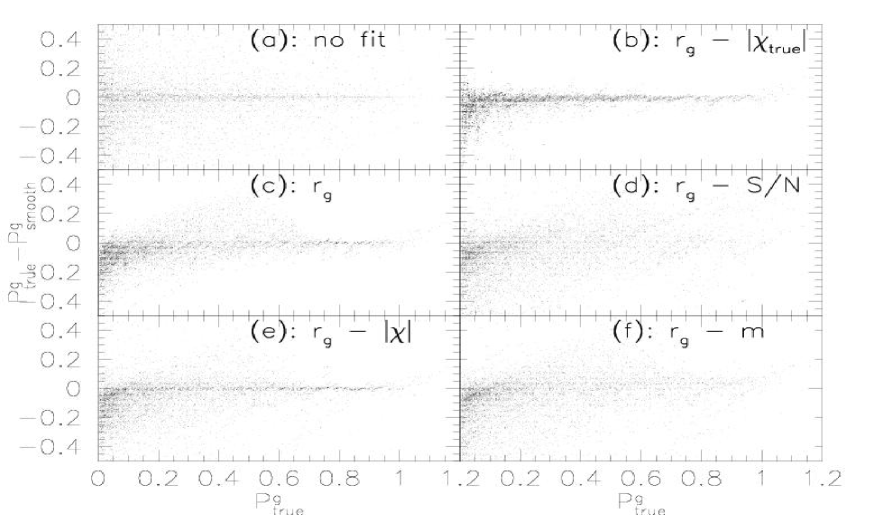
Fig. 2.: The difference between the true and smoothed $P^{\rm g}$ as function of $P^{\rm g}_{\rm true}$ with $P^{\rm g}_{\rm smooth}$ calculated in different parameter spaces. In panel (a) with no smoothing the errors of $P^{\rm g}$ are randomly distributed around the true value. In panel (c) (smoothing as function of $r_{\rm g}$) we see a systematic tail for intermediate values of $P^{\rm g}_{\rm true}$ indicating the dependence of $P^{\rm g}$ on at least one second parameter. Otherwise this smoothing reduces the noise very well. Panels (d) and (f) show that $P^{\rm g}$ does not depend on S/N or m. From panel (b) we see that $P^{\rm g}$ depends on the raw ellipticity $|\chi|$ as well as on $r_{\rm g}$. Unfortunately our measured, noisy ellipticities lead to significant noise in the smoothing [panel (e)].

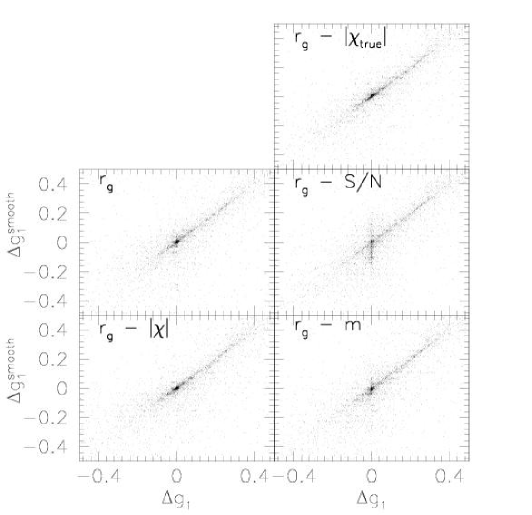
Fig. 3.: The errors $\Delta g_{1}:=g_{1}^{\rm true}-g_{1}$ vs. $\Delta g_{1}^{\rm smooth}:=g_{1}^{\rm true}-g_{1}^{\rm smooth}$ for the various smoothings of $P^{\rm g}$. Even for the best smoothing of this quantity with $r_{\rm g}$ and the true raw ellipticity $\chi_{\rm true}$ we have $\Delta g\approx\Delta g^{\rm smooth}$ indicating that smoothing $P^{\rm g}$ does not improve the shear estimation. The parameter spaces $r_{\rm g}$ and $r_{\rm g}-|\chi|$ give similar results while the $r_{\rm g}-$S/N smoothing especially shows a spread of $\Delta g_{1}^{\rm smooth}$ where $\Delta g_{1}=0$. The result implies that smoothing $P^{\rm g}$ does not improve the final shear estimate. We checked that this general result also applies for objects with an intrinsic, unphysical negative value for $P^{\rm g}$ (see text).

4.2 Weighting scheme

Similarly, we now search for the best possible parameter space to calculate $\sigma_{\rm g}^{2}$, and thus the weighting of the galaxy ellipticities. For this investigation we used a catalog with intrinsically round objects to isolate pixel noise errors from those of the intrinsic ellipticity distribution. The input shear is $g_{1}=0.03$, $g_{2}=0.0$. Fig. 4 shows that using $\pi_{U}=(r_{\rm g},{\rm m})$ and $\pi_{U}=(r_{\rm g},{\rm S/N})$ as parameter spaces for the $\sigma_{\rm g}^{2}$ calculation give the best and very comparable results in the final shear estimation. The errorbars in this and all following calculations are estimated by creating 200 bootstrap realisations of our catalog in the following way: We randomly take $N$ objects out of our catalog containing $N$ objects allowing for multiple entries. From this sample we recalculate a shear estimate and repeat the exercise $N_{\rm boot}=200$ times. From these shear estimates $g_{i}^{\rm boot};i\in[1..N_{\rm boot}]$ the errorbar for the original measurement is estimated by $\sigma_{\langle x\rangle}^{2}=\frac{1}{N_{\rm boot}}\sum_{i}(g_{i}^{\rm boot}-\langle g_{i}^{\rm boot}\rangle)^{2}$ (we checked that $\langle g_{i}^{\rm boot}\rangle$ is in excellent agreement with our original shear measurement). We note from Fig. 4 that introducing our weighting scheme improves the shear estimation significantly in comparison to no weighting. Therefore, weights from the $\pi_{U}=(r_{\rm g},{\rm S/N})$ smoothing are now used throughout.

Fig. 4.: The measured reduced shear $g_{1}$ as a function of the object size for various parameter spaces used in our weighting scheme. Panel (a) shows the result for noise free objects. Panels (b) and (c) show results if no weighting at all is applied, (d) and (e) for $r_{\rm g}$ and $r_{\rm g}-$m smoothings and finally (f) and (g) for the parameters $r_{\rm g}g-$S/N. The error bars are from 200 bootstrap realisations of the galaxy samples (see text). We note that the weighting scheme improves the measurement significantly to the cases where no weighting scheme is applied. We also conclude that there is no need to exclude low S/N objects from the measurement if weighting is applied.

4.3 Accuracy of shear estimates

To evaluate how accurately we can measure gravitational shear we have investigated the $g_{1}$, $g_{2}$ combinations listed in Table 1. We did our measurements first without PSF anisotropy and then with a stellar axis ratio $b_{*}/a_{*}=0.9$ with $a_{*}$ oriented such that $q_{2}^{*}=0$. To obtain the results quoted below, we have calculated averages $\langle{\bf{g}}\rangle$ and errors $\sigma_{\langle{\bf{g}}\rangle}$ over all galaxies in our catalogs. The results for the noise-free calculations are shown in Fig. 5. Note here that we have also used the same weighting scheme for the noise-free calculations, although this would not be necessary. From the plot we see the following trends for the calculations without PSF anisotropy:

• For small input shear values $|{\bf{g}}|\leq 0.1$ we can clearly recover the input shear within $\Delta{\bf{g}}\approx 0.01$ with the tensor as well as with the scalar shear estimator. For larger shear values we systematically underestimate the shear, with a maximal underestimation of $0.02$ to $0.03$ for the highest input shear of $0.2-0.25$. We note that for both shear estimators the underestimation as a function of input shear can be very well represented by a straight line indicating that the underestimation is a constant fraction of the input shear over the whole range of input shears considered here. This fraction is about $10\%-15\%$ for the scalar and $5\%-10\%$ for the tensor shear estimate.

• We also note that the results are completely equivalent in both shear components.

For the simulations with PSF anisotropy in the $g_{1}$ direction we conclude the following:

• Considering the $g_{2}$ component the results are very similar to the isotropic PSF case.

• For the $g_{1}$ component the scalar correction underestimates the shear by an amount comparable to the isotropic PSF case. In contrast, the tensor correction overestimates the input shear in the direction of the PSF anisotropy. This relative overestimate is about $20\%$ for the high $|{\bf{g}}|$ and can reach up to $100\%$ for the lowest input shears. In Fig. 8 we show analytic results with intrinsically round objects and an input shear of $g_{1}=0.25$. These calculations confirm that for Gaussian profiles the tensor correction overestimates the final shear in the direction of a PSF anisotropy. From our analysis of the SkyMaker simulations in Sect. 6, where we have encountered similar problems with the tensor correction, we conclude that the problems are not connected with the anisotropy correction of KSB but with the smearing correction.

Fig. 5.: The errors on shear recovery for noise-free objects. The crosses and filled hexagons show results for the scalar and tensor estimates with no PSF anisotropy present, the stars and filled pentagons for calculations with a $10\%$ PSF anisotropy in the $g_{1}$ direction. No object selection was done and our weighting scheme was used. The points were obtained by averaging over all $\approx 75000$ galaxies that we have for every shear realisation in our catalog. The error bars are less than 0.1 percent and so smaller than the symbols. For clarity of the plot the errorbars have been omitted and the symbols for the scalar correction have been slightly shifted to the right.

For the calculations including sky noise we have investigated the whole sample, and two sub-samples with S/N$<2$ and S/N$>2$. Fig. 6 shows that the S/N$>2$ sample results are similar to the noise-free case, i.e. in the absence of PSF anisotropy we have very good results with the tensor estimate (however, there is no underestimation in the tensor case at all in contrast to the noise-free case; in fact, the underestimation is lowered to $4\%$ in the noise-free case for the same subsample of galaxies), and about a $10\%-15\%$ underestimate for the scalar calculations. For the low signal-to-noise objects (S/N$<2$) the shear is underestimated by about $30\%$ in the scalar and up to about $50\%$ in the tensor case, where the underestimate in the tensor case shows an increasing trend for increasing shear. The error in the object centre determination is not the main reason for the underestimate: for S/N$<2$ we repeat the same calculations using the true object centres. The results from this test are very comparable to those shown here. For the whole sample, the scalar correction is better with a relative underestimate of about $10\%-15\%$ over the tensor one which has an underestimate of about $20\%-30\%$. If PSF anisotropy is present, noise-free and noisy cases give the same trends. Fig. 7 shows the noise amplitude of the estimators. We considered the ratio of the shear uncertainty from noisy objects $\sigma$ and the noise free calculations $\sigma^{\rm true}$. For S/N$>2$ pixel noise increases the errors in the shear estimates by about a factor of 2, for S/N$<2$, by a factor 5-10, and by a factor of 5 for the whole sample.

Fig. 6.: The same as Fig. 5 for noisy objects. The two upper most panels show results for S/N$>2.0$, the middle panels for S/N$<2.0$ and the lower panels for the whole sample. For high S/N objects, the tensor estimation is more accurate but in general the scalar calculation is much more stable towards low signal objects. Symbols for the scalar correction are slightly shifted to the right for clarity of the plot. For more details see the text.

Fig. 7.: The noise properties of the shear estimations from Fig. 6. For high S/N objects, sky noise only has a very weak contribution to the shear estimates. It increases the uncertainty by a factor 3-5 for low S/N objects and by a factor of about 2-3 for the whole sample. Symbols for the scalar correction are slightly shifted to the right for clarity of the plot. The panels are for the same object samples as in Fig. 6.

Fig. 8.: Analytical results for $g_{1}=0.25$, round intrinsic objects, no PSF anisotropy and a $10\%$ PSF anisotropy in the $g_{1}$ direction are shown. The solid and short dashed lines are scalar and tensor shear estimate for the PSF anisotropy free case, the long dashed and dashed dotted line represent scalar and tensor correction when PSF anisotropy is present. The figure confirms that the resulting shear is overestimated significantly in the tensor case with PSF anisotropy.

Fig. 9.: Results for Gaussian profiles put on FITS images and analysed with the procedure outlined in Sect. 5 are shown. Panels (a) and (b) are for the PSF anisotropy free case and the panels (c) and (d) for a PSF anisotropy of $10\%$ in the $g_{1}$ direction. All galaxies were used and no selection according to S/N was done. Dots with errorbars represent measurements with tensor estimation, lines with errorbars those with scalar estimation. The final estimates were done with about 13500 galaxies for every realisation and error bars have a typical size of $1\%$. The results are completely comparable to the S/N$>2$ case of Fig. 6

4.4 Summary

With our proposed way to apply the KSB technique to measure gravitational shear we come to the following conclusions when dealing with Gaussian profiles:

• Our analysis shows that the scalar estimator from eq. (8) systematically underestimates shear by about $10\%-15\%$. For low-S/N objects, the underestimate is about $30\%$. The tensor estimator from eq. (7) is better for high-S/N objects showing no systematic over- or underestimation in the final result. This estimator is less stable for low-S/N objects where there is a systematic underestimation that can reach more than $50\%$. When including PSF anisotropy, the scalar estimator still gives very stable and comparable results both in the direction of the PSF anisotropy and perpendicular to it. In contrast, we overestimate the shear in the direction of PSF anisotropy in the tensor case. We conclude that the scalar estimator is more stable and conservative. Both estimators show very similar noise properties.

• We have shown that smoothing $P^{\rm g}$ does not improve the final shear estimates over taking raw, noisy values.

• We can give an objective parameter cut S/N$>2$ for which we can measure shear with about the same accuracy as with no sky noise. Our S/N parameter [see eq.(17)] is very convenient as we do not have to find the threshold for every observation individually (as would be the case for quantities like m).

As a final step we have repeated the analysis done here putting our Gaussian galaxies and stars on FITS images and analysing them in the same way as the SkyMaker simulations described in the next section. In addition to the steps presented so far, we first have to perform object detection and selection for the shear determination. The steps for this are summarised below in Sect. 5. An important difference with the previous semi-analytical calculations is the fraction of S/N$<2$ objects. Previously they constituted more than $60\%$ of all the objects, but for the simulations where objects have to be detected first, this fraction is very small, about $5\%-10\%$ in the final catalogs. It turned out that shear estimates with the subsample S/N$>2$ and the complete sample are now similar, so that the small subsample of low-S/N objects becomes unimportant. Therefore, only the results with all objects without a cut in S/N will be shown from now on. Fig. 9 displays the results from the simulations. They are comparable to those obtained from the S/N$>2$ subsamples in Fig. 6. We also conclude that the stellar objects detected in the FITS images have sufficient signal to noise to give reliable estimates for $P^{\rm g}$. As described above we only used very high S/N stellar objects in the analytic calculations. This last simulation ensures that our shear analysis pipeline gives results consistent with analytical prediction, and that it is ready to be used for the final analysis involving the realistic simulations done with SkyMaker. In the next section, we first describe our procedure leading from the image frames to a galaxy catalog for shear measurements. Afterwards we will see whether our results are still valid when considering different galaxy profiles and especially more realistic PSFs.

5 Object detection and selection

In this section we describe a fully automatic procedure to go from image frames to a final object catalog for shear analysis. We note that our main intention was to obtain a catalog ensuring reliable measurements. We demonstrated at the end of the last section that our analysis of isolated objects in the semi-analytical treatment and with those detected in FITS images gives very comparable results. Our procedure contains several conservative rejection criteria for objects and it is not optimised to make the maximal use of data in terms of number density of objects. The procedure consists of the following steps:

Fig. 10.: The distribution of the positional differences of the ‘hfindpeaks’ position estimator and ours from eq. (16). We see a clear peak below 0.1 pixel and so we conservatively excluded all objects with a higher difference. See the text for more details.

1. Objects were detected with the ‘hfindpeaks’ algorithm from Nick Kaiser: The image is smoothed with Mexican top hat filters $W_{\rm d}(|\theta|)$

   $$W_{\rm d}(|\theta|)=\frac{1}{2r_{\rm g}^{2}\pi}\left[\exp\left(-\frac{|\theta|^{2}}{2r_{\rm g}^{2}}\right)-\frac{1}{r_{\rm f}^{2}}\exp\left(-\frac{|\theta|^{2}}{2r_{\rm f}^{2}r_{\rm g}^{2}}\right)\right]$$ (18)

   with increasing filter radii $r_{\rm g}$. In every smoothed image, the peaks are detected and linked with the peaks found in previous smoothings. Hereby peaks are assumed to belong to the same object if their positions coincide within $r_{\rm g}$. In this way a peak trajectory is built up for every potential object. For every peak, a signal-to-noise ratio $\nu$ is calculated where the signal is the peak value in the smoothed image and the noise $\sigma_{\rm d}$ is given by

   $$\sigma_{\rm d} = \sigma_{\rm sky}\sqrt{\int W_{\rm d}^{2}(\theta){\rm d}^{2}\theta}$$ (19)

   $$= \sigma_{\rm sky}\sqrt{\frac{1}{2\sqrt{\pi}r_{\rm g}}\left(1+\frac{1}{r_{\rm f}^{2}}-\frac{4}{1+r_{\rm f}^{2}}\right)},$$

   with $r_{\rm f}=2$. Fig. 11 shows a comparison between this signal-to-noise estimate and ours from eq. (17).

   

   Fig. 11.: A comparison between the ‘hfindpeaks’ signal-to-noise estimate $\nu$ and ours from eq. (17). The relation is a straight line and our criterion for a good object (S/N$>2$) corresponds to $\nu\approx 7$.

   Afterwards, peaks with the highest $\nu_{\rm max}$ value for each trajectory identify objects (peaks with $\nu_{\rm max}<4$ are immediately rejected). This size $r_{\rm g}$ is used in all the following analyses and the pixel centre of the peak position is taken as a starting point for the object centre determination. To get a more accurate object centre, a Newton-Raphson step is performed and the $x$ and $y$ pixel-positions are corrected from the pixel centre by $\delta_{x}$ and $\delta_{y}$

   $$\delta_{x}=-\frac{I_{x}^{s}}{I_{xx}^{s}};\;\;\;\delta_{y}=-\frac{I_{y}^{s}}{I_{yy}^{s}}$$ (20)

   where $I_{x}^{s}$, $I_{y}^{s}$ and $I_{xx}^{s}$, $I_{yy}^{s}$ are the first and second derivatives of the smoothed light profiles along $x$ and $y$.

2. From the peaks (objects) found in the previous step, all relevant quantities (like $P^{\rm sh}$, $P^{\rm sm}$) are calculated separately with the original, unsmoothed image.

3. From the catalog generated in the previous step, we first removed objects with obvious problems during the analysis process: (1) Objects closer than $3r_{\rm g}$ to the border of the image; (2) objects where one of the eigenvalues $A^{2}$, $B^{2}$ from the $Q_{ij}$ tensor was negative.

   $${A^{2}\choose B^{2}}=\frac{Q_{11}+Q_{22}}{2}{+\choose-}\sqrt{\left(\frac{Q_{11}-Q_{22}}{2}\right)^{2}+4Q_{12}^{2}};$$ (21)

   (3) the object has a total negative flux. (4) Fig. 10 shows the distribution of the difference between the centroid estimates of ‘hfindpeaks’ and ours from eq. (16). All objects with a difference larger than 0.1 pixel were excluded. We found that this is an efficient way to reject blended objects, since one centroid estimator is based on the smoothed and the other on the unsmoothed image.

4. Objects with a neighbour within $3r_{\rm g}$ are rejected.

5. Stars are preselected using the star branch of the $r_{\rm h}-$m diagram and polynomials for the two components of ${\bf{q}}^{*}$ are calculated in the following way: a preliminary fit is done for $q^{*}_{1}$ and $q^{*}_{2}$ using a $\chi^{2}$ minimisation

   $$\chi^{2}_{j}=\sum_{i=1}^{N^{*}}(q^{*}_{j}(x_{i},y_{i})-p_{j}(a_{k},x_{i},y_{i}))^{2},$$ (22)

   where $N^{*}$ is the number of preselected stars, $j=1,2$, $x_{i},y_{i}$ are the positions of the stars and $p_{j}$ are two-dimensional, second order polynomials with six unknown parameters $a_{k}$. After determination of $a_{k}$ we calculated the expected error $\sigma_{q_{j}}$ for every $q^{*}_{j}$ by

   $$\sigma_{q^{*}_{j}}=\sqrt{\frac{{\chi^{2}_{j}}_{\rm min}}{N^{*}-1}},$$ (23)

   where ${\chi^{2}_{j}}_{\rm min}$ is the minimum of $\chi^{2}_{j}$ at the fitted parameters $a_{k}$. Stars which deviate at more than $1\sigma_{q_{j}}$ in any of the two components $q_{1}$ or $q_{2}$ are rejected, and the fit is repeated for the final polynomials.

6. The final sample of stars is reprocessed nine times with filter scales $r_{i}=1..9$, in order to match all the possible galaxy sizes. After each processing, objects with problems according to step (21) are still rejected. From the remaining stars we calculated the mean of $\langle{\rm tr}[P^{*\rm sh}]/{\rm tr}[P^{*\rm sm}]\rangle$ and we used this value for the PSF correction.

7. We now have all the quantities in hand to calculate scalar and tensor shear estimates for every objects as described in Sect. 2.1. Hereby we considered only objects as galaxies whose half light radius was larger than the stellar locus (see Fig. 1).

8. Weights for the tensor and scalar ${\bf{g}}$ are calculated, which is an important ingredient for the two shear estimators as described in Sect. 2.1. With the whole procedure we end up with a number density of about 30 galaxies per sq. arcmin.

6 The SkyMaker simulations

Fig. 12.: A comparison of galaxy properties in one of our SkyMaker images with real data in one of our $I$ band CFHT fields. Both images had a seeing of $0{\hbox{$.\!\!^{\prime\prime}$}}7$ and both corresponded to 12000 sec. exposures. Objects have been detected and the quantities have been calculated with SExtractor. The two upper panels show a comparison of the magnitude distribution, the two middle panels of the object size defined as $\sqrt{AB}$, where $A$ and $B$ are defined as in eq. (21) and the lower panels of the ellipticity parameter $\epsilon=(1-B/A)/(1+B/A)$. The only noticeable strong difference is that the ellipticity distribution in the real data is slightly broader. The shift of the peak in this distribution is caused by a strong PSF anisotropy in the CFHT data.

6.1 The image characteristics of our SkyMaker simulations

For every combination of the shear and PSF, ten SkyMaker images were produced and analysed. Each image has the characteristics of a 12000 sec. $I$ band exposure taken at a telescope with a 3.5m primary and a 1m secondary mirror, and has a dimension of $2048\times 2048$ pixels with a scale of 0$.\!\!^{\prime\prime}$206 per pixel. The atmospheric seeing in every image was 0$.\!\!^{\prime\prime}$7. For every image we detected our objects and analysed them as described above. A comparison of magnitude distribution, object size and ellipticity distribution between detected objects in one of the images and a 12000 sec. $I$ band CFHT image having a measured seeing of 0$.\!\!^{\prime\prime}$7 is shown in Fig. 12. A description how the PSF is constructed in SkyMaker is given in the Appendix.

6.2 Results of the SkyMaker simulations

Fig. 13 shows contours of the outer and core parts of the PSFs we have used in our simulations. The outer parts of the profiles all look the same (except for the quadratic PSF) and they differ mostly in the cores. The anisotropies caused by these PSFs are given in Table 2.

	PSF_1	PSF_2	PSF_3	PSF_4
$\chi_{1}$	0.00	0.00	0.00	0.00
$\chi_{2}$	0.00	0.01	0.00	0.00

	PSF_5	PSF_6	PSF_7	PSF_8
$\chi_{1}$	0.1	0.06	0.04	0.00
$\chi_{2}$	0.07	0.03	-0.03	0.00

Table 2.: The anisotropies of the PSFs described in Fig. 13. The values quoted are the raw ellipticity measurements from KSB where the $r_{\rm g}$ from the stars was used as filter scale.

For every PSF we have analysed seven sets of images with the shear combinations given in Table 3 where a few sets are slightly different from those in Table 1.

$g_{1}$	0.01	0.03	0.25	0.08	0.2	0.2	0.14
$g_{2}$	0.007	0.05	0.2	0.14	0.27	0.14	0.2

Table 3.: The shear combinations we investigated with our SkyMaker simulations.

The results for our SkyMaker simulations are shown in Figs. 14, 15, 16 and Table 4. As for the semi-analytical and simulated Gaussian profiles we now discuss the accuracy of the shear estimators for the different shear amplitudes and PSF anisotropies:

• In the case of no PSF anisotropy at all (PSF_1), the tensor correction gives the correct shear on the whole range of $|{\bf{g}}|=0.012$ up to $|{\bf{g}}|=0.32$. The scalar correction underestimates the shear relatively by about $10\%-15\%$. The $1\sigma$ error bars are about at $\pm 0.005$.

• In the presence of PSF anisotropy, the tensor correction can over- or underestimate the true shear while it is always underestimated in the scalar case. In the sense of deviation from the true value, the tensor case always gives the better result. The relative underestimates with the scalar correction can reach up to $30\%$ in the worst case. As the anisotropy of stars is perfectly corrected by our polynomials for $p$, we investigated whether there is nevertheless an anisotropy residual in the galaxies. For this we compared the position angle from the input shear with the recovered one in Fig. 16. There we see that in the scalar case the position angle is nearly perfectly recovered. This means that the PSF anisotropy is corrected very well but the calibration factor $P^{\rm g}$ is too low. In the tensor case the recovery of the position angle is not as good as in the scalar case but also very acceptable. The reason for the over- or underestimates of the magnitude of the shear is probably that the elements of $P^{\rm g}$ that are used for the isotropic correction should be calculated from profiles that are already corrected for PSF anisotropy defects.

• From Table 4 we conclude that also for all the SkyMaker simulations, the over- or underestimates are nearly a constant fraction of the input shear. For the tensor estimator we can typically recover the input shear to an accuracy between $10\%-15\%$. This means that we can measure a shear below $0.1$ nearly within $0.01$, the accuracy required for accurate measurements of the cosmic shear on scales $\leq 10{\hbox{$.\!\!^{\prime}$}}0$.

• For all the SkyMaker simulations the recovery of the shear is better than in the anisotropic case with Gaussian profiles (see Fig. 9). It seems that the more realistic SkyMaker PSF profiles better reflect the assumptions in the KSB algorithm than Gaussian profiles, namely that PSF anisotropy mainly comes from the central core. While a Gaussian has its anisotropy on all scales, Fig. 13 shows that the anisotropy details of the SkyMaker PSFs lie in the core indeed.

• Regarding the issue of scalar vs. tensor correction, we can conclude that, although the scalar case always underestimates the true shear, it provides the more conservative answer and it should be used when one is interested mainly in the position angle of objects while the tensor should given preference when the amplitude of the shear is important.

7 Conclusions and Outlook

In this paper we have investigated how well we can recover weak gravitational shear with realistic simulations for ground-based observations. With respect to the main motivation for this work, to test the reliability of our recent detection of cosmic shear, the results are very encouraging. In all our simulations we could recover weak shear up to $|{\bf{g}}|=0.1$ with an accuracy of $0.01$ or better and we can significantly exclude the detection of a $|{\mbox{\boldmath$\gamma$}}|=0.04-0.05$ false signal based purely on uncorrected PSF effects. Although the PSFs we have investigated do certainly not cover all possible defects mimicking a lens signal, also other independent studies like Hoekstra et al. (1998), who looked at diffraction-limited model PSFs for the HST or Bacon et al. (2000b), indicate that the KSB algorithm works better than one could expect looking at its assumptions. We showed that for the PSFs investigated here, the anisotropy correction proposed in the original KSB work is working very well, but that there are problems with the isotropy correction if an anisotropy is present. The reason for this is probably that in such a case, the boost factor $P^{\rm g}$ is calculated with the wrong, not anisotropy-corrected, galaxy profile. Moreover, we have presented a fully automatic procedure leading from the image frames to an object catalog for reliable shear measurements. Despite these encouraging results, the advent of new wide-field imaging mosaic cameras in particular, and the associated data flow brings additional technical problems if we want to build up a fully automatic data processing pipeline. Some of these problems that we could not address in the scope of this work, but leave to a future publication are:

1. In wide-field imaging especially, many images suffer from very bright stars causing blooming effects, strong stray light and reflections. So far, we usually have marked out affected image regions by hand, but it should be investigated whether there are automatic ways of dealing with it.

2. We usually coadd several single exposures to get a final image. These frames typically have slightly different seeing disks. In the past we often simply did not use images that had the worst seeing. We have to investigate what effects the coaddition of images with different PSF properties has on the final shear measurement result.

3. As a consequence of the last point, weak-lensing observations have mostly been done with a very compact dither pattern so far. This has the advantage of allowing a simple coaddition of the images with integer pixel shifts, and the effects of optical image distortions do not need to be taken into account during the image prereduction. This first preserves uncorrelated noise in the image pixels, second it preserves the smoothness of PSF anisotropy on the scale of single chips, and third it brings the practical advantage that we can still deal with single chips instead of very large images. Nevertheless, we think that this approach is not ideal. On the one hand accurate astrometry and photometry is done most easily if information from objects in the overlap between different chips is at hand. The afore mentioned advantages may turn into problems in later analysis when the gaps between single chips lead to severe border effects, e.g. when we try to search for filaments between galaxy clusters (see Kaiser et al. 1999). So we will investigate whether we can overcome the effects of correlated pixel noise caused by remapping for optical distortions and discontinuities of the PSF anisotropy in the final coadded images.

Fig. 13.: The figure shows the outer part (left) and the core (right) of the PSFs used in the SkyMaker simulations. All the PSFs contain four spider arms produced by the support of the secondary mirror. From left to right and from bottom to top the PSFs contain the defects (For the tracking errors, the first value in the bracket gives the rms drift in the direction of the second value. The third value is the rms of a Jitter in the orthogonal direction. For the aberrations the “d80” diameters introduced are quoted (see the appendix for a detailed description of tracking errors and aberrations). We note that the “d80” diameters of the individual aberrations do not add quadratically as the aberration polynomials are not orthogonal.): (1) None; (2) tracking error (0.0”, 97.0^∘, 0.05”), defocusing (0.05”), coma (0.26”); (3) tracking error (0.05”, 0.0^∘, 0.01”), defocusing (0.07”) and triangular aberration (0.015”); (4) tracking error (0.02”, 34.0^∘, 0.02”), defocusing (0.1”) and spherical aberration (0.3”); (5) tracking error (0.3”, 31.0^∘, 0.2”), defocusing (0.3”) and astigmatism (0.72”); (6) tracking error (0.3”, 62.0^∘, 0.3”), defocusing (0.3”), coma (0.31”) and triangular aberration (0.72”); (7) tracking error (0.5”, -20.0^∘, 0.11”), defocusing (0.07”) and triangular aberration (0.122”) (8) defocusing (0.05”) and quadratic aberration (0.61”)

Fig. 14.: From top to bottom the figure shows SkyMaker results for the first four PSFs of Fig. 13. The objects from the ten images for every shear/PSF combination were pasted together and the means and errorbars shown here were obtained from this pasted catalog.

Fig. 15.: The same as Fig. 14 for the second four PSFs of Fig. 13.

Fig. 16.: The figure shows the difference ($\theta^{\rm true}-\theta$) of the recovered position angles vs. the position angles of the input shear. Crosses correspond to the results from Fig. 14 and diamonds to those from Fig. 15. Triangles are for shear values where no PSF anisotropy correction has been done (PSF_4). In this plot we omitted the very weak shear case ($g_{1}=0.01$, $g_{2}=0.007$) as the position angle is badly determined here.

Results of the SkyMaker simulations
	$g_{1}$	$g_{2}$	$g_{1}$	$g_{2}$	$g_{1}$	$g_{2}$	$g_{1}$	$g_{2}$	$g_{1}$	$g_{2}$	$g_{1}$	$g_{2}$	$g_{1}$	$g_{2}$	objects	$r_{h}$
input shear	0.01	0.007	0.03	0.05	0.25	0.2	0.08	0.14	0.2	0.27	0.2	0.14	0.14	0.2	per $(1\hbox{${}^{\prime}$})^{2}$	(stars)
PSF_1 scalar	-52.93	7.41	-26.20	-20.56	-13.79	-17.44	-12.03	-15.82	-14.31	-15.92	-15.66	-13.41	-13.78	-16.01
PSF_1 tensor	-68.73	47.70	-13.98	-16.13	-0.67	0.70	-0.97	-9.03	5.72	-1.69	-5.75	-0.51	-2.61	-6.56	40	$\approx 1.95$
PSF_2 scalar	11.39	-46.60	-18.62	-14.96	-14.01	-14.08	-13.10	-16.95	-13.77	-15.09	-12.50	-14.68	-15.36	-16.98
PSF_2 tensor	33.70	8.63	-26.04	-9.70	4.09	5.94	-2.51	-2.47	7.09	7.23	1.36	1.08	-4.08	0.65	28	$\approx 2.15$
PSF_3 scalar	-20.31	-18.57	-16.40	-10.96	-20.50	-24.39	-22.80	-24.55	-22.43	-23.62	-19.42	-22.81	-18.19	-23.21
PSF_3 tensor	-21.30	-10.27	-18.62	2.43	-10.20	-12.95	-15.13	-13.14	-11.52	-9.69	-11.01	-11.09	-9.80	-10.78	35	$\approx 1.95$
PSF_4 scalar	-16.54	3.09	-32.02	-25.30	-22.12	-23.36	-18.46	-22.62	-20.34	-23.12	-22.56	-22.94	-22.48	-23.59
PSF_4 tensor	-18.59	-18.81	-22.81	-18.60	-9.97	-10.03	-14.99	-13.55	-8.63	-10.18	-15.84	-11.43	-17.88	-14.02	33	$\approx 2.05$
PSF_5 scalar	-121.00	-55.93	-13.59	-20.69	-20.11	-24.76	-23.08	-21.41	-17.98	-21.92	-17.73	-23.75	-21.24	-22.06
PSF_5 tensor	21.60	25.20	14.79	-5.56	1.54	-1.89	1.95	-10.15	11.45	2.29	6.21	6.18	3.36	-5.98	21	$\approx 2.75$
PSF_6 scalar	0.20	-35.93	-1.00	-16.40	-27.17	-25.75	-27.62	-24.74	-27.76	-23.07	-23.80	-29.63	-21.22	-28.54
PSF_6 tensor	68.21	-37.49	19.49	-15.74	-9.36	-9.60	-0.57	-10.46	-7.10	-14.53	-8.41	-14.44	-3.47	-13.71	20	$\approx 3.05$
PSF_7 scalar	-31.28	-20.51	-11.07	-19.00	-24.77	-23.41	-20.16	-25.42	-25.79	-26.21	-23.81	-24.70	-22.89	-22.43
PSF_7 tensor	-2.78	-47.23	2.29	-15.14	-12.80	-13.94	-6.62	-20.22	-12.74	-17.98	-14.60	-18.66	-10.03	-15.06	32	$\approx 2.25$
PSF_8 scalar	-17.09	-33.79	-19.97	-30.31	-23.48	-26.78	-27.67	-27.56	-24.14	-27.00	-23.77	-25.73	-26.45	-27.02
PSF_8 tensor	-24.40	-33.53	-14.92	-25.71	-10.36	-16.04	-20.36	-22.62	-13.71	-17.06	-13.57	-14.93	-16.15	-19.44	30	$\approx 2.25$

Table 4.: The table gives a summary of the results from the SkyMaker simulations performed. Given is the relative error $(g_{1,2}-g_{1,2}^{\rm true})/g_{1,2}^{\rm true}$ in percent. We note that this error is always a fairly constant fraction over the whole range of input shears (excluding the very weak shear case). The mean number of used objects per sq. arcmin and the measured stellar $r_{h}$ are from the catalogs of the $g_{1}=0.01$, $g_{2}=0.007$ input shear.

Appendix: The SkyMaker program

SkyMaker is an image simulation program, a kind of “virtual telescope” originally designed to assess SExtractor detection and measurement performances (Bertin & Arnouts 1996). The code (Version 2.3.3) has been much improved since, and is currently capable of simulating star and galaxy images with higher accuracy.

The optical Point Spread Function (PSF)

Simulated images feature a PSF which is assumed to be the convolution of the telescopic (instrumental) point-spread function, tracking errors, and atmospheric “seeing” (assuming a long exposure time). We shall however more conveniently deal with the Optical Transfer Function (OTF), which is just the Fourier transform of the PSF.

Telescope

Although the diffraction spot of a large telescope is small compared to the atmospheric seeing disk at optical wavelengths, features such as diffraction spikes (created by the spider-arms of the secondary mirror/primary focus) are obvious on real images and must be taken into account.

The principle of the PSF generation is similar to that of other telescope image simulators like TIM (Hasan & Burrows 1995). The system is assumed to be illuminated with incoherent, quasi-monochromatic planar waves. In those conditions, the instrumental OTF is proportional to the autocorrelation of the input pupil function of the system (e.g. Born & Wolf 1999). The on-axis pupil function $P(\rho,\theta)$ used in this work is shown in Fig. 17. It is typical of telescopes like the 3.6m CFHT, harbouring wide-field instruments used for weak-lensing experiments.

Instead of using ray-tracing techniques to simulate off-axis aberrations, we preferred to approximate the latter by modulating the phase $\phi$ of the complex on-axis input pupil (as shown in Fig. 17). Aberrations are limited to the sum of low-order Seidel (1856) terms: defocus $\phi_{d}\propto\rho^{2}$; astigmatism $\phi_{a}\propto\rho^{2}\cos^{2}(\theta-\theta_{a})$; coma $\phi_{c}\propto\rho^{3}\cos(\theta-\theta_{c})$; spherical $\phi_{s}\propto\rho^{4}$; plus the triangular and quadratic aberrations. Each term is normalised in “d80” units, that is, the diameter of the disk within which 80% of the light from a point source image is enclosed, omitting the contribution from diffraction and other aberration terms (Fouqué and Moliton 1996, private communication).

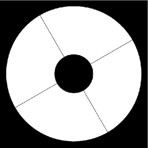
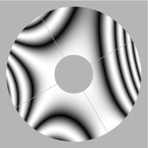
Fig. 17.: The input pupil used for the simulations. Note the secondary-mirror/primary-focus obstruction and the position angle of its support arbitrarily set to 30 deg. with respect to image axes. Left: Pupil function modulus. Right: Real part of the pupil function in presence of defocusing, coma and triangular aberrations (PSF_6 from Fig. 13).

Tracking errors

A tracking drift of angle $d$ in the $\theta_{T}$ direction can be simulated by multiplying the OTF by ${\rm sinc}\,(df).\delta(\theta-\theta_{T})$, where $f$ is the angular frequency. “Jittering” effects are easily added by multiplying the OTF by a centered, 2D Gaussian window.

Atmospheric turbulence

Close to zenith, atmospheric turbulence blurs long-exposure images in an isotropic way. Experimentally, the “atmospheric” OTF is found to quite accurately follow the theoretical prediction $\propto\exp-3.442\left(\frac{\lambda f}{r_{0}}\right)^{-5/3}$ for a turbulent atmosphere that follows Kolmogorov statistics (see for instance Roddier 1981 and references therein, or more recently Racine 1996). Fried’s (1966) $r_{0}$ parameter can be more conveniently expressed as a function of the “atmospheric” Full-Width at Half-Maximum and the wavelength $\lambda$: $r_{0}\approx 0.976\frac{\lambda}{\rm FWHM}$. There is no simple analytical expression for the resulting PSF, and although the core bears some resemblance to a Gaussian, the wings are significantly larger. The atmospheric FWHM varies only slowly with wavelength ($r_{0}\propto\lambda^{6/5}$, i.e. ${\rm FWHM}\propto\lambda^{-1/5}$). This results in a negligible dependency of star profiles on their spectral characteristics under ground-based standard broadband observing conditions: something essential for weak-lensing calibration, as stressed by Kaiser (1999).

The Aureole

A so-called “aureole” is observed to dominate all optical instrumental PSFs out to distances a few times the FWHM away from the centre. This is a feature which must be taken into account when simulating deep and wide galaxy fields, as it reproduces the background variations found on real images around bright stars. Although several sources contribute to the presence of the PSF aureole (light scattering caused by aerosols, dust on optics, scratches and micro-ripples on optical surfaces, see for instance Beckers 1995), it is experimentally found to follow quite a “universal” $r^{-2}$ profile (King, 1971). The intensity appears fairly constant too, being close to 16th mag per sq.arcsec for a 0th magnitude star. We adopted this value here.

Pixel footprint

Finally, the generously sampled (${\rm FWHM}\approx 40$ samples) instrumental+atmospheric PSF is convolved with the square pixel footprint (0.206”, like the CFH12K camera) and ready to be interpolated over the final image grid.

Simulated stars

Stars are simulated within SkyMaker, assuming a constant slope of the logarithm of differential number counts of 0.3 per magnitude interval, and a total sky density of 42000 per sq.degree down to $I$=25. The fairly high slope provides a crude match to star counts around $I$=20-21 at high galactic latitude (e.g. Nonino et al. 1999), while reducing the density of brighter stars.

Simulated galaxies

SkyMaker galaxies are made of a bulge with an $\exp r^{-1/4}$ profile and an exponential disk. All galaxy parameters are provided by the Stuff program as described in Sect. 3. Obviously, a study of weak-shear systematics requires accurate profiles, which means that simulated galaxies must be well sampled. Except for the most extended ones, the sampling step is that of the PSF (a few mas). Prior to convolution by the PSF, appropriate thresholding is applied to the wings of the composite galaxy profile to remove any “boxy” limit that may affect shear measurements.

Final image

A uniform sky background with surface brightness $\mu_{I}=19.9$mag.arcsec^-2 is added to the image. Surface brightnesses are then converted to ADUs assuming the image is the average of twelve 600s CFH12K exposures, yielding a magnitude zero-point of 32.6 mag and an equivalent conversion factor of 36 e^-/ADU. Poissonian photon white noise and Gaussian read-out white noise realisations are eventually applied. It is important to note that the simulation procedure skips three important steps, present in the reduction of real images: field warping, image resampling and co-addition. These points can have a significant impact on weak-shear measurements and will be addressed in a future paper.

References

- 1 Bacon D., Refregier A., Ellis R., 2000a, sumbitted to MNRAS (astro-ph/0003008)
- 2 Bacon D., Refregier A., Clowe D., Ellis R., 2000b, sumbitted to MNRAS (astro-ph/0007023)
- 3 Bartelmann M., Schneider P., 2000, Phys. Reports, in press (astro-ph/9912508)
- 4 Beckers J., 1995, Scientific and Engineering Frontiers for 8-10m Telescopes, eds M. Iye & T. Nishimura, 303
- 5 Bertin E., Arnouts S., 1996, A&A 117, 393
- 6 Binggeli B., Sandage A., Tarenghi M., 1984, AJ 89, 64
- 7 Brainerd T., Blandford R., Smail I., 1995, ApJ 466, 623
- 8 Clowe D., Kaiser N., Luppino G., Henry J.P., Gioia I.M., 1998, ApJ 497, L61
- 9 Erben T., van Waerbeke L. Mellier Y., et al., 2000, A&A 355, 23
- 10 Fischer P., et al., 1999, submitted to AJ (astro-ph/9912119)
- 11 Fried D.L., 1966, J. Opt. Soc. Am. 56, 1372
- 12 Hasan H., Burrows C.J., 1995, PASP 107, 289
- 13 Hoekstra H., Franx M., Kujiken K., Squires G., 1998, ApJ 504, 636
- 14 Hoekstra H., Franx M., Kujiken K., 2000, ApJ 532, 88
- 15 Hudson M., Gwyn S. D. J., Dahle H., Kaiser N., 2000, ApJ 503, 531
- 16 de Jong R.S., Lacey C., 1999, The Low Surface Brightness Universe, ASP Conference Series 170, 52
- 17 Kaiser N., 1999, (astro-ph/9904003)
- 18 Kaiser N., Squires G., 1993, ApJ 404, 441
- 19 Kaiser N., Squires G., Broadhurst T., 1995, ApJ 449, 460
- 20 Kaiser N., Wilson G., Luppino G., Dahle H., 1999, submitted to PASP (astro-ph/9907229)
- 21 Kaiser N., Wilson G., Luppino G., 2000, submitted to ApJ Lett. (astro-ph/0003338)
- 22 King I.R., 1971, PASP 83, 199
- 23 Kuijken K., 1999, A&A, 352, 355
- 24 Luppino G. A., Kaiser N., 1997, ApJ 475, 20
- 25 Natarajan P., Kneib J. P., Smail I., Ellis R., 1998, ApJ 499, 600
- 26 Nonino M, Bertin E., da Costa L., et al., 1999, A&AS 137, 51
- 27 Racine R., 1996, PASP 108, 699
- 28 Roddier F., 1981, Progress in Optics 19, 281
- 29 Schechter P., 1976, ApJ 203, 297
- 30 Schneider P., Rix H., 1997, ApJ 474, 25
- 31 Schneider P., van Waerbeke L., Mellier Y., et al., 1998a A&A 333, 767
- 32 Schneider P., van Waerbeke L., Jain B., Kruse G., 1998b, MNRAS 296, 873-892
- 33 Seidel L., 1856, Astr. Nachr. 1027, 289
- 34 Tyson J. A., Valdes F., Wenk R. A., 1990, APJ 349, L1
- 35 Umetsu K., Futamase T., 2000, submitted to ApJ Lett. (astro-ph/0004373)
- 36 Van Waerbeke L., Mellier Y., Erben T., et al., 2000, A&A 358, 30
- 37 Wittman D. M., Tyson J. A., Kirkman D., Dell’Antonio I., Bernstein G., 2000, Nature 405, 143