Power Spectrum Analysis of the ESP Galaxy Redshift Survey

Abstract

We measure the power spectrum of the galaxy distribution in the ESO Slice Project (ESP) galaxy redshift survey. We develope a technique to describe the survey window function analytically, and then deconvolve it from the measured power spectrum using a variant of the Lucy method. We test the whole deconvolution procedure on ESP mock catalogues drawn from large N–body simulations, and find that it is reliable for recovering the correct amplitude and shape of $P(k)$ at $k>0.065\,h$ Mpc^-1. In general, the technique is applicable to any survey composed by a collection of circular fields with arbitrary pattern on the sky, as typical of surveys based on fibre spectrographs. The estimated power spectrum has a well–defined power–law shape $k^{n}$ with $n\simeq-2.2$ for $k\geq 0.2\,h$ Mpc^-1, and a smooth bend to a flatter shape ($n\simeq-1.6$) for smaller $k$’s. The smallest wavenumber, where a meaningful reconstruction can be performed ($k\sim 0.06\,h$ Mpc^-1), does not allow us to explore the range of scales where other power spectra seem to show a flattening and hints for a turnover. We also find, by direct comparison of the Fourier transforms, that the estimate of the two–point correlation function $\xi(s)$ is much less sensitive to the effect of a problematic window function as that of the ESP, than the power spectrum. Comparison to other surveys shows an excellent agreement with estimates from blue–selected surveys. In particular, the ESP power spectrum is virtually indistinguishable from that of the Durham-UKST survey over the common range of $k$’s, an indirect confirmation of the quality of the deconvolution technique applied.

1 Introduction

The quantitative characterisation of the galaxy distribution is a major aim in the study of the large-scale structure of the Universe. During the last 20 years, several surveys of galaxy redshifts have shown that galaxies are grouped in clusters and superclusters, drawing structures surrounding large voids (see e.g. Guzzo 1999 for a review). The power spectrum of the galaxy distribution provides a concise statistical description of the observed clustering that, under some assumptions on its relation to the mass distribution, represents an important test for different structure formation scenarios (e.g. Peacock 1997 and references therein). Indeed, under the assumption of Gaussian fluctuations, the power spectrum totally describes the statistical properties of the matter density field (e.g. Peebles 1980).

In recent years, several estimates of the galaxy power spectrum have been obtained using galaxy samples selected at different wavelenghts: radio (Peacock & Nicholson 1991), infrared (Feldman, Kaiser & Peacock 1994, Fisher et al. 1993, Sutherland et al. 1999) and optical (Park et al. 1994, da Costa et al. 1994, Tadros & Efstathiou 1996, Lin et al. 1996, Hoyle et al. 1999), to mention the most recent ones.

The ESO Slice Project redshift survey (ESP, Vettolani et al. 1997, 1998) is one of the two deepest wide–angle surveys currently available, inferior only to the larger Las Campanas Redshift Survey (LCRS, Shectman et al. 1996). During the last few years, it has produced a number of statistical results on the properties of optically–selected galaxies, as e.g. the luminosity function (Zucca et al. 1997) or the correlation function (Guzzo et al. 2000). The geometry of the survey (a thin row of circular fields, resulting in an essentially 2D slice in space) is such that an estimate of the power spectrum represents a true challenge. In this paper we present the results of a detailed analysis that overcomes these difficulties, producing a reliable measure of the power spectrum from the ESP redshift data. The technique developed here to cope with the specific geometry of the survey is potentially interesting also for application to other surveys consisting of separate patches on the sky, as could be the case, for example, of preliminary sub–samples of the ongoing SDSS (Margon 1998) and 2dF (Colless 1998) surveys.

The outline of the paper is as follows. We shall first recall the main features of the ESP survey and the sample selection (section 2), then discuss the power spectrum estimator adopted for the analysis (section 3) and the numerical tests performed in order to check its validity range (section 4). We shall then present the estimated power spectrum (section 5) and its consistency with the correlation function (section 6), and then discuss it in comparison to the results from other surveys (section 7). Section 8 summarises the results obtained, drawing some conclusions.

2 The ESO Slice Project

The ESO Slice Project galaxy redshift survey (ESP, Vettolani et al. 1997, 1998) was constructed between 1993 and 1996 to fill the gap that existed at the time between shallow, wide angle surveys as the CfA2, and very deep, one-dimensional pencil beams. The survey was designed in order to allow the sampling of volumes larger than the maximum sizes of known structures and an unbiased estimate of the luminosity function of field galaxies to very faint absolute magnitudes. The survey and the data catalogue are described in detail in Vettolani et al. (1997, 1998). Here we limit ourselves to a summary of the main features relevant for the present analysis.
The ESP survey (see Figures 1 and 2) extends over a strip of $\alpha\times\delta=22\degr\times 1^{\rm o}$, plus a nearby area of $5\degr\times 1\degr$, five degrees west of the main

Figure 1: The area covered by the ESP survey on the sky consists of a set of 107 circular fields of $16^{\prime}$ radius. As shown in this figure, they are arranged into 2 parallel rows and draw two thin slices over the celestial sphere of about $22\degr\times 1\degr$ and $5\degr\times 1\degr$ respectively, separated by $\sim 5\degr$ (from Vettolani et al. 1997).

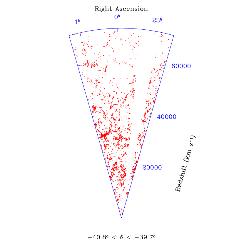
Figure 2: The galaxy distribution in the ESP redshift survey.

strip, in the South Galactic Pole region ($22^{h}30^{m}\leq\alpha\leq 01^{h}20^{m}$, at a mean declination of $-40^{\rm o}15^{\prime}$ (1950)). This region was covered with a regular grid of adjacent circular fields, with a diameter of 32 arcmin each, corresponding to the field of view of the multifibre spectrograph OPTOPUS (Avila et al. 1989) at the ESO 3.6 m telescope. The total solid angle covered by the survey is 23.2 square degrees and its position on the sky was chosen in order to minimize galactic absorption ($-75^{\rm o}\la b^{II}\la-60^{\rm o}$). The target objects, with a limiting magnitude $b_{J}\leq 19.4$, were selected from the Edinburgh–Durham Southern Galaxy Catalogue (EDSGC, Heydon–Dumbleton et al. 1989). A total of 4044 objects were observed, corresponding to $\sim 90\%$ of the parent photometric sample and selected to be a random subset of the total catalogue with respect to both magnitude and surface brightness. The total number of confirmed galaxies with reliable redshift measurement is 3342, while 493 objects turned out to be stars and 1 object is a quasar at redshift $z\sim 1.174$. No redshift measurement could be obtained for the remaining 208 spectra. As discussed in Vettolani et al. (1998), the magnitude distribution of the missed galaxies is consistent with a random extraction of the parent population. About half of the ESP galaxies present spectra with emission lines. Particular attention was paid to the redshift quality and several checks were applied to the data, using 1) multiple observations of $\sim 200$ galaxies, 2) $\sim 750$ galaxies for which the redshift from both absorption and emission line is available (Vettolani et al. 1998, Cappi et al. 1998). More details about the data reduction and sample completeness are reported in Vettolani et al. (1997, 1998).

Given the magnitude–limited nature of the survey, the computation of a clustering statistics like the power spectrum requires the knowledge of the selection function. This is defined as the expected probability to detect a galaxy at a redshift $z$ and can be expressed as

$$s(z)={\int_{{\rm max}[L_{1},L_{\rm min}(z)]}^{+\infty}\phi(L)dL\over\int_{L_{1}}^{+\infty}\phi(L)dL},$$ (1)

where $\phi(L)$ is the luminosity function, $L_{1}$ is the minimum luminosity of the sample and $L_{\rm min}(z)$ is the minimum luminosity detectable at redshift $z$, given the sample limiting magnitude.

In the ESP survey the minimum luminosity corresponds to an absolute magnitude $M_{b_{J},1}=-12.4+5\,\log h$ ($h$ is the Hubble constant in units of $100\,{\mathrm{k}m\,s}^{-1}{\mathrm{M}pc}^{-1}$). $L_{\rm min}(z)$ is the luminosity of a galaxy at redshift $z$ with an apparent magnitude equal to the apparent magnitude limit $b_{J}=19.4$. The corresponding absolute magnitude is given by

$$b_{J}-M_{b_{J}}=25+5\,\log D_{L}(z)+K(z),$$ (2)

where $D_{L}$ is the luminosity distance in Mpc and $K(z)$ is the K-correction. $D_{L}$ is given by the Mattig formula (1958), which depends on the assumed cosmological model. For all ESP computations we assume a flat universe with $\Omega_{\rm o}=1$ and $\Lambda=0$. Before proceeding to the computation of luminosity distances, we have converted the observed heliocentric redshifts in the catalogue to the Cosmic Microwave Background (CMB) rest frame using a standard procedure, as described in Carretti (1999). The luminosity distance is then given by

$$D_{L}(z)={2c\over H_{\rm o}}(1+z)\left(1-{1\over\sqrt{1+z}}\right)$$ (3)

The K-correction is a function of redshift and morphological type, but the latter is not directly available for ESP galaxies. Following Zucca et al. (1997), we use an average K-correction, weighted over the expected morphological mixture at each $z$. See Zucca et al. (1997, cfr. their figure 1) for the details of this computation. A recent principal component analysis of the spectra (Scaramella, priv. comm.) confirms the adequacy of this mean correction.

The luminosity function is such that $\phi(L)dL$ gives the density of galaxies with luminosity $L\in[L,L+dL[$. The ESP luminosity function is well approximated by a Schechter (1976) function (Zucca et al. 1997)

$$\phi(L)dL=\phi^{*}\left({L\over L^{*}}\right)^{\alpha}e^{-L/L^{*}}d\left({L\over L^{*}}\right)$$ (4)

with best fit parameters $\alpha=-1.22$, $M_{b_{J}}^{*}=-19.61+5\log h$ and $\phi^{*}=0.020h^{3}$ Mpc^-3. In reality, as shown by Zucca et al. (1997), for $M_{b_{J}}>-16+5\log h$ the faint end steepens with respect to the Schechter form and the overall shape is better described by adding an extra power law. Nevertheless, this is relevant only for the very local part of the sample and a description of the selection function using a simple Schechter fit is perfectly adequate for our purposes.

Another quantity to be taken into account for clustering analyses is the redshift completeness of the 107 fields, as not all target galaxies at the photometric limit were succesfully measured.

Figure 3: The redshift completeness within the ESP fields, i.e. the fraction of galaxies with measured redshift with respect to the total number of galaxies in the photometric sample in each field. Field numbers are as reported in the catalogue (Vettolani et al., 1998). The two panels are for the fields in the northern (a) and southern (b) rows respectively.

This can be expressed as (Vettolani et al. 1998)

$$C={N_{Z}\over N_{T}-N_{S}-0.122N_{NO}},$$ (5)

where, for each field, $N_{T}$ is the total number of objects in the photometric catalogue, $N_{Z}$ is the number of reliable galaxy redshifts, $N_{NO}$ is the number of not observed objects, $N_{S}$ is the number of stars and 0.122 is the fraction of stars in the spectroscopic sample. In Figure 3 we plot the completeness values for each field. Field numbers $<100$ denote fields in the northern row, while the others refer to the southern one.

The power spectrum analysis has been performed on both volume–limited and magnitude–limited subsamples of the survey. Volume–limited samples include all galaxies intrinsically more luminous than a given absolute magnitude $M_{\rm lim}$ and within the maximum redshift $z_{\rm max}$ at which such magnitude can still be detected within the survey apparent magnitude limit. In such a case, the expected mean density of galaxies does not vary with distance. Magnitude–limited catalogues, by definition, are simply subsets of all galaxies in the survey to a given apparent magnitude, possibly with the addition of an upper distance cut $z_{\rm max}$ above which the value of the selection function becomes too small. Magnitude–limited samples contain more objects, but the mean ensemble properties (as e.g. the galaxy luminosity distribution) vary with distance. We extract from the ESP survey two magnitude–limited samples with different $z_{\rm max}$ limit, plus one volume–limited sample with $M_{\rm lim}\leq-20.1+5\log h$. (For simplicity, we shall omit hereafter the $5\log h$ term).

For the estimate of the power spectrum, comoving distances are computed for each galaxy as $D_{c}(z)=D_{L}(z)/(1+z)$. The uncertainty introduced in $D_{c}$ because of our ignorance of the correct cosmological model amounts to less than 5% for a typical redshift $z=0.20$, when the value of $\Omega_{\rm o}$ is changed from 1 to 0.2.

Table 1: Parameters of the samples extracted from the ESP survey: $z_{\rm max}$ is the maximum redshift, $D_{\rm max}$ the maximum comoving distance in $h^{-1}$ Mpc unit, $M_{\rm lim}$ the absolute magnitude limit for the volume–limited sample (we omit the $5\log h$ term) and $N$ is the galaxy number.

Sample	$z_{\rm max}$	$D_{\rm max}$	$M_{\rm lim}$	$N$
		($h^{-1}$ Mpc)
ESPm523	$0.20$	$523$		$3092$
ESPm633	$0.25$	$633$		$3306$
ESP523	$0.20$	$523$	$-20.1$	$481$

3 Power Spectrum Estimator

The galaxy power spectrum can be defined as

$$P(k)=\int\xi(x)e^{-i{\bf k}\cdot{\bf x}}\,d{\bf x},$$ (6)

where $\xi(x)$ is the two–point correlation function, ${\bf x}$ and ${\bf k}$ are the comoving position and wavenumber vectors respectively, while $x=|{\bf x}|$ and $k=|{\bf k}|$. Under the hypothesis of homogeneity and isotropy, $P(k)$ and $\xi(x)$ are functions only of $k$ and $x$ respectively. By definition the two–point correlation function can be also written

$$P(k)\propto|\hat{\delta}(k)|^{2},$$ (7)

where $\hat{\delta}({\bf k})$ is the Fourier transform of the density contrast of the galaxies.

In this paper we follow the Fourier notation

$$\hat{f}({\bf k})=\int f({\bf x})e^{-i{\bf k}\cdot{\bf x}}\,d{\bf x},$$ (8)

$${f}({\bf x})={1\over(2\pi)^{3}}\int\hat{f}({\bf k})e^{i{\bf k}\cdot{\bf x}}\,d{\bf k}.$$ (9)

To compute the power spectrum of galaxy density fluctuations from the observed galaxy distribution, we use a traditional Fourier method (cfr. Carretti 1999 for details), as developed by several authors (e. g. cfr. Peebles 1980, Fisher et al. 1993, Feldman et al. 1994, Park et al. 1994, Lin et al. 1996). We also apply a correction (Tegmark et al. 1998), that accounts for our ignorance on the true value of the mean density of galaxies (Peacock & Nicholson 1991).

Given a sample of $N$ galaxies of positions ${\bf x}_{j}$ and weights $w_{j}$, an estimate of the Fourier transform of density contrast is given by

$$\hat{\tilde{\delta}}({\bf k})={V\over\sum_{j=1}^{N}w_{j}}\sum_{j=1}^{N}w_{j}e^{-i{\bf k}\cdot{\bf x}_{j}}-\hat{W}({\bf k}),$$ (10)

where $V$ is the volume of the sample and $\hat{W}({\bf k})$ is the Fourier transform of the survey window function (hereafter a $\sim$ will denote the quantities estimated from the data). The window function ${W}({\bf x})$ is 1 within the volume covered by the sample and 0 elsewhere, so it can be described as an ensemble of 107 cones. This geometry allows us to obtain analytically the Fourier transform $\hat{W}({\bf k})$ as the sum of the Fourier transform of each cone. In equation 10 each galaxy contributes with some weight $w_{j}$. In a volume–limited catalogue all galaxies have equal weight, i.e. $w_{j}\equiv 1$. In a magnitude–limited catalogue the expected galaxy density decreases with the distance according to the selection function. Thus, the simplest form for the weight for a galaxy is given by the inverse of the selection function at its redshift $z_{j}$

$$w_{j}={1\over s({z_{j}})}.$$ (11)

If the catalogue completeness is $C<1$, the previous weight should be modified as

$$w_{j}={1\over C({\bf x}_{j})}$$ (12)

for volume–limited catalogues, and as

$$w_{j}={1\over s(z_{j})C({\bf x}_{j})},$$ (13)

for magnitude–limited catalogues. $C({\bf x}_{j})$ is the completeness of the sample at the position of the $j^{th}$ galaxy.

Our adopted power spectrum estimator is defined with respect to $\hat{\tilde{\delta}}({\bf k})$ by the following equation (Tegmark et al. 1998)

$$\tilde{{P_{c}}}({\bf k})={|\hat{\tilde{\delta}}({\bf k})|^{2}-\tilde{b}({\bf k})\over A({\bf k})},$$ (14)

where

$$A({\bf k})=\left(1-\left|{\hat{W}({\bf k})\over\hat{W}({\bf 0})}\right|^{2}\right)V$$ (15)

accounts for our ignorance of the mean galaxy density, while

$$\tilde{b}({\bf k})={V^{2}\over\left(\sum_{j=1}^{N}w_{j}\right)^{2}}\sum_{j=1}^{N}w_{j}^{2}\left|e^{-i{\bf k}\cdot{\bf x}}-{\hat{W}({\bf k})\over\hat{W}({\bf 0})}\right|^{2}$$ (16)

is the shot noise correction due to the finite size of the sample.

The observed power spectrum estimated by equation 14 is related to the true power spectrum $P(k)$ by

$$\tilde{{P_{c}}}({\bf k})={1\over(2\pi)^{3}A({\bf k})}\int P(k^{\prime})\phi({\bf k},{\bf k}^{\prime})d{\bf k}^{\prime},$$ (17)

where

$$\phi({\bf k},{\bf k}^{\prime})=\left|\hat{W}({\bf k}-{\bf k}^{\prime})-{\hat{W}({\bf k})\over\hat{W}({\bf 0})}\hat{W}(-{\bf k}^{\prime})\right|^{2}.$$ (18)

For wavenumbers ${\bf k}$ such that $|\hat{W}({\bf k})|\ll|\hat{W}({\bf 0})|$ this equation reduces to the convolution between $P(k)$ and $|\hat{W}({\bf k})|^{2}$.

To describe the convolved power spectrum we choose to average $\tilde{{P_{c}}}({\bf k})$ over all directions

$$\tilde{{P_{c}}}(k) = \left<\tilde{{P_{c}}}({\bf k})\right>$$ (19)

$$= {1\over 4\pi}\int_{{\bf\Omega}_{k}}\tilde{{P_{c}}}({\bf k})d{\bf\Omega}_{k}$$

$$= \int_{0}^{\infty}{k^{\prime}}^{2}P(k^{\prime})\chi(k,k^{\prime})\,dk^{\prime},$$

where ${{\bf\Omega}_{k}}$ is the sphere defined by wavenumbers of amplitude $k$. The kernel of this integral equation is given by

$$\chi(k,k^{\prime})={1\over 2(2\pi)^{4}V}\int_{{\bf\Omega}_{k}}\int_{{\bf\Omega}_{k^{\prime}}}\psi({\bf k},{\bf k}^{\prime})\,d{\bf\Omega}_{k}d{\bf\Omega}_{k^{\prime}},$$ (20)

where

$$\psi({\bf k},{\bf k}^{\prime})={\left|\hat{W}({\bf k}-{\bf k}^{\prime})-\hat{W}(-{\bf k}^{\prime})\;\hat{W}({\bf k})/\hat{W}({\bf 0})\right|^{2}\over 1-\left|\hat{W}({\bf k})/\hat{W}({\bf 0})\right|^{2}}$$ (21)

and ${\bf\Omega}_{k^{\prime}}$ is the sphere defined by wavenumbers of amplitude $k^{\prime}$.

The Fourier transform of the window function has been analytically computed as the sum of the Fourier transforms of all the 107 cones. In reality, the cones are slightly overlapped but the small common volume (2.85%) allows us to make the assumption of disjoined cones.

The small width of one ESP cone allows us to analytically compute its Fourier transform. Let $r_{\rm o}$ be the cone height and $\Delta\theta\ll 1$ rad its width ($\Delta\theta=16^{\prime}=0.00465$ rad). In the simple case of a cone centered on the $z$ axis, the Fourier transform is

$$\hat{W}_{c}({\bf k})=\int_{0}^{r_{\rm o}}dr\,r^{2}\int_{0}^{2\pi}d\phi\int_{0}^{\Delta\theta}d\theta\,\sin\theta\,e^{-i{\bf k}\cdot{\bf r}}.$$ (22)

Taking into account the small value of $\Delta\theta$, the integrand can be approximated to first order in $\theta$, resulting in

$$\hat{W}_{c}({\bf k}) = \int_{0}^{r_{\rm o}}dr\,r^{2}\int_{0}^{2\pi}d\phi\int_{0}^{\Delta\theta}d\theta\,\sin\theta\,e^{-ikr\cos\alpha}$$ (23)

$$= 2\pi[1-\cos(\Delta\theta)]\int_{0}^{r_{\rm o}}dr\,r^{2}e^{-ikr\cos\alpha}.$$

This expression depends on $r_{\rm o}$, $\Delta\theta$ and $\cos\alpha$, where $\alpha$ is the angle between ${\bf k}$ and the $z$ axis. For a generic cone along the direction $(\theta_{\rm o},\phi_{\rm o})$ a rotation can be applied in order to bring the cone on the $z$ axis. So, the Fourier transform is

$$\hat{W}_{c}({\bf k}) = \int_{0}^{r_{\rm o}}dr\,r^{2}\int_{{\bf\Omega}_{(\theta_{\rm o},\phi_{\rm o})}}d{\bf\Omega}e^{-i{\bf k}\cdot{\bf r}}$$ (24)

$$\approx 2\pi[1-\cos(\Delta\theta)]\int_{0}^{r_{\rm o}}dr\,r^{2}e^{-ikr\cos\gamma},$$

where ${\bf\Omega}_{(\theta_{\rm o},\phi_{\rm o})}$ is the solid angle of the cone centered on $(\theta_{\rm o},\phi_{\rm o})$, and $\gamma$ is the angle between the wave number ${\bf k}$ and the direction $(\theta_{\rm o},\phi_{\rm o})$. By solving the integral one gets

$$\hat{W}_{c}({\bf k}) = 2\pi\,i{[1-\cos(\Delta\theta)]\over k\cos\gamma}\times$$ (25)

$$\!\!\!\!\!\!\!\!\!\!\!\!\!\!\!\!\!\!\!\!\!\!\!\!\!\!\!\!\!\!\!\left[r_{\rm o}^{2}e^{-ikr_{\rm o}\cos\gamma}-i{2r_{\rm o}e^{-ikr_{\rm o}\cos\gamma}\over k\cos\gamma}-2{e^{-ikr_{\rm o}\cos\gamma}-1\over(k\cos\gamma)^{2}}\right].$$

Finally, the Fourier transform of the whole ESP window function is given by the sum of the Fourier transform of the cones normalized to the true volume of the survey to account for the overlapping zone

$$\hat{W}({\bf k})={V\over 107\,V_{c}}\sum_{i=1}^{107}\hat{W}_{c,i}({\bf k}),$$ (26)

where $i$ is the cone index, $V_{c}$ is the volume of one cone and $V$ is the true survey volume

$$V=107\,V_{c}(1-\beta),$$ (27)

which accounts for the total volume fraction $\beta=0.0285$ lost in the cone overlaps.

To check the reliability of our analytic approximation, we perform a numerical Fourier computation. We sample the survey volume on a regular grid by assigning $1$ to the grid points inside the window function and $0$ outside. We then perform an FFT. This numerical computation is limited by the finite size of the grid cells, but avoids the overlapping zones and considers the true window function.

Figure 4: The power spectrum of the ESP window function (here we use this term for the real–space survey selection window, but in other papers the same is used for its Fourier transform directly). The filled line is the spherically–averaged function, computed analytically using the machinery described in the text. The filled points give the same quantity, but computed numerically through a simple Montecarlo simulation. The figure shows also the three components of $|W(k)|^{2}$ in k–space. Note how broad is the function along the direction $z$, which has been chosen to be essentially perpendicular to the ESP main plane, evidencing its extreme anisotropy.

Figure 4 (filled points and solid line) compares both the analytical and numerical estimates of the window function power spectrum averaged over spherical shells. The difference is less than 5%.

The strongly anisotropic geometry of the ESP survey (see Figure 4) introduces important convolution effects between the survey window function and the galaxy distribution. To clean the observed power spectrum for these effects, we have adopted Lucy’s deconvolution method (Lucy 1974; see also Baugh & Efstathiou 1993 and Lin et al. 1996, for a discussion about its application to power spectrum estimates).

The Lucy technique is a general method to estimate the frequency distribution $\psi(\eta)$ of a quantity $\eta$, when we know the frequency distribution $\phi(y)$ of a second quantity $y$, related to $\eta$ by

$$\phi(y)=\int\psi(\eta)\Pi(y|\eta)\,d\eta,$$ (28)

where $\Pi(y|\eta)\,dy$ is the probability that $y^{\prime}\in[y,\,y\!+\!dy[$ when $\eta^{\prime}=\eta$. The probability $\Pi(y|\eta)$ must be known and the frequency distribution $\phi(y)$ is the observed one.

The solution of equation 28 can be obtained by an iterative procedure. Let $Q(\eta|y)\,d\eta$ be the probability that $\eta^{\prime}\in[\eta,\,\eta\!+\!d\eta[$ when $y^{\prime}=y$. The probability that $y^{\prime}\in[y,\,y\!+\!dy[$ and $\eta^{\prime}\in[\eta,\,\eta\!+\!d\eta[$ can be written as $\phi(y)dy\,Q(\eta|y)d\eta$ and $\psi(\eta)d\eta\,\Pi(y|\eta)dy$. From these two expressions and equation 28 we obtain

$$Q(\eta|y)={\psi(\eta)\Pi(y|\eta)\over\int\psi(\eta)\Pi(y|\eta)\,d\eta},$$ (29)

which provides the identity

$$\psi(\eta)\equiv\int\phi(y)Q(\eta|y)\,dy.$$ (30)

The latter equation cannot be solved directly, since $Q(\eta|y)$ depends on the unknown $\psi(\eta)$ as well. Given a fiducial model for $\psi(\eta)$ and the known probability $\Pi(y|\eta)$, equation 29 provides an estimate for $Q(\eta|y)$. This and the identity 30 allows us to compute an improved estimate for $\psi(\eta)$. The process can then be repeated until convergency. In our specific case the equation to be solved is eq. 19, where ${k^{\prime}}^{2}\chi(k,k^{\prime})$ plays the role of the probability $\Pi(y|\eta)$. If we sample $k$ on logarithmic intervals the convolution integral becomes

$$\tilde{{P_{c}}}(k)=\int{k^{\prime}}^{3}P(k^{\prime})\chi(k,k^{\prime})\ln(10)\,\,d(\log_{10}k^{\prime})$$ (31)

and an iterative scheme for the deconvolved spectrum can be written as

$$P^{m+1}(k_{i})=P^{m}(k_{i}){\sum_{j}{\left[\tilde{{P_{c}}}(k_{j})/\tilde{{P_{c}}}^{m}(k_{j})\right]}\chi(k_{j},k_{i})\over\sum_{j}\chi(k_{j},k_{i})},$$ (32)

where

$$\tilde{{P_{c}}}^{m}(k_{j})=\sum_{r}{k_{r}}^{3}P^{m}(k_{r})\chi(k_{j},k_{r})\ln(10)\,\,\Delta$$ (33)

and $\Delta=(\log_{10}k_{i+1}-\log_{10}k_{i})$ is the logarithmic interval, while $P^{m}$ denotes the $m^{th}$ estimate of the spectrum.

One problem with the Lucy method is that of producing a noiser and noiser solution as the iteration converges. To avoid this, Lucy suggests to stop the iteration after the first few steps. This is quite arbitrary and we prefer to follow Baugh & Efstathiou (1993; see also Lin et al. 1996) in applying a smoothing procedure at each step

$$P^{m}(k_{i})=0.25P^{m}(k_{i-1})+0.5P^{m}(k_{i})+0.25P^{m}(k_{i+1}).$$ (34)

We use $P^{0}(k_{i})=constant$ as initial guess for the power spectrum, but we checked that the solution is independent of the shape of $P^{0}(k_{i})$. One consequence of this smoothing is that some degree of correlation is introduced among the bins of $P(k)$.

The importance of the convolution effects on different scales can be estimated by plotting the integrand of eq. (31) as a function of $k^{\prime}$, for different values of $k$ (Figure 5).

Figure 5: Behaviour of the integrand of the convolution equation 31 normalized with respect to the convolved power spectrum $\tilde{P}(k)$ for some $k$ values. We plot the quantity $f(k^{\prime})={k^{\prime}}^{3}P(k^{\prime})\chi(k,k^{\prime})\ln(10)\Delta/\tilde{P}(k)$ for ($k=0.032,\,0.057,\,0.1,\,0.18,\,0.32h$ Mpc^-1), considering the kernel relative to the geometry of the $523\,h^{-1}$ Mpc sample. The power spectrum $P(k^{\prime})$ of a CDM model with $\Omega=0.4$ and $\Gamma=0.2$ has been used.

If the window was a large and regular sample of the Universe, the plots would be sharply peaked at $k=k^{\prime}$, as it actually happens for large values of $k$ (small scales).

Figure 6: Deconvolved power spectra from 50 mock ESP catalogues extracted from SCDM (left panels) and OCDM (right panels) simulations. The filled squares and the error bars give the ensemble average and standard deviation of the 50 mock samples. The solid line is the corresponding power spectrum computed from the whole simulation box using all particles. $N$ denotes the average number of particles among the mock catalogues. The three pairs of panels, from top to bottom, refer to the three different kinds of subsamples ESPm523, ESP523, and ESPm633, as in the case of the real data. In panel a) we plot also the power spectrum estimate before applying the deconvolution procedure (open circles).

On the other hand, for small values of $k$, i.e. for spatial wavelengths comparable to the typical scales of the window (which are quite small, due to the strongly anisotropic shape), the true power is spread over a wide range of wavenumbers.

4 Numerical Tests

We test the whole procedure for estimating the power spectrum through $N$-body simulations that we have run assuming some cosmological models (Carretti 1999). The results of these simulations can be considered as a Universe, from which we can extract mock catalogues with the same features of the ESP survey (geometry, galaxy density, field completeness, selection function). We then apply to such mock catalogues the whole power spectrum estimate procedure (convolved power spectrum estimator and deconvolution tecnique) and we compare the result with the true power spectrum obtained from the whole set of particles.

The simulations were performed on a Cray T3E at CINECA supercompunting center (Bologna) using a Particle-Mesh (PM) code (Carretti & Messina 1999) and adopting two cosmological models: an unbiased Standard Cold Dark Matter (SCDM: $\Omega_{\rm o}=1$, $h=0.5$, $\sigma_{8}=1$) and an unbiased Open Cold Dark Matter with shape parameter $\Gamma=0.2$ (OCDM: $\Omega_{\rm o}=0.4$, $h=0.5$, $\sigma_{8}=1$). They were run with a box size of $700h^{-1}$ Mpc, $512^{3}$ grid points and $512^{3}$ particles, in order to reproduce a volume which can contain all catalogues selected for the analysis (max depth $633h^{-1}$ Mpc) and to select a realistic number of mock galaxies for the magnitude–limited catalogues. From each simulation box, we randomly choose a particle as origin and extract sets of particles with the same features of the three ESP catalogues. The magnitude–limited selection is then reproduced by simply assigning a weight corresponding to the observed selection function.

From each simulation and for each ESP subsample we construct 50 independent mock catalogues. The average number of particles over the 50 realisations is set to the number of galaxies observed in the corresponding true ESP sample. The power spectrum estimator is then applied to each of the 50 mock galaxy catalogues, producing an independent estimate of $P(k)$ for that specific model and sample geometry. From each set of realisations, a mean $P(k)$ and its standard deviation can finally be computed and compared to the true power spectrum obtained from all the particles.

A general result from this exercise is that for $k>0.065h$ Mpc^-1 the systematic power suppression by the window function convolution is properly corrected for by our procedure, i.e. we are able to fully recover the input $P(k)$. In figure 6 we show the reconstructed power spectra from the three sets of mock catalogues, compared to the “true” ones, both for the SCDM and OCDM simulations. In panel a), in particular, we also show (open circles) the raw power spectrum before applying the Lucy deconvolution, to emphasize the dramatic effect of the ESP window function on all scales. It is evident that for $k>0.065h$ Mpc^-1 the mean deconvolved power spectra are a very good reconstruction of the original ones. In particular, in the SCDM case where the spectrum turnover scale is well sampled by the simulation box, the technique is able to nicely follow the change of shape at small $k$’s. This is important, because guarantees that the deconvolution method has enough resolution as to follow possible features in the data power spectrum, while at the same time recovering the correct amplitude. At smaller $k$’s the error bars explode, and the results become meaningless. In the case of the deepest sample, ESPm633, the reconstruction shows a small systematic overestimate of the amplitude for the SCDM spectrum on the largest scales, i.e. the reconstruction algorithm seems to have difficulty in following the curvature of the spectrum accurately. This is probably due to the rather small value of the selection function in the most distant part of the sample, which puts too large a weight on the distant objects. Rather than indicating a difficulty in the technique, this is probably telling us that it is safer to truncate the data at smaller distances, as for sample ESPm523.

Comparing the results from the SCDM and OCDM mock catalogues, we have checked that the fractional errors for the two cases are quite similar. Not knowing a priori the correct cosmological model, rather than choosing one of the two models as representative, we prefer to average the fractional errors measured from the two models.

Using the mock catalogues, we can also evaluate directly the possible effects of the field incompleteness on the power spectrum estimate. Figure 7 compares the mean power spectra obtained from one set of 50 SCDM mock samples both in the ideal case (all fields complete) and when the ESP field–to–field incompleteness is introduced and corrected for. It is clear that the incompleteness is correctly taken into account by the weighting scheme. Error bars (not reported for clarity) are also very similar.

Figure 7: Test for the effect of redshift incompleteness. The power spectrum has been computed for 50 mock samples extracted from the SCDM simulation, both in the ideal case of a full redshift coverage of a sample as ESPm523, and in the real situation, i.e. including the field-to-field incompleteness and correcting for it through the weighting scheme.

5 The Power Spectrum of ESP galaxies

The numerical tests performed have given us an estimate of the reliability of our method to reconstruct the true power spectrum, so that we can now apply it to the three galaxy subsamples ESPm523, ESP523 and ESPm633.

The final results of the computation are shown in figure 8 and Table 2.

Figure 8: The final deconvolved estimates of the ESP power spectrum from the three samples. The plot shows also the power spectra computed from the two simulations described in the text both in redshift– and in the real–space. Note how redshift distorsion effects modify the power spectra increasing the apparent power on large scales and reducing it on small ones.

Table 2: Results of the power spectrum estimates from the three subsamples of the ESP survey. Errors are estimated from 50 mock realisations of the samples, as detailed in the text.

$k$ ($h$Mpc${}^{-1})$	$P(k)_{ESPm523}$	$1\sigma_{ESPm523}$	$P(k)_{ESPm633}$	$1\sigma_{ESPm633}$	$P(k)_{ESP523}$	$1\sigma_{ESP523}$
0.065	20284.1	15313.7	19215.2	14497.3	16830.1	12935.8
0.075	17831.0	12781.3	17791.6	12565.5	14907.9	10737.9
0.087	14703.1	9671.4	15515.0	9786.9	12507.9	8122.6
0.100	11714.0	6853.1	12750.5	6921.8	10288.4	5867.9
0.115	9238.4	4711.6	10077.0	4658.0	8496.4	4210.6
0.133	7263.2	3200.0	7747.6	3103.9	7035.9	3024.2
0.154	5657.4	2149.3	5847.8	2109.7	5760.2	2175.6
0.178	4295.9	1437.8	4371.9	1491.0	4568.9	1581.1
0.205	3168.1	972.4	3284.7	1092.9	3520.3	1177.4
0.237	2289.4	671.1	2514.1	827.7	2661.9	893.5
0.274	1645.7	470.0	1964.7	638.8	1983.4	674.5
0.316	1187.8	333.6	1557.9	505.0	1455.4	500.3
0.365	853.9	236.0	1216.7	395.9	1042.6	360.9
0.422	615.7	169.3	898.3	295.7	729.0	254.8
0.487	449.0	125.1	629.0	209.3	509.1	180.1
0.562	329.5	95.6	406.9	137.6	355.6	128.9
0.649	213.8	71.5	151.4	54.8	223.9	91.6

The error bars are partially reported only for ESPm523 to avoid confusion (the errors are similar for the three samples). The three estimates of the power spectrum are well consistent with each other. Given the large amplitude of the errors ($\sim 30$% of $P(k)$ for $k>0.15h$ Mpc^-1, 50% for $k\sim 0.1$ and 75% for $k\sim 0.065$) the small differences in the slopes are not significant. In general, we can safely say that the power spectrum of ESP galaxies follows a power law $P(k)\propto k^{n}$ with $n\sim-2.2$ for $k>0.2h$ Mpc^-1, and $n\sim-1.6$ for $k<0.2h$ Mpc^-1. In the range $0.065<k<0.6\,h$ Mpc^-1 there is no meaningful difference between the three estimates, which are therefore independent of the catalogue type (magnitude– or volume–limited) and of the catalogue depth.

In figure 8 we have also plot, for comparison, redshift– and real–space power spectra computed from the simulations described in section 4 (SCDM and $\Gamma=0.2$ OCDM). Note how the former compensate for non linear evolution at large $k$’s in this way steepening the slope of $P(k)$ over the whole observed range, which makes the global slope closer to the observed one. Despite this comparison to models is deliberately limited, one can safely say that the data points (especially below $k=0.1$–$0.2\,h$ Mpc^-1) are in better agreement with the power spectrum of the $\Gamma=0.2$ OCDM model. This model would reproduce this observation without biasing (the normalisation adopted by the simulation is $\sigma_{8}=1$).

6 Consistency between Real and Fourier Space

Figure 9: Fits with a simple phenomenological form of the convolved and de–convolved P(k) from the ESP523 sample

Figure 10: The Fourier transform of the convolved (dashed line) and de–convolved (solid line) estimates of the power spectrum compared to the two–point correlation function of the ESP survey (filled circles), estimated for essentially the same volume–limited subsample (Guzzo et al. 2000). The Fourier transform of the de–convolved estimate is in very good agreement with the direct measure of $\xi(s)$. This result shows also how the two–point correlation function – for which no kind of correction has been applied in addition to those of standard estimators – is substantially insensitive to the effect of the window function.

It is interesting to compare the Fourier transform of the ESP power spectrum estimated in this work with the two–point correlation function measured independently from the same sample (Guzzo et al. 2000). This exercise is a further check of the robustness and self–consistency of the estimate of $P(k)$. In addition, it is of specific interest to verify the effect of the survey geometry/window function in real and Fourier space. To simplify the procedure, we have first fitted the observed $P(k)$ with a simple analytical form with two power laws connected by a smooth turnover (e.g. Peacock 1997)

$$P(k)={(k/k_{o})^{\alpha}\over 1+\left(k/k_{c}\right)^{\alpha-n}}\,\,\,\,\,,$$ (35)

where $k_{o}$ is a normalisation factor, $k_{c}$ gives essentially the turnover scale, $n$ is the large–scale primordial index (here fixed to $n=1$), and $\alpha$ gives the slope for $k\gg k_{c}$. We have used this function to reproduce the global shape of both the convolved and de–convolved estimates of $P(k)$ from the ESP523 sample. In terms of selection function, this sample is the closest to one of the volume–limited samples used by Guzzo et al. (2000) to estimate $\xi(s)$ from the same data. Figure 9 shows how this form provides a good description of the ESP power spectrum, with the deconvolved one characterised by $k_{o}=0.080\,h$ Mpc^-1, $k_{c}=0.062\,h$ Mpc^-1, $\alpha=-2.2$ (note that while the slope $\alpha$ is a stable value, the turnover scale $k_{c}$ is very poorly constrained, given the limited range covered by the data).

Figure 10 shows the Fourier transform of the two fits, compared to the direct estimate of $\xi(s)$ by Guzzo et al. (2000). Two main comments should be made here. First, our ”best” estimate of $P(k)$, deconvolved for the ESP window function according to our recipe, reproduces rather well the observed two–point correlation function (solid line). Note how the Fourier transform of the simple direct estimate suffers from a systematic lack of power as a function of scale (dashed line), as we expected from our results on the mock samples. The second, more general comment concerns the stability of the two–point correlation function. One might naively think that the narrowness of the explored volume, which gives rise to the window function in Fourier space, should affect in a similar way also the estimate of clustering by the two–point correlation function. Figure 10 shows that this is not the case. In fact, the points showed here have not been subject to any kind of correction (Guzzo et al. 2000), a part from those which are standard in the estimation technique to take into account the survey boundaries. Still, they seem to sample clustering to the largest available scales in a reasonably unbiased way, without basically being affected by the survey geometry.

7 Comparison to Other Redshift Surveys

In the six panels of figure 11, we compare the power spectrum for the ESPm523 and ESPm633 samples to a variety of results from previous surveys, both selected in the optical and infrared (IRAS) bands. In general, there is a good level of unanimity among the different surveys concerning the slope of $P(k)$ over the range sampled by the ESP estimate. Optically–selected surveys show a good agreement also in amplitude, with a possible minor differential biasing effect in the case of CfA2–SSRS2–130 (panel a, da Costa et al. 1994), which is a volume–limited sample containing galaxies brighter than $\sim M^{*}-1.5$. The effect of different biasing values is more evident in the comparison to IRAS–based surveys (IRAS 1.2 Jy, Fisher et al. 1993; QDOT, Feldman et al. 1994; PSCz, Sutherland et al. 1999) in panels e and f.

Figure 11: Comparison of the ESP P(k) with results from other surveys, as indicated by the labels (see text for references). Error bars for the ESP points are reported only partially for clarity.

Particularly relevant is the comparison to the results of the Durham/UKST galaxy redshift survey (DUKST, Hoyle et al., 1999) (panel d). This survey is selected from the same parent photometric catalogue as the ESP (the EDSGC) and contains a comparable number of redshifts. However, it is less deep (bj 17), while covering a much larger solid angle by measuring redshift in a sparse–sampling fashion, picking one galaxy in three. This produces a window function which is essentially complementary to that of the ESP survey, with a good sampling of long wavelengths and a poor description of small–scale clustering, which on the contrary is well sampled by the ESP 1-in-1 redshift measurements. The agreement between these two data sets is impressive. This is a further confirmation of the quality of the deconvolution procedure we have applied to the ESP data, given the rather 3D shape of the DUKST volume which makes the window function practically negligible for this survey. Significantly more noisy is the estimate from the similarly $b_{J}$–selected Stromlo-APM redshift survey (Tadros & Efstathiou 1996), most probably because of the very sparse sampling of this survey and the smaller number of galaxies.

Finally, panel b) shows a comparison with the data from the $r$–selected LCRS (Lin et al. 1996). The power spectrum from this survey has a flatter slope with respect to our estimate from the ESP. More in general, it is flatter than practically all other power spectra shown in the figure. This is somewhat suspicious, as the two–point correlation functions agree rather well for ESP, LCRS, Stromlo-APM and DUKST (Guzzo 1999), and might be an indication that the effect of the window function has not been fully removed from the estimated spectrum.

8 Summary and Conclusions

The main results obtained in this work can be summarised as follows.

• We have developed a technique to properly describe the ESP window function analytically, and then deconvolve it from the measured power spectrum, to obtain an estimate of the galaxy power spectrum. The tests performed on a number of mock catalogues drawn from large $N$–body simulations show that the technique is able to recover the correct shape of $P(k)$ down to wavenumbers $k\simeq 0.065\,h$ Mpc^-1. In general, this technique for describing the window function analytically can be applied to any redshift survey composed by circular patches on the sky (e.g. the ongoing 2dF survey). In addition to its mathematical elegance, it has some computational advantages over the traditional method for recovering the survey window function, normally based on the generation of large Montecarlo poissonian realisations.

• The final estimates of the ESP power spectrum, extracted from three subsamples of the survey, are in good agreement within the error bars. The bright volume–limited sample does not show a clear difference in amplitude with respect to the apparent–magnitude limited ones. This agrees with the similar behaviour found for the two–point correlation function, i.e. a negligible evidence for luminosity segregation even for limiting absolute magnitudes $M_{b_{J}}\sim-20$ (Guzzo et al. 2000). This is only apparently in contrast with the results of Park et al. (1994), who found evidence for luminosity segregation studying the amplitude of the power spectrum in the CfA2 survey. In fact, that analysis concentrates on a range of luminosities about 1.5 magnitude brighter than $M^{*}$, which for the CfA2 survey has a value of -18.8 (Marzke et al. 1994), i.e. nearly one magnitude fainter than for the ESP. This also agrees with the results of Benoist et al. (1996), who studied the correlation function for the SSRS2 sample, finding negligible signs of luminosity segregation for $M>M^{*}$.

• All three estimates of $P(k)$ show a similar shape, with a well defined power–law $k^{n}$ with $n\simeq-2.2$ for $k\geq 0.2\,h$ Mpc^-1, and a smooth bend to a flatter shape ($n\simeq-1.6$) for smaller $k$’s. The smallest wavenumber where a meaningful reconstruction can be performed ($k\simeq 0.065\,h$ Mpc^-1), does not allow us to explore the range of scales where other power spectra seem to show a flattening and hints for a turnover. In the framework of CDM models, however, the well–sampled steep slope between 0.08 and 0.3 $h$ Mpc^-1 favours a low–$\Gamma$ model ($\Gamma=0.2$), consistently with the most recent CMB observation of BOOMERANG/MAXIMA experiments (Jaffe et al. 2000).

• We have verified that the two–point correlation function $\xi(s)$ is much less sensitive to the effect of a difficult window function as that of the ESP, than the power spectrum. In fact, the measured correlation function (without any correction), agrees with the Fourier transform of the power spectrum, only after this has been cleaned of the combination by the window function. This is an instructive example of how these two quantities, despite being mathematically equivalent, can be significantly different in their practical estimates and be very differently affected by the peculiarities of data samples.

• When compared to previous estimates from other surveys, the ESP power spectrum is virtually indistinguishable from that of the Durham-UKST survey over the common range of wavenumbers. In particular, between 0.1 and 1 $h$ Mpc^-1 our power spectrum has significantly smaller error bars with respect to the DUKST, by virtue of its superior small–scale sampling. The absence of any systematic amplitude difference between these two surveys – both selected from the EDSGC catalogue, but with complementary volume and sampling choices – is an important indirect indication of the quality of the deconvolution procedure applied here, and also of the accuracy of the two independent estimates. In this respect, a combination of the Durham-UKST and ESP surveys possibly provides the current best measure of $P(k)$ for blue–selected galaxies in the full range $\sim 0.03-1\,h$ Mpc^-1. It will be very interesting to compare these combined results to the power spectrum of the forthcoming 2dF redshift survey, which is also selected in the same $b_{J}$ band to virtually the same limiting magnitude than the ESP.

References

- [1] Avila G., D’Odorico S., Tarenghi, M., Guzzo L., 1989, The Messenger, 55, 62
- [2] Baugh C.M., Efstathiou G., 1993, MNRAS, 265, 145
- [3] Benoist C., Maurogordato S., da Costa L.N., Cappi A., & Schaeffer R., 1996, ApJ, 472, 452
- [4] Cappi A. et al., 1998, A&A 336, 445
- [5] Carretti E., 1999, PhD thesis, Univ. Bologna
-
[6]
Carretti E., Messina A., 1999, in Proc. Fifth European SGI/Cray
MPP Workshop,
http://www.cineca.it/mpp-workshop/
fullpapers/carretti/carretti.htm (astro-ph/0005512) - [7] Colless, M., 1998, in Colombi S., Mellier Y., Raban B., eds, Proc. Wide Field Surveys in Cosmology, Edition Frontieres, Paris, p. 77
- [8] da Costa L.N., Vogeley M.S., Geller M.J., Huchra J.P., Park C., 1994, ApJ, 437, L1
- [9] Feldman H.A., Kaiser N., Peacock J.A., 1994, ApJ, 426, 23
- [10] Fisher K.B., Davis M., Strauss M.A., Yahil A., Huchra J.P., 1993, ApJ, 402, 42
- [11] Guzzo L., 1999, in Aubourg É., Montmerle T., Paul J., Peter P.,eds, Proc. XIX Texas Symp. on Relativistic Astrophysics, Nucl. Phys. B (Proc. Suppl.), 80, CD-ROM 09/06, (astro-ph/9911115)
- [12] Guzzo L. et al., 2000, A&A, 355, 1
- [13] Heydon-Dumbleton N.H., Collins C.A., MacGillivray H.T., 1989, MNRAS, 238, 379
- [14] Hoyle F., Baugh C.M., Shanks T., Ratcliffe A., 1999, MNRAS, 309, 659
- [15] Jaffe A.H., et al., 2000, submitted to PRL (astro-ph/0007333)
- [16] Lin H., Kirshner R.P., Shectman S.A., Landy S.D., Oemler A., Tucker D.L., Schechter P.L., 1996, ApJ, 471, 617
- [17] Lucy L.B., 1974, AJ, 79, 745
- [18] Margon, B., 1998, Phil. Trans. R. Soc. Lond. A, 357, 93 (astro-ph/9805314)
- [19] Marzke R.O., Huchra J.P., Geller M.J., 1994, ApJ, 431, 569
- [20] Mattig W., 1958, Astron. Nachr., 284, 109
- [21] Park C., Vogeley M.S., Geller M.J., Huchra J.P., 1994, ApJ, 431, 569
- [22] Peacock J.A., 1997, MNRAS, 284, 885
- [23] Peacock J.A., Nicholson D., 1991, MNRAS, 253, 307
- [24] Peebles P.J.E., 1980, The Large Scale Structure of the Universe. Princeton University Press, Princeton, NJ
- [25] Schechter P., 1976, ApJ, 203, 297
- [26] Shectman S.A., Landy S.D., Oemler A., Tucker D.L., Lin H., Kirshner R.P., Schechter P.L., 1996, ApJ, 470, 172
- [27] Sutherland W. et al., 1999, MNRAS, 308, 289
- [28] Tadros H., Efstathiou G., 1996, MNRAS, 282, 1381
- [29] Tegmark M., Hamilton A.J.S., Strauss M.A., Vogeley M.S., Szalay A.S., 1998, ApJ, 499, 555
- [30] Vettolani G. et al., 1997, A&A 325, 954
- [31] Vettolani G. et al., 1998, A&ASS 130, 323
- [32] Zucca E. et al., 1997, A&A 326, 477