CMB Observables and Their Cosmological Implications

Abstract

We show that recent measurements of the power spectrum of cosmic microwave background anisotropies by BOOMERanG and MAXIMA can be mainly characterized by four observables, the position of the first acoustic peak $\ell_{1}=206\pm 6$, the height of the first peak relative to COBE normalization $H_{1}=7.6\pm 1.4$, the height of the second peak relative to the first $H_{2}=0.38\pm 0.04$, and the height of the third peak relative to the first $H_{3}=0.43\pm 0.07$. This phenomenological representation of the measurements complements more detailed likelihood analyses in multidimensional parameter space, clarifying the dependence on prior assumptions and the specific aspects of the data leading to the constraints. We illustrate their use in the flat $\Lambda$CDM family of models where we find $\Omega_{m}h^{3.8}>0.079$ (or nearly equivalently, the age of the universe $t_{0}<13-14$Gyr) from $\ell_{1}$ and a baryon density $\Omega_{b}h^{2}>0.019$, a matter density $\Omega_{m}h^{2}<0.42$ and tilt $n>0.85$ from the peak heights (95% CL). With the aid of several external constraints, notably nucleosynthesis, the age of the universe and the cluster abundance and baryon fraction, we construct the allowed region in the ($\Omega_{m}$,$h$) plane; it points to high $h$ ($0.6<h<0.9$) and moderate $\Omega_{m}$ ($0.25<\Omega_{m}<0.6$).

1. Introduction

With the data from the BOOMERanG (de Bernardis et al. 2000) and MAXIMA (Hanany et al. 2000) experiments, the promise of measuring cosmological parameters from the power spectrum of anisotropies in the cosmic microwave background (CMB) has come substantially closer to being fulfilled. Together they determine the location of the first peak precisely and constrain the amplitude of the power at the expected position of the second peak. The MAXIMA experiment also limits the power around the expected rise to the third peak.

These observations strongly constrain cosmological parameters as has been shown through likelihood analyses in multidimensional parameter space with a variety of prior assumptions (Lange et al. 2000; Balbi et al. 2000; Tegmark & Zaldarriaga 2000b; Bridle et al. 2000). While these analyses are complete in and of themselves, the high dimension of the parameter space makes it difficult to understand what characteristics of the observations or prior assumptions are driving the constraints. For instance, it has been claimed that the BOOMERanG data favor closed universes (White et al. 2000; Lange et al. 2000) and high baryon density (Hu 2000; Tegmark & Zaldarriaga 2000b), but the role of priors, notably from the Hubble constant and big-bang nucleosynthesis is less clear. Indeed, whether CMB constraints agree with those from other cosmological observations serves as a fundamental test of the underlying adiabatic cold dark matter (CDM) model of structure formation.

In this paper we show that most of the information in the power spectrum from these two data sets can be compressed into four observables. The correlation among cosmological parameters can be understood by studying their effects on the four observables. They can also be used to search for solutions outside the standard model space (e.g. Peebles et al. 2000; Bouchet et al. 2000).

As an instructive application of this approach, we consider the space of flat adiabatic CDM models. Approximate flatness is clearly favored by both BOOMERanG and MAXIMA (de Bernardis et al. 2000; Hanany et al. 2000) as well as previous data, notably from the TOCO experiment (Miller et al. 1999), as shown by previous analyses (Lineweaver 1998; Efstathiou et al. 1999; Tegmark & Zaldarriaga 2000a).

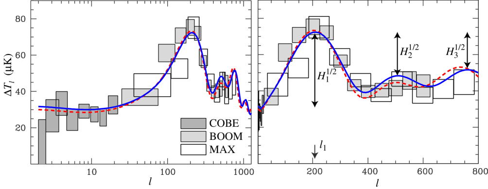
Figure 1.— Power spectrum data and models: (left panel) full range on a log scale; (right panel) first 3 peaks on a linear scale. The BOOMERanG (BOOM) and MAXIMA (MAX) points have been shifted by their 1$\sigma$ calibration errors, $10\%$ up and $4\%$ down respectively. Dashed lines represent a model that is a good fit to the CMB data alone: $\Omega_{m}=0.3$, $\Omega_{\Lambda}=0.7$, $h=0.9$, $\Omega_{b}h^{2}=0.03$, $n=1$ which gives $\ell_{1}=205$, $H_{1}=6.6$, $H_{2}=0.37$, $H_{3}=0.52$. Solid lines represent a model that is allowed by our joint constraints: $\Omega_{m}=0.35$, $\Omega_{\Lambda}=0.65$, $h=0.75$, $\Omega_{b}h^{2}=0.023$, $n=0.95$ which gives $\ell_{1}=209$, $H_{1}=5.8$, $H_{2}=0.45$, $H_{3}=0.5$. Note that the labelling of the $H$’s in the figure is schematic; these values are the power ratios as defined in the text.

Our main objective in this application is to clarify the constraints derived from the CMB observations using the likelihood analyses and understand how they might change as the data evolves. Then, with the aid of a few external constraints we map out the allowed region in the plane of the matter density ($\Omega_{m}$) versus the Hubble constant ($H_{0}$: we use $h$ to denote the Hubble constant $H_{0}=100h$ km s^-1Mpc^-1). The external constraints which we employ include (i) the rich cluster abundance at $z\approx 0$, (ii) the cluster baryon fraction, (iii) the baryon abundance from big bang nucleosynthesis (BBN), and (iv) the minimum age of the universe. We also discuss their consistency with other constraints, such as direct determinations of $H_{0}$, $\Omega_{m}$, and the luminosity distance to high redshift supernovae. All errors we quote in this paper are at 67% confidence, but we consider all constraints at a 95% confidence level.

In §2 we start with a statistical analysis of the CMB data. We introduce the four observables and discuss their cosmological implications. In §3, we place constraints on the $(\Omega_{m},h)$ plane and discuss consistency checks. In §4, we identify opportunities for future consistency checks and arenas for future confrontations with data. We conclude in §5. The appendix presents convenient formulae that quantify the cosmological parameter dependence of our four characteristic observables in adiabatic CDM models.

2. CMB Observables

2.1. Statistical Tests

With the present precision of the BOOMERanG and MAXIMA observations (see Fig. 1), it is appropriate to characterize the power spectrum with four numbers: the position of the first peak $\ell_{1}$, the height of the first peak relative to the power at $\ell=10$

$$H_{1}\equiv\left({\Delta T_{\ell_{1}}\over\Delta T_{10}}\right)^{2}\,,$$ (1)

the height of the second peak relative to the first

$$H_{2}\equiv\left({\Delta T_{\ell_{2}}\over\Delta T_{\ell_{1}}}\right)^{2}\,,$$ (2)

and the height of the third peak relative to the first

$$H_{3}\equiv\left({\Delta T_{\ell_{3}}\over\Delta T_{\ell_{1}}}\right)^{2}\,,$$ (3)

where $(\Delta T_{\ell})^{2}\equiv\ell(\ell+1)C_{\ell}/2\pi$ with $C_{\ell}$ the power spectrum of the multipole moments of the temperature field. Note that the locations of the second and third peaks are set by their harmonic relation to the first peak [see Appendix, eq. (A7)] and so $H_{2}$ and $H_{3}$ are well-defined even in the absence of clear detections of the secondary peaks.

One could imagine two different approaches towards measuring these four numbers. We could extract them using some form of parametrized fit such as a parabolic fit to the data (Knox & Page 2000; de Bernardis et al. 2000). Alternately, we could use template CDM models as calculated by CMBFAST (Seljak & Zaldarriaga 1996), and label them by the values of the four observables. We can measure $\chi^{2}$ for these CDM models and interpret them as constraints in the four observables. Both of these methods give similar results. We chose the second one because it is more stable to changes in the $\ell$ ranges taken to correspond to each peak and incorporates the correct shape of the power spectra for CDM-like models.

To determine the position of the first peak, we take the data that fall between $75<\ell<375$ and carry out a $\chi^{2}$ fitting using a flat model template ($\Omega_{\rm m}+\Omega_{\Lambda}=1$ here and below unless otherwise stated) with varying $h$ and $\Omega_{m}$ at the fixed baryon density $\Omega_{b}h^{2}=0.02$ and tilt parameter $n=1$. We include calibration errors, 10% for BOOMERanG and 4% for MAXIMA. Figure 2 shows $\Delta\chi^{2}$ as a function of $\ell_{1}$ for the BOOMERanG data alone and for the combination of BOOMERanG and MAXIMA. The figure implies

$$\ell_{1} = 200\pm 8\quad({\rm BOOM})\,,$$

$$\ell_{1} = 206\pm 6\quad({\rm BOOM+MAX})\,.$$ (4)

Other choices of $\Omega_{b}h^{2}$ and $n$ for the template parameters modify slightly the value of $\chi^{2}$ but not $\Delta\chi^{2}$ or the allowed region for $\ell_{1}$. It is noteworthy that adding in the MAXIMA data steepens $\Delta\chi^{2}$ on both sides of the minimum despite the preference for $\ell_{1}\sim 220$ in the MAXIMA data alone (Hanany et al. 2000). The fact that both data sets consistently indicate a sharp fall in power at $\ell>220$ increases the confidence level at which a high $\ell_{1}$ can be rejected.

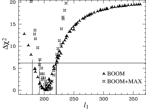
Figure 2.— Constraints on the first peak position: $\Delta\chi^{2}(\ell_{1})$ for the data from $75<\ell<375$. We define the $1\sigma$ errors to be $1/2.5$ of the errors at $2.5\sigma$ ($\Delta\chi^{2}=6.2$, solid lines).

The $H_{1}$ statistic depends both on the acoustic physics that determines the first peak and other processes relevant at $\ell\sim 10$. The shape of the template is therefore more susceptible to model parameters. We choose to vary $n$ which changes $H_{1}$ and also allow variations in $\Omega_{\Lambda}$ so that the position of the first peak can be properly adjusted. The other parameters were chosen to be $\Omega_{b}h^{2}=0.03$ and $\Omega_{m}h^{2}=0.2$. Using the BOOMERanG and MAXIMA data for $75<\ell<375$ in conjunction with the COBE data, we find

$$H_{1}=7.6\pm 1.4\ .$$ (5)

Other template choices can modify the constraint slightly but the errors are dominated by the COBE $7\%$ cosmic variance errors (Bunn & White 1997) and MAXIMA $4\%$ calibration errors on the temperature fluctuations.

Figure 3.— Constraint on the height of the second peak relative to the first: $\Delta\chi^{2}(H_{2})$ for the data from $75<\ell<600$. $1\sigma$ errors are defined as in Fig. 2.

For $H_{2}$, we take the data for $75<\ell<600$ and consider templates from models with varying $\Omega_{b}h^{2}$, $n$ and $\Omega_{\Lambda}$, where the last parameter is included to ensure that the models reproduce the position of the first peak. In this case, $\chi^{2}$ as a function of $H_{2}$ minimized over $\Omega_{\Lambda}$ exhibits some scatter due to information that is not contained in the ratio of the peak heights (see Fig. 3). Nonetheless, the steep dependence of $\Delta\chi^{2}$ on $H_{2}$ indicates that this statistic is robustly constrained against the variation of the template. Taking the outer envelope of $\Delta\chi^{2}$, we obtain

$$H_{2} = 0.37\pm 0.04\quad({\rm BOOM})\,,$$

$$H_{2} = 0.38\pm 0.04\quad({\rm BOOM+MAX})\,.$$ (6)

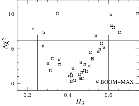
Figure 4.— Constraints on the height of the third peak relative to the first: $\Delta\chi^{2}(H_{3})$ for the data from $75<\ell<375$ and $600<\ell<800$. $1\sigma$ errors are defined as in Fig. 2.

$H_{3}$ is only weakly constrained by the two highest $\ell$ points ($600<\ell<800$) from MAXIMA in conjunction with the first peak data ($75<\ell<375$) from both experiments. We consider templates from models with varying $\Omega_{m}h^{2}$, $n$, $\Omega_{b}h^{2}$ and $\Omega_{\Lambda}$. The latter two parameters are included to ensure that the position of the first peak and the depth of the first trough can be modeled. Minimizing $\chi^{2}$ over these two parameters, we plot $\Delta\chi^{2}$ as a function of $H_{3}$ (see Fig. 4) to obtain the bound

$$H_{3}=0.43\pm 0.07\quad({\rm BOOM+MAX}).$$ (7)

Note that the constraints on $H_{3}$ employ a template-based extrapolation: points on the rise to the third peak are used to infer its height.

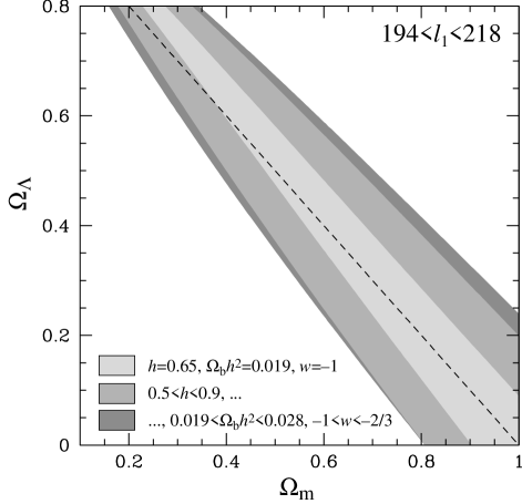
Figure 5.— Peak position constraint in the ($\Omega_{m}$, $\Omega_{\Lambda}$) plane with various priors. The prior assumptions weaken from the light shaded region to the dark shaded region and ’…’ means that the unlisted priors are unchanged from the neighboring region of stronger priors. The constrained region is strongly limited by the range in $h$ considered and to a lesser extent that in $\Omega_{b}h^{2}$ and the equation of state of $\Lambda$, $w$.

2.2. Cosmological Implications

The values for the four observables we obtained above can be used to derive and understand constraints on cosmological parameters from the experiments.

The position of the first peak as measured by $\ell_{1}$ is determined by the ratio of the comoving angular diameter distance to the last scattering epoch and the sound horizon at that epoch (Hu & Sugiyama 1995). Therefore it is a parameter that depends only on geometry and sound wave dynamics [see Appendix, eq. (A)] through $\Omega_{m}+\Omega_{\Lambda}$, $h$, $\Omega_{m}$, $w$, and $\Omega_{b}h^{2}$, in decreasing order of importance. The equation of state parameter $w=p_{\Lambda}/\rho_{\Lambda}$ with $p_{\Lambda}$ and $\rho_{\Lambda}$ the pressure and energy density of the vacuum $(w=-1)$ or negative-pressure energy; we use $\Lambda$ to refer to either option. The effect of tilt is small [see eq. (A8)]

$${\Delta\ell_{1}\over\ell_{1}}\approx 0.17(n-1)$$ (8)

and so we neglect it when considering models with $n\sim 1$.

Figure 5 displays the constraints in the $\Omega_{m}-\Omega_{\Lambda}$ plane. Notice that the confidence region is determined not by uncertainties in the measured value of $\ell_{1}$, but rather the prior assumptions about the acceptable range in $h$, $\Omega_{b}h^{2}$ and $w$ (Lange et al. 2000; Tegmark & Zaldarriaga 2000b). Given the broad consistency of the data with flat models ($\Omega_{\Lambda}+\Omega_{m}=1$) with $w=-1$, we will hereafter restrict ourselves to this class of models unless otherwise stated.

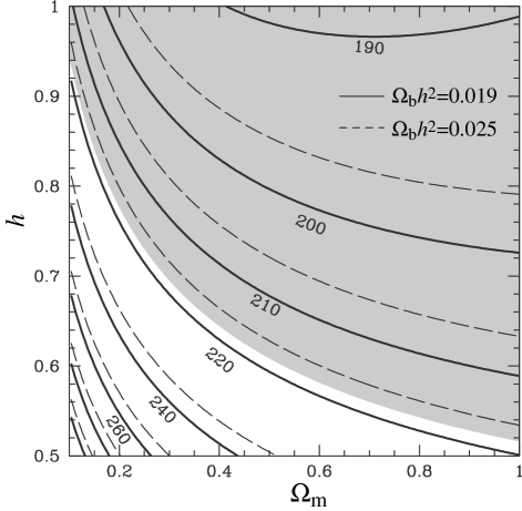
Figure 6.— Peak positions in the ($\Omega_{m}$,$h$) plane for $\Omega_{b}h^{2}=0.019$ and 0.025. Allowed region is indicated by hatching and assumes $\Omega_{b}h^{2}\geq 0.019$.

To better understand the dependence on the Hubble constant, we plot in Figure 6 contours of constant $\ell_{1}$ in the ($\Omega_{m}$,$h$) plane for $\Omega_{b}h^{2}=0.019$ and $\Omega_{b}h^{2}=0.025$. A higher baryon abundance decreases the sound horizon at last scattering and pushes up the contours in the direction of higher $\Omega_{m}$, $h$.

The 95% limit, $\ell_{1}<218$ from equation (4), excludes the lower left region shown in Figure 6. This limit derived from the curve for $\Omega_{b}h^{2}=0.019$ is robust in the sense that this baryon abundance represents the mimimum value allowed by the CMB, as we shall see later. This constraint is summarized approximately by $\Omega_{m}h^{3.8}>0.079$. The dependence differs from the familiar combination $\Omega_{m}h^{2}$ since in a flat universe part of the effect of lowering $\Omega_{m}$ is compensated for by the raising of $\Omega_{\Lambda}$. The lower limit on $\Omega_{m}h^{2}$ or equivalently on $\Omega_{m}$ found in Tegmark & Zaldarriaga (2000b) reflects the prior upper limit on $h$, e.g. for $h<0.8$, $\Omega_{m}h^{2}>0.12$ or $\Omega_{m}>0.18$.

The 95% confidence lower limit of the combined fit is $\ell_{1}>194$, but it does not give a robust limit in this plane in the absence of an upper limit on $\Omega_{b}h^{2}$. The lower limit is also less robust in the sense that it comes mainly from the MAXIMA result whereas both experiments agree on the upper limit in the sense that the addition of MAXIMA only serves to enhance the confidence at which we may regect larger values.

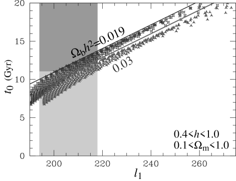
Figure 7.— Age-$\ell_{1}$ correlation. Points represent models in the $(\Omega_{m},h)$ plane. Lines represent the simple fit to the outer envelope given in eqn. (9) for the two choices of $\Omega_{b}h^{2}$. Light shaded region represents current constraints on $\ell_{1}$; dark shaded region is also consistent with $t_{0}>11$ Gyr.

For a flat geometry, the position of the first peak is strongly correlated with the age of the universe. The correlation is accidental since $\ell_{1}$ is the ratio of the conformal ages $\int dt/a$ at last scattering and the present that enters, not simply the physical age today. Nonetheless, Fig. 7 shows that the correlation is tight across the ($\Omega_{m}$, $h$) values of interest. The upper envelope corresponds to the lowest $\Omega_{m}$ $(=0.1)$ and implies

$$\left({t_{0}\over 1{\rm Gyr}}\right) \leq 19.7-0.155(250-\ell_{1})(0.68)^{1+w}$$ (9)

$$-\left(\Omega_{b}h^{2}\over 0.019\right)^{1.7}\,,$$

where we have included a weak scaling with $w$. The observations imply $t_{0}<13-14$ Gyr if $\Omega_{b}h^{2}\geq 0.019$. While this is a weak constraint given the current observational uncertainties, notice that the central value of the BOOMERanG results $\ell_{1}\approx 200$ would imply $t_{0}\approx 9-11$Gyrs.

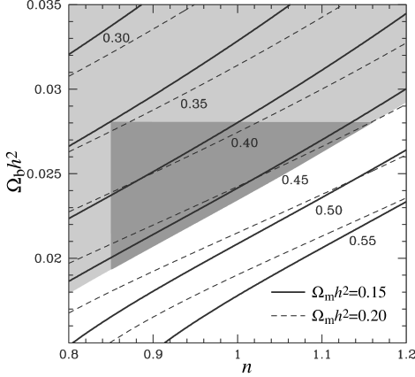
Figure 8.— Peak height ratio $H_{2}$ in the ($n$,$\Omega_{b}h^{2}$) plane for $\Omega_{m}h^{2}=0.15$ and 0.20. Allowed region is indicated by light shading and assumes $\Omega_{m}h^{2}\geq 0.15$. The constraint at $n\approx 1$ is nearly independent of this assumption. Dark shading indicates the region consistent with $H_{1}$ ($n>0.85$) and nucleosynthesis ($\Omega_{b}h^{2}<0.028$).

The $H_{2}$ statistic, the ratio of the heights of the second peak to the first, mainly depends on the tilt parameter and the baryon abundance. This combination is insensitive to reionization, the presence of tensor modes or any effects that are confined to the lowest multipoles. The remaining sensitivity is to $\Omega_{m}h^{2}$ and is modest in a flat universe due to the cancellation of two effects [see Appendix eq. (A19)]. Figure 8 shows contours of $H_{2}=$const. in the ($n,\Omega_{b}h^{2}$) plane for $\Omega_{m}h^{2}=0.15$ and $0.20$.

The result from the previous subsection, $H_{2}<0.46$ at a 95% confidence level is shown with shades, giving a constraint

$$\Omega_{b}h^{2}>0.029\left({\Omega_{m}h^{2}\over 0.15}\right)^{-0.58}(n-1)+0.024\,.$$ (10)

Note that the constraint at $n=1$ is approximately independent of $\Omega_{m}h^{2}$. This limit agrees well with the those from the detailed likelihood analysis of Tegmark & Zaldarriaga (2000b, c.f. their Fig. 4) under the same assumptions for $\Omega_{m}h^{2}$ and supports the claim that $H_{2}$ captures most of the information from the data on these parameters. An upper limit from $H_{2}>0.32$ also exists but is weaker than conservative constraints from nucleosynthesis as we discuss in the next section.

We can derive a limit on $n$ from the indicator $H_{1}$. The cosmological parameter dependence of $H_{1}$ is more complicated than the other two we discussed above. Fortunately, most complications tend to decrease $H_{1}$ by adding large angle anisotropies. The lower limit on $n$ from the lower limit on $H_{1}$ in the absence of e.g. reionization or tensor modes is therefore conservative. The upper limit on $n$ is very weak unless one excludes the possibility of tensor modes as a prior assumption (c.f. Balbi et al. ). We search for the minimum $n$ that gives $H_{1}$ larger than the 2$\sigma$ lower limit $H_{1}>4.8$ along the parameter space that maximizes $H_{2}$. This gives a conservative lower bound of $n>0.85$. This bound is to good approximation independent of $\Omega_{m}h^{2}$ for $\Omega_{m}h^{2}\gtrsim 0.15$. Below this value, the bound tightens marginally due to the integrated Sachs-Wolfe (ISW) effect on COBE scales, but in such a way so as to maintain the bound $\Omega_{b}h^{2}>0.019$ when combined with the constraint from $H_{2}$, the inequality (10). The analysis of Tegmark & Zaldarriaga (2000b) yields $n>0.87$ in the same parameter and data space indicating that not much information is lost in our much cruder parameterization.

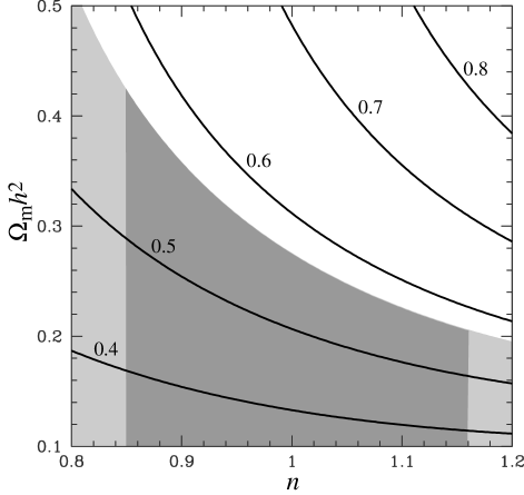
Figure 9.— Peak height ratio $H_{3}$ in the ($n$,$\Omega_{m}h^{2}$) plane for $H_{2}=0.38$. Allowed region is indicated by light shading. Darker shading indicates the allowed region with additional constraints from $H_{1}$ $(n>0.85)$ and nucleosynthesis $(\Omega_{b}h^{2}<0.028$, which gives $n<1.16$).

The $H_{3}$ statistic depends more strongly on $\Omega_{m}h^{2}$ and $n$ since the baryons affect the height of the third and first peak similarly. In Fig. 9, we show the constraint in the ($n$,$\Omega_{m}h^{2}$) plane with the baryon density fixed by requiring $H_{2}=0.38$. When combined with the constraint on the tilt $n>0.85$, we obtain $\Omega_{m}h^{2}<0.42$.

In Fig. 1 (dashed lines), we compare a model designed to have acceptable values for $\ell_{1}$, $H_{1}$, $H_{2}$ and $H_{3}$ with the power spectrum data from COBE, BOOMERanG and MAXIMA. This gives $\chi^{2}=27.2$ for 30 data points and compares well with the best fit model of Tegmark & Zaldarriaga (2000b) with their “inflation prior” where $\chi^{2}=26.7$. We summarize the constraints from the CMB as: $\Omega_{m}h^{3.8}$ $>0.079$ (or $t_{0}<14$ Gyr); $n>0.85$; $\Omega_{b}h^{2}>0.019$; $\Omega_{m}h^{2}<0.42$.

3. External Constraints

In this section, we combine the constraints from the CMB with those from four other observations: the light element abundances as interpreted by BBN theory, the present-day cluster abundance, the cluster baryon fraction and age of the universe. We then translate these constraints onto the ($\Omega_{m}$,$h$) plane and discuss consistency checks.

3.1. Nucleosynthesis

The first external constraint we consider is that on baryon abundance from primordial nucleosynthesis (see Copi et al. 1995; Olive et al. 1999; Tytler et al. 2000 for recent reviews). Olive et al.  (1999) give a high baryon density option of $0.015\leq\Omega_{b}h^{2}\leq 0.023$, and a low baryon density option $0.004\leq\Omega_{b}h^{2}\leq 0.010$ as a $2\sigma$ range. A low baryon density is indicated by the traditional low value of helium abundance ($Y_{p}=0.234\pm 0.003$) (Olive et al. 1999), and agrees with a literal interpretation of the lithium abundance. There are also two Lyman limit systems which taken at face value point to high deuterium abundance (Songaila et al 1994; Carswell et al. 1994; Burles et al. 1999a; Tytler et al. 1999) and implies a low baryon density.

Our lower limit on $\Omega_{b}h^{2}>0.019$ from $H_{2}$ and $H_{1}$ is strongly inconsistent with the low baryon abundance option. In fact our limit is only marginally consistent with even the high baryon option if we take the latest determination of the deuterium abundance at face value and treat the individual errors on the systems as statistical: D/H$=(3.4\pm 0.25)\times 10^{-5}$ from 3 Lyman limit systems (Kirkman et al. 2000) which implies $\Omega_{b}h^{2}=0.019\pm 0.0012$ (Tytler et al. 2000; Burles et al. 1999b). In this paper, we provisionally accept the 2$\sigma$ limit of Olive et al. (1999). The issue, however, is clearly a matter of systematic errors, and we discuss in what follows where they could appear, trying to find a conservative upper limit.

Since it is possible that the measured D/H abundance is high due to contamination by $H$, we consider the firm lower limit on the D/H abundance from interstellar clouds. The earlier UV data (McCullough 1992) show a variation of D/H from 1.2 to $2.5\times 10^{-5}$. This variation is confirmed by modern high resolution spectrographs. The clouds studied are still few in number and range from D/H=(1.5$\pm 0.1)\times 10^{-5}$ (Linsky 1998; Linsky et al. 1995) to $0.7\times 10^{-5}$ (Jenkins et al. 1999). This variation is reasonable since the clouds are contaminated by heavy elements, indicating significant astration effects. Therefore, we take the upper value as the observational D/H abundance, and take the minimum astration effect (factor 1.5) from model calculations (see Tosi 1996; Olive et al. 1999, modified for a 10 Gyr disk age) to infer the lower limit on the primordial deuterium abundance. We take $2\times 10^{-5}$ as a conservative lower limit on D/H. This value agrees with the pre-solar system deuterium abundance inferred from ³He (Gloeckler & Geiss 1998). This D/H corresponds to $\Omega_{b}h^{2}=0.028$ and $Y_{p}=0.250-0.252$.

The helium abundance $Y_{p}$ directly depends on the theoretical calculation of the helium recombination line, and the discrepancy between the estimate ($Y_{p}=0.244\pm 0.002$, Izotov & Thuan 1998) and the traditional estimates ($Y_{p}=0.234\pm 0.003$) largely arises from the two different calculations, Smits (1996) and Blocklehurst (1972). The helium abundances derived from three recombination lines He I $\lambda$4471, $\lambda$5876 and $\lambda$6678 for a given HII region differ fractionally by a few percent. Also, the effect of underlying stellar absorption by hot stars is unclear: Izotov & Thuan (1998) use the departure of the He I $\lambda 6678/\lambda 5876$ strengths from the Smits calculation as an estimator, but a calculation is not actually available for the He line absorption effect. While these variations are usually included as random errors in the nucleosynthesis literature, we suspect that the error in the helium abundance is dominated by systematics and a further change by a few percent in excess of the quoted range is not excluded.

The interpretation of the Li abundance rests on a simplistic model of stars. It seems that our understanding of the ⁷Li abundance evolution is still far from complete: for instance we do not understand the temperature gradient of the Li/H ratio in halo dwarfs, which shows a trend opposite to what is expected with ⁷Li destruction due to diffusion. Hence we do not view the primordial ⁷Li abundance determinations as rock-solid.

We therefore consider two cases $\Omega_{b}h^{2}<0.023$ as a widely accepted upper limit and $\Omega_{b}h^{2}<0.028$ as a very conservative upper limit based on interstellar deuterium. When combined with the limit of eq. (10), the latter constraint becomes $n<1.16$ for $\Omega_{m}h^{2}<0.2$ (as appropriate for setting a lower bound on $\Omega_{m}$ in the next section, see also Fig. 9); if we instead take $\Omega_{b}h^{2}<0.023$ (Olive et al. 1999), the limit becomes $n<0.98$. In conjunction with the constraint from $H_{1}$, the allowed range for the tilt becomes

$$0.85<n<1.16\,.$$ (11)

3.2. Cluster Abundance

The next external constraint we consider is the abundance of clusters of galaxies, which constrains the matter power spectrum at intermediate scales. We adopt the empirical fit of Eke et al. (1996) for a flat universe $\sigma_{8}=(0.52\pm 0.08)\Omega_{m}^{-0.52+0.13\Omega_{m}}$. The value of $\sigma_{8}$ is well converged within 1 $\sigma$ among different authors (Viana & Liddle 1999; Pen 1998). This is because the cluster abundance depends strongly on $\sigma_{8}$ due to its appearance in the exponential of a Gaussian in the Press-Shechter formalism.

We take the amplitude at COBE scales with a 14 % normalization uncertainty (95 % confidence) together with the 95 % confidence range coming from the cluster abundance to obtain an allowed region that is a function of $\Omega_{m}$, $h$ and $n$ and can be roughly described by

$$0.27<\Omega_{m}^{0.76}hn<0.35\,,$$ (12)

assuming no tensor contribution to COBE and $\Omega_{b}h^{2}=0.028$. These assumptions lead to the most conservative constraints on the ($\Omega_{m}$,$h$) plane. The lower limit comes from undershooting $\sigma_{8}$ which is only exacerbated with the inclusion of tensors. It also depends on the upper limit on $n$, which is maximized at the highest acceptable baryon density $\Omega_{b}h^{2}=0.028$. The upper limit comes from overshooting $\sigma_{8}$ and depends on the lower limit on $n$, which only tightens with the inclusion of tensors and lowering of the baryon density.

3.3. Baryon Fraction

The third external constraint we consider is the baryon fraction in rich clusters, derived from X-ray observations. The observed baryon fraction shows a slight increase outwards, and the true baryon fraction inferred for the entire cluster depends on the extrapolation. The estimates range from $(0.052\pm 0.0025)h^{-3/2}$ (White & Fabian 1995; lowest estimate) to $(0.076\pm 0.008)h^{-3/2}$ (Arnaud & Evrard 1999; highest estimate) for rich clusters. We take the 2$\sigma$ limits to correspond to these two extreme values. We remark that very similar constraints are derived from the Sunyaev Zeldovich effect for clusters as long as $h=0.5-1.0$: Myers et al. (1997) derive $(0.061\pm 0.011)h^{-1}$, and Grego et al. (2000) give $(0.074\pm 0.009)h^{-1}$. Adding baryons locked into stars to that in gas inferred by $X$-ray observations, and assuming the cluster baryon fraction represents the global value (White et al. 1993), we have $f_{b}\equiv\Omega_{b}/\Omega_{m}$ constrained as

$$0.052h^{-3/2}+0.006h^{-1}<f_{b}<0.076h^{-3/2}+0.015h^{-1}$$ (13)

This relation is used to convert the constraints on $\Omega_{b}h^{2}$ into the $\Omega_{m}$ vs $h$ plane.

3.4. Age

We take the lower limit on the age of the universe to be $t_{0}>11$Gyr based on stellar evolution. While this is not based on statistical analysis, no authors have ever claimed a cosmic age less than this value (Gratton et al. 1997; Reid 1997; Chaboyer et al. 1998).

3.5. Allowed Region

We display all our constraints in the ($\Omega_{m}$,$h$) plane in Fig. 10.

Combining the range $0.019\leq\Omega_{b}h^{2}\leq 0.028$ from BBN and the CMB, together with the constraint on $\Omega_{b}/\Omega_{m}$ from the baryon fraction (13) leads to the range

$${0.019\over 0.076h^{1/2}+0.015h}<\Omega_{m}<{0.028\over 0.052h^{1/2}+0.006h}\,,$$ (14)

which is plotted as the solid contours labeled $f_{b}$ in Fig. 10. We also plot the more conservative limits derived from taking the $2\sigma$ extremes of the extreme baryond fraction measures ($0.076\rightarrow 0.092$ and $0.052\rightarrow 0.047$) as dashed lines.

We convert the cluster abundance constraint using the range in tilts acceptable from the CMB constraints and the limit $\Omega_{b}h^{2}<0.028$ from BBN ($0.85<n<1.16$) and find

$$0.15<\Omega_{m}h^{1.3}<0.32\,.$$ (15)

This range is displayed by the contours labelled “$\sigma_{8}$”. Finally the constraints $t_{0}>11$Gyr and $\ell_{1}<218$ are labelled as “$t_{0}$” and “$\ell_{1}$” respectively.

The shading indicates the parameter space within which a model consistent with the CMB and external constraints may be constructed. Dark shading indicates the region that is also consistent with the stronger nucleosynthesis bound of $\Omega_{b}h^{2}<0.023$. This does not mean that all models in this region are consistent with the CMB data. To construct a viable model for a given ($\Omega_{m}$,$h$) in this region, one picks a tilt $n$ between $0.85-1.16$ consistent with the cluster abundance constraint (12) and then a baryon density consistent with $H_{2}$ (10) and $\Omega_{b}h^{2}<0.028$ (or $0.023$). In Fig. 1 (solid lines), we verify that the power spectrum prediction of a model so constructed is a good fit to the data. Here $\chi^{2}=28.5$ for the 30 data points to be compared with $\chi^{2}=27.2$ for the model optimized for the CMB alone.

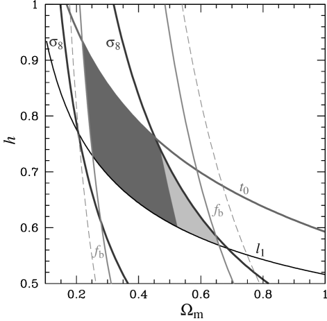
Figure 10.— Summary of constraints. The shaded region is allowed by all constraints considered in this paper. The dark shaded region contains models that are also consistent with $\Omega_{b}h^{2}<0.023$ (see text).

3.6. Consistency Checks

There are a variety of other cosmological measurements that provide alternate paths to constraints in the ($\Omega_{m}$,$h$) plane. We do not use these measurements as constraints since a proper error analysis requires a detailed consideration of systematic errors that is beyond the scope of this paper. We instead use them as consistency checks on the adiabatic CDM framework.

Hubble constant. A combined analysis of secondary distance indicators gives $h=0.71\pm 0.04$ for an assumed LMC distance of 50 kpc (Mould et al. 2000). Allowing for a generous uncertainty in the distance to the LMC (see Fukugita 2000 for a review) these values may be multiplied by $0.95-1.15$ and this should be compared with our constraint of $0.6<h<0.9$.

Cosmic acceleration. The luminosity distance to distant supernovae requires $\Omega_{m}<0.48$ for flat $\Lambda$ models if the systematic errors are no worse than they are claimed (Riess et al 1998; Perlmutter et al. 1999). This limit should be compared with our constraint of $\Omega_{m}<0.6$.

Mass-to-Light Ratio. The $\Omega_{m}$ constraint we derived using the range $0.019<\Omega_{b}h^{2}<0.023$ (see Fig. 10, dark shaded region) and the cluster baryon fraction corresponds to $M/L_{B}=(350-600)h$, which is roughly consistent with $M/L_{B}$ for rich clusters (e.g. Carlberg et al. 1997). A yet larger $\Omega_{m}$ ($\Omega_{m}>0.45$) would imply the presence of a substantial amount of matter outside clusters and galaxies, whereas we have some evidence indicating the contrary (Kaiser et al. 1998).

Power Spectrum. The shape parameter of the transfer function is $\Gamma\approx\Omega_{m}h\exp[-\Omega_{b}(1-1/\Omega_{m})]\approx 0.22-0.33$ for our allowed region (Sugiyama 1995). This is close to the value that fits the galaxy power spectrum; $\Gamma=0.2-0.25$ (Efstathiou et al. 1990; Peacock & Dodds 1994). On smaller scales, the Ly$\alpha$ forest places constraints on the amplitude and slope of the power spectrum near $k\sim 1$ $h$ Mpc^-1 at $z\sim 3$ (Croft et al. 1999; McDonald et al 1999). McDonald et al (1999) map these constraints onto cosmological parameters within $\Lambda$CDM as $n=0.93\pm 0.10$ and $\sigma_{8}=0.68+1.16(0.95-n)\pm 0.04$.

Cluster Abundance Evolution. The matter density $\Omega_{m}$ can be inferred from evolution of the rich cluster abundance (Oukbir & Blanchard 1992), but the result depends sensitively on the estimates of the cluster masses at high redshift. Bahcall & Fan (1998) argue for a low density universe $\Omega_{m}=0.2{+0.3\atop-0.1}$; Blanchard & Bartlett (1998) and Reichart et al. (1999) favor a high density $\Omega\approx 1$, while Eke et al. (1998) obtain a modestly low density universe $\Omega_{m}=0.36\pm 0.25$.

Peculiar Velocities. The results from peculiar velocity flow studies are controversial: they vary from $\Omega_{m}=0.15$ to 1 depending on scale, method of analysis and the biasing factor (see e.g. Dekel 1999 for a recent review).

Local Baryons. The CMB experiments require a high baryon abundance. The lower limit (together with a modest red-tilt of the spectrum) is just barely consistent with the high baryon abundance option from nucleosynthesis. The required baryon abundance is still below the maximum estimate of the baryon budget in the local universe $0.029h^{-1}$ (Fukugita et al. 1998), but this requires 3/4 of the baryons to reside near groups of galaxies as warm and cool gas.

4. Future Directions and Implicit Assumptions

A useful aspect of our approach is that one can ask how the allowed parameter space might evolve as the data evolves. More specifically, what aspect of the data can make the allowed region qualitatively change or vanish altogether? If the data are taken at face value, what theoretical assumptions might be modified should that come to pass?

An increase in the precision with which the acoustic scale is measured may lead to a new age crisis. It is noteworthy that the secondary peaks will eventually provide a substantially more precise determination of the scale due to sample variance limitations per patch of sky, the multiplicity of peaks, and the effects of driving forces and tilt on the first peak [see Appendix eq. (A7)]. Indeed, consistency between the determinations of this scale from the various peaks will provide a strong consistency check on the underlying framework. If the measurements were to determine an equivalent $\ell_{1}\leq 200$, then $t_{0}<10-11$Gyrs in a flat $\Lambda$ cosmology with $\Omega_{b}h^{2}=0.019$; taking $\Omega_{b}h^{2}=0.03$ decreases the age by 1 Gyr and exacerbates the problem. Such a crisis, should it occur, can only be mildly ameliorated by replacing the cosmological constant with a dynamical “quintessence” field. Because increasing the equation of state $w$ from $-1$ reduces both $\ell_{1}$ and the age, only a relatively extreme choice of $w\gtrsim-1/3$ can help substantially [see eqn. (9)]. This option would also imply that the universe is not accelerating and is in conflict with evidence from distant supernovae. However, other solutions may be even more unpalatable: a small positive curvature and a cosmological constant or a delay in recombination.

As constraints on the tilt improve by extending the dynamic range of the CMB observations and those on $H_{2}$ by resolving the second peak, one might be faced with a baryon crisis. Already $\Omega_{b}h^{2}=0.019$ is only barely allowed at the 95% CL. Modifications of big-bang nucleosynthesis that allow a higher baryon density for the same deuterium abundance are difficult to arrange: current directions of study include inhomogeneous nucleosynthesis (e.g. Kainulainen et al. 1999) and lepton asymmetry (e.g. Lesgourgues & Peloso 2000; Esposito et al. 2000). On the CMB side, there are two general alternatives. The first possibility is that there is a smooth component that boosts the relative height of the first peak (Bouchet et al. 2000). That possibility can be constrained in the same way as tilt: by extending the dynamic range, one can distinguish between smooth and modulated effects. The direct observable in the modulation is the ratio of energy densities in non-relativistic matter that is coupled to the CMB versus the CMB itself [$R_{*}$, see eqn. (A4)], times the gravitational potential, all evaluated at last scattering. The second possibility is that one of the links in the chain of reasoning from the observables to the baryon and matter densities today is broken in some way.

It is noteworthy that there is no aspect of the CMB data today that strongly indicates missing energy in the form of a cosmological constant or quintessence. An Einstein-de Sitter universe with a high baryon density is still viable unless external constraints are introduced. Under the assumption of a flat $\Lambda$ cosmology, tight constraints on $\Omega_{m}h^{3.8}$ from the peak locations and $\Omega_{m}h^{2}$ from the third and higher peak heights should allow $\Omega_{m}$ and $h$ to be separately measured. It will be important to check whether the CMB implications for $\Omega_{m}$ are consistent with external constraints.

Aside from acceleration measurements from distant supernovae, the missing energy conclusion finds its strongest support from the cluster abundance today through $\sigma_{8}$ and the cluster baryon fraction. Changes in the interpretation of these measurements would affect the viability of the Einstein-de Sitter option.

The interpretation of the cluster abundance is based on the assumption of Gaussian initial conditions and the ability to link the power spectrum today to that of the CMB through the usual transfer functions and growth rates. One possibility is that the primordial power spectrum has strong deviations from power-law behavior (e.g. Adams et al. 1997). Just like tilt, this possibility can be constrained through the higher peaks.

A more subtle modification would arise if the neutrinos had a mass in the eV range. Massive neutrinos have little effect on the CMB itself (Dodelson et al. 1996; Ma & Bertschinger 1995) but strongly suppress large scale structure through growth rates (Jing et al. 1993; Klypin et al. 1993). A total mass (summed over neutrino species) of $\sum{m_{\nu_{i}}}=1$eV would be sufficient to allow an Einstein-de Sitter universe in the cluster abundance. One still violates the cluster baryon fraction constraint. In fact, even for lower $\Omega_{m}$ one can only find models consistent with both the cluster abundance and baryon fraction if $\sum{m_{\nu_{i}}}<4$eV. These constraints could be weakened if some unknown form of support causes an underestimate of the dark mass in clusters through the assumption of hydrostatic equilibrium. They could also be evaded if modifications in nucleosynthesis weaken the upper limit on the baryons.

5. Conclusions

We find that the current status of CMB power spectrum measurements and their implications for cosmological parameters can be adequately summarized with four numbers: the location of the first peak $\ell_{1}=206\pm 6$ and the relative heights of the first three peaks $H_{1}=7.6\pm 1.4$, $H_{2}=0.38\pm 0.04$ and $H_{3}=0.43\pm 0.07$. When translated into cosmological parameters, they imply $\Omega_{m}h^{3.8}>0.079$ (or $t_{0}<13-14$ Gyr), $n>0.85$, $\Omega_{b}h^{2}>0.019$, $\Omega_{m}h^{2}<0.42$ for flat $\Lambda$CDM models. Other constraints mainly reflect the implicit (with priors) or explicit use of information from other aspects of cosmology. For example, our consideration of nucleosynthesis, the cluster abundance, the cluster baryon fraction, and the age of the universe leads to an allowed region where $0.6<h<0.9$, $0.25<\Omega_{m}<0.45$, $0.85<n<0.98$, $0.019<\Omega_{b}h^{2}<0.023$. The region is narrow, but there clearly are adiabatic CDM models viable at the $95\%$ CL as exemplified in Fig. 1. The region widens and the quality of the fit improves if one allows somewhat higher baryons $\Omega_{b}h^{2}<0.028$ as discussed in this paper. With this extension the tilt can be larger than unity $n<1.16$ and $\Omega_{m}$ as high as 0.6. We note that in both cases our limits reflect conservative assumptions about tensors and reionization, specifically that they are negligible effects in the CMB.

The constraints on these and other CMB observables are expected to rapidly improve as new data are taken and analyzed. We have identified sets of observables that should provide sharp consistency tests for the assumptions that underly their translation into cosmological parameters in the adiabatic CDM framework.

With the arrival of precision data sets, the enterprise of measuring cosmological parameters from the CMB has entered a new era. Whether the tension between the observations that is confining the standard parameters to an ever tightening region is indicating convergence to a final solution or hinting at discord that will challenge our underlying assumptions remains to be seen.

Appendix A Scaling Relations

The phenomenology of the peaks can be understood through three fundamental scales which vary with cosmological parameters: the acoustic scale $\ell_{A}$, the equality scale $\ell_{\rm eq}$ and the damping scale $\ell_{D}$.

We begin by employing an idealized picture of the photon-baryon fluid before recombination that neglects dissipation and time variation of both the sound speed $c_{s}$ and the gravitational driving forces. Simple acoustic physics then tells us that the effective temperature perturbation in the wavemode $k$ oscillates as (Hu & Sugiyama 1995)

$$\Delta T(\eta_{*},k)=[\Delta T(0,k)+R_{*}\Psi]\cos(ks_{*})-R_{*}\Psi\,.$$ (A1)

where the sound horizon at the last scattering surface $s\equiv\int c_{s}d\eta=\int c_{s}dt/a$ with $c_{s}^{2}=1/3(1+R)$ and $R=3\rho_{b}/4\rho_{\gamma}$. $\Psi$ is the gravitational potential. The asterisk denotes evaluation at last scattering. Baryons modulate the amplitude of the oscillation by shifting the zero point by $R_{*}\Psi$. The result is that the modes that reach maximal compression inside potential wells at last scattering are enhanced over those that reach maximal rarefaction. Note that this amplitude modulation is not equivalent to saying that the hot spots are enhanced over cold spots as the same reasoning applies to potential “hills”.

The oscillator equation (A1) predicts peaks in the angular power spectrum at $\ell_{m}=m\ell_{A}$ where $\ell_{A}$ is related to $s_{*}$ through its projection on the sky today via the comoving angular diameter distance (Hu & Sugiyama 1995)

$$D \approx 2{[1+\ln(1-\Omega_{\Lambda})^{0.085}]^{1+1.14(1+w)}\over\sqrt{\Omega_{m}H_{0}^{2}\Omega_{\rm t}^{(1-\Omega_{\Lambda})^{-0.76}}}}$$ (A2)

$$\equiv {2d\over\sqrt{\Omega_{m}H_{0}^{2}}}\,,$$

where $\Omega_{\Lambda}$ refers to the density in dark energy with a fixed equation of state $w=p_{\Lambda}/\rho_{\Lambda}$ ($w=-1$ for a true cosmological constant) and the total density is $\Omega_{\rm t}=\Omega_{m}+\Omega_{\Lambda}$. For convenience, we have defined the dimensionless angular diameter distance $d$ which scales out the effect of the expansion rate during matter domination; hence it is equal to unity for an Einstein-de Sitter cosmology. More specifically, $\ell_{A}\equiv\pi D/s_{*}$ or

$$\ell_{A} \approx {172d}\left({z_{*}\over 10^{3}}\right)^{1/2}$$

$$\times\left({1\over\sqrt{R_{*}}}\ln{\sqrt{1+R_{*}}+\sqrt{R_{*}+r_{*}R_{*}}\over 1+\sqrt{r_{*}R_{*}}}\right)^{-1}\,,$$

where the radiation-to-matter and baryon-to-photon ratios at last scattering are

$$r_{*} \equiv \rho_{r}(z_{*})/\rho_{m}(z_{*})=0.042\omega_{m}^{-1}(z_{*}/10^{3})\,,$$

$$R_{*} \equiv 3\rho_{b}(z_{*})/4\rho_{\gamma}(z_{*})=30\omega_{b}(z_{*}/10^{3})^{-1}\,$$ (A4)

with a redshift of last scattering given by

$$z_{*} \approx 1008(1+0.00124\omega_{b}^{-0.74})(1+c_{1}\omega_{m}^{c_{2}})\,,$$

$$c_{1} = 0.0783\omega_{b}^{-0.24}(1+39.5\omega_{b}^{0.76})^{-1}\,,$$

$$c_{2} = 0.56(1+21.1\omega_{b}^{1.8})^{-1}\,.$$ (A5)

Here we use the shorthand convention $\omega_{b}=\Omega_{b}h^{2}$ and $\omega_{m}=\Omega_{m}h^{2}$. Baryon drag works to enhance $m=$odd over $m=$even peaks in the power.

These simple relations are modified by driving and dissipative effects. The driving effect comes from the decay of the gravitational potential in the radiation dominated epoch which enhances the oscillations and leads to an increase in power of approximately a factor of 20 for $\ell>\ell_{\rm eq}$ (Hu & Sugiyama 1995) where

$$\ell_{\rm eq}\equiv(2\Omega_{m}H_{0}^{2}z_{\rm eq})^{1/2}D\approx{438d}\omega_{m}^{1/2}\,.$$ (A6)

It also introduces a phase shift to the oscillations such that the $m$th peak of a scale invariant ($n=1$ model) is at

$$\ell_{m} = \ell_{A}(m-\phi)$$

$$\phi \approx 0.267\left({r_{*}\over 0.3}\right)^{0.1}\,.$$ (A7)

Tilt also mildly affects the location of the peaks especially the first which is broadened by radiation effects; around $n=1$ (and $\Omega_{m}h^{2}=0.15$), the change is approximately

$${\Delta\ell_{1}\over\ell_{1}} \approx 0.17(n-1)\,,$$

$${\Delta\ell_{2}\over\ell_{2}} \approx 0.033(n-1)\,,$$

$${\Delta\ell_{3}\over\ell_{3}} \approx 0.012(n-1).$$ (A8)

The matter dependence is weak: for $\Omega_{m}h^{2}=0.25$ the coefficient $0.17$ is reduced to $0.15$ for $\ell_{1}$.

The other effect of radiation driving is to reduce the baryon drag effect by reducing the depth of the potential wells at $z_{*}$. The baryon drag effect is fractionally of order $R_{*}\Psi(\eta_{*})/\Psi(\eta_{\rm initial})\approx R_{*}T(k)$ where $T(k)$ is the matter transfer function and $k$ is the comoving wavenumber in Mpc^-1. The transfer function quantifies the decay of the potential in the radiation dominated epoch (see e.g. Eisenstein & Hu 1999 for a fit). The break in the transfer function is also given by the horizon scale at matter-radiation equality so that it appears on the sky at $\ell_{\rm eq}$. Shifting the equality scale to raise $\ell_{\rm eq}$ by raising the matter content decreases the overall amplitude of the oscillations but increases the odd-even modulation leading to somewhat counterbalancing effects on the peak heights.

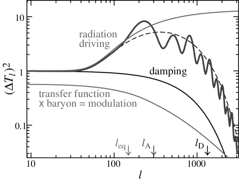
Figure 11.— A model power spectrum based on the fundamental scales $\ell_{\rm A}$, $\ell_{\rm eq}$, $\ell_{\rm D}$ and the baryon-photon ratio $R_{*}$ which modulates the amplitude of the oscillations as $R_{*}T(\ell/D)$ where $T(k)$ is the transfer function.

Finally, the acoustic oscillations are dissipated on small scales. The quantitative understanding of the effect requires numerical calculation but its main features can be understood through qualitative arguments. Since the oscillations dissipate by the random walk of the photons in the baryons, the characteristic scale for the exponential damping of the amplitude is the geometric mean between the mean free path $\lambda_{C}=(x_{e}n_{e}\sigma_{T}a)^{-1}$ and the horizon scale

$$\eta_{*}=2(\Omega_{m}H_{0}^{2})^{-1/2}z_{*}^{1/2}[\sqrt{1+r_{*}}-\sqrt{r_{*}}]\,.$$ (A9)

under the Saha approximation $x_{e}\propto\omega_{b}^{-1/2}$ so that $k_{D}\sim(\eta_{*}\lambda_{C})^{-1/2}\propto z_{*}^{5/4}\omega_{b}^{1/4}\omega_{m}^{1/4}$. Numerically, the scaling is slightly modified to (refitting values from Hu & White 1997)

$$\ell_{D}\equiv k_{D}D\approx{2240d\over[(1+r_{*})^{1/2}-r_{*}^{1/2}]^{1/2}}\left({z_{*}\over 1000}\right)^{5/4}\omega_{b}^{0.24}\omega_{m}^{-0.11}\,.$$ (A10)

Compared with the acoustic scale $\ell_{A}$, it has a much stronger dependence on $\omega_{b}$ and the redshift of recombination $z_{*}$. We show a model spectrum obtained this way for a $\Lambda$CDM cosmology with $\Omega_{m}=0.35$, $\Omega_{\rm t}=1$, $h=0.65$, $\omega_{b}=0.02$, and $w=-1$ in Fig. 11. For this cosmology, the three fundamental scales are $\ell_{\rm eq}=149$ ($\ell_{1}=221$), $\ell_{A}=301$, and $\ell_{D}=1332$. The dependence of the morphology of the acoustic peaks on cosmological parameters is controlled by these three scales. Around the fiducial $\Lambda$CDM model with the parameters given above

$${\Delta\ell_{A}\over\ell_{A}} \approx -0.11\Delta w-0.24{\Delta\omega_{m}\over\omega_{m}}+0.07{\Delta\omega_{b}\over\omega_{b}}$$ (A15)

$$\quad-0.17{\Delta\Omega_{\Lambda}\over\Omega_{\Lambda}}-1.1{\Delta\Omega_{\rm t}\over\Omega_{\rm t}}$$

$$\approx -0.11\Delta w-0.48{\Delta h\over h}+0.07{\Delta\omega_{b}\over\omega_{b}}-0.15{\Delta\Omega_{m}\over\Omega_{m}}$$

$$\quad-1.4{\Delta\Omega_{\rm t}\over\Omega_{\rm t}}\,,$$

where the leading order dependence is on $\Omega_{\rm t}$ and $h$

$${\Delta\ell_{\rm eq}\over\ell_{\rm eq}} \approx -0.11\Delta w+0.5{\Delta\omega_{m}\over\omega_{m}}-0.17{\Delta\Omega_{\Lambda}\over\Omega_{\Lambda}}-1.1{\Delta\Omega_{\rm t}\over\Omega_{\rm t}}$$ (A16)

$$\approx -0.11\Delta w+{\Delta h\over h}+0.59{\Delta\Omega_{m}\over\Omega_{m}}-1.4{\Delta\Omega_{\rm t}\over\Omega_{\rm t}}\,,$$

which depends more strongly on $\Omega_{m}$, and

$${\Delta\ell_{D}\over\ell_{D}} \approx -0.11\Delta w-0.21{\Delta\omega_{m}\over\omega_{m}}+0.20{\Delta\omega_{b}\over\omega_{b}}$$ (A17)

$$\quad-0.17{\Delta\Omega_{\Lambda}\over\Omega_{\Lambda}}-1.1{\Delta\Omega_{\rm t}\over\Omega_{\rm t}}$$

$$\approx -0.11\Delta w-0.42{\Delta h\over h}+0.20{\Delta\omega_{b}\over\omega_{b}}$$

$$\quad-0.12{\Delta\Omega_{m}\over\Omega_{m}}-1.4{\Delta\Omega_{\rm t}\over\Omega_{\rm t}}\,.$$

which depends more strongly on the baryon abundance $\omega_{b}$. Note that the sensitivity to $\Omega_{\rm t}$ increases from the often quoted $-0.5\Delta\Omega_{\rm t}/\Omega_{\rm t}$ as $\Omega_{\Lambda}$ increases (Weinberg 2000; M. Turner, private communication).

Ideally one would like to extract these three numbers and the baryon-photon ratio $R_{*}$ directly from the data. The acoustic scale is readily extracted via the position of the first and/or other higher peaks. The other quantities however are less directly related to the observables. We instead choose to translate the parameter dependence into the space of the observations: in particular the height of the first three peaks.

The height of the first peak

$$H_{1}\equiv\left({\Delta T_{\ell_{1}}\over\Delta T_{10}}\right)^{2}\,.$$ (A18)

may be raised by increasing the radiation driving force (lowering $\ell_{\rm eq}$ or $\omega_{m}$) or the baryon drag (raising $\omega_{b}$). However it may also be lowered by filling in the anisotropies at $\ell\approx 10$ through the ISW effect (raising $\Omega_{\Lambda}$ or $w$, or lowering $\Omega_{\rm t}$), reionization (raising the optical depth $\tau$), or inclusion of tensors. Each of the latter effects leaves the morphology of the peaks essentially unchanged. Because $H_{1}$ depends on many effects, there is no simple fitting formula that describes it. Around the $\Lambda$CDM model with $H_{1}=7.4$, it is crudely

$${\Delta H_{1}\over H_{1}} \sim -0.5{\Delta\omega_{m}\over\omega_{m}}+0.4{\Delta\omega_{b}\over 0.02}-0.5{\Delta\Omega_{\Lambda}}+0.7{\Delta\Omega_{\rm t}}$$

$$\quad 2.5{\Delta n}-1{\Delta\tau}-0.3{\Delta w}-0.76{\Delta r\over 1+0.76r}\,.$$

where the tensor contribution $r\equiv 1.4(\Delta T_{10}^{\rm(T)}/\Delta T_{10}^{\rm(S)})^{2}$. This scaling should only be used for qualitative purposes.

The height of the second peak relative to the first is written

$$H_{2}\equiv\left(\Delta T_{\ell_{2}}\over\Delta T_{\ell_{1}}\right)^{2}\approx{0.925\omega_{m}^{0.18}(2.4)^{n-1}\over[1+(\omega_{b}/0.0164)^{12\omega_{m}^{0.52}}]^{1/5}}\,,$$ (A19)

where $n$ is the scalar tilt and $\ell_{2}/\ell_{1}\approx 2.4$. This approximation breaks down at high $\omega_{b}$ and $\omega_{m}$ as the second peak disappears altogether. In the $\Lambda$CDM model with $n=1$, $H_{2}=0.51$ and parameter variations yield

$${\Delta H_{2}\over H_{2}}\approx 0.88\Delta n-0.64{\Delta\omega_{b}\over\omega_{b}}+0.14{\Delta\omega_{m}\over\omega_{m}}\,.$$ (A20)

The effect of tilt is obvious. Baryons lower $H_{2}$ by increasing the modulation that raises all odd peaks. The dependence on the matter comes from two competing effects which nearly cancel around the $\Lambda$CDM: increasing $\omega_{m}$ (lowering $\ell_{\rm eq}$) decreases the radiation driving and increases $H_{2}$ but also increases the depth of potential wells and hence the modulation that lowers $H_{2}$.

For the third peak, these effects add rather than cancel. When scaled to the height of the first peak, which is also increased by raising the baryon density, the $\Omega_{b}h^{2}$ dependence weakens leaving a strong dependence on the matter density

$$H_{3} \equiv \left(\Delta T_{\ell_{3}}\over\Delta T_{\ell_{1}}\right)^{2}$$ (A21)

$$\approx 2.17\left[1+\left({\omega_{b}\over 0.044}\right)^{2}\right]^{-1}\omega_{m}^{0.59}(3.6)^{n-1}$$

$$\quad\times\left[1+1.63\left(1-{\omega_{b}\over 0.071}\right)\omega_{m}\right]^{-1}$$

where $\ell_{3}/\ell_{1}\approx 3.6$. Around the fiducial $\Lambda$CDM model where $H_{3}=0.50$

$${\Delta H_{3}\over H_{3}}\approx 0.41\Delta n-0.31{\Delta\omega_{b}\over\omega_{b}}+0.53{\Delta\omega_{m}\over\omega_{m}}\,.$$ (A22)

We emphasize that the phenomenology in terms of $\ell_{A}$, $\ell_{\rm eq}$ and $\ell_{D}$ is relatively robust, predictive of morphology beyond the first three peaks and readily generalizable to models outside the adiabatic cold dark matter paradigm. The specific scalings of $H_{1}$, $H_{2}$ and $H_{3}$ with cosmological parameters are only valid within the family of adiabatic CDM models. Furthermore, as the data continue to improve, the fits must also be improved from their current few percent level accuracy. The number of phenomenological parameters must also increase to include at least both the heights of the peaks and the depths of the troughs for all observed peaks.

References

- (1) Adams, J.A., Ross, G.G., & Sarkar, S. 1997, Nucl.Phys., B503, 405
- (2) Arnaud, M. & Evrard, A.E. 1999, MNRAS, 305, 631
- (3) Bahcall, N. A. & Fan, X. 1998, ApJ, 504, 1
- (4) Balbi, A. et al. 2000, astro-ph/0005124
- (5) Bridle, S.L. et al. 2000, astro-ph/0006170
- (6) de Bernardis, P. et al. 2000, Nature, 404, 955
- (7) Blanchard, A. & Bartlett, J. G. 1998, A& A, 332, L49
- (8) Blocklehurst, M. 1972, MNRAS, 157, 211
- (9) Bouchet, F.R., Peter, P., Riazuelo, A., & Sakellariadou, M., 2000 astro-ph/0005022
- (10) Bunn, E. F. & White, M. 1997, M. ApJ, 480, 6
- (11) Burles, S., Kirkman, D., & Tytler, D. 1999a, ApJ, 519, 18
- (12) Burles, S., Nollett, K.N., Truran, J.W., Turner, M.S. 1999b, Phys. Rev. Lett., 82, 21
- (13) Carlberg, R. G., Yee, H. K. C. & Ellingson, E. 1997, ApJ, 478, 462
- (14) Carswell, R. F., et al. 1994, MNRAS, 268, L1
- (15) Chaboyer, B., Demarque, P. Kernan, P. J. & Krauss, L. M. 1998, ApJ, 494, 96
- (16) Copi, C. J., Schramm, D. N. & Turner, M. S. 1995, Science, 267, 192
- (17) Croft, R.A.C. et al. 1999, Astrophys. J. 520 1
- (18) Dekel, A. 1999, astro-ph/9911501
- (19) Dodelson, S., Gates, E. & Stebbins, A. 1996, ApJ, 467, 10
- (20) Eke, V. R., Cole, S., & Frenk, C. S. 1996, MNRAS, 282, 263
- (21) Eke, V. R., Cole, S., Frenk, C. S. & Henry, J. P. 1998, MNRAS, 298, 1145
- (22) Efstathiou, G., Sutherland, W. J. & Maddox, S. J. 1990, Nature, 348, 705
- (23) Efstathiou, G., Bridle, S. L., Lasenby, A. N., Hobson, M. P. & Ellis, R. S. 1999, MNRAS, 303, 47
- (24) Eisenstein, D.J. & Hu, W. 1999 ApJ, 511 5
- (25) Esposito, S. et al. 2000 astro-ph/0007419
- (26) Fukugita, M. 2000, in Structure Formation in the Universe, Proc. NATO ASI, Cambridge (1999) (to be published) [astro-ph/0005069]
- (27) Fukugita, M., Hogan, C. J. & Peebles, P. J. E. 1998, ApJ, 503, 518
- (28) Gloeckler, G. & Geiss, J. 1998, Space Sci. Rev. 84, 275
- (29) Gratton, R. G. et. al. 1997, ApJ, 491, 749
- (30) Grego, L. et al. 2000 (in preparation)
- (31) Hu, W. 2000, Nature, 404, 939
- (32) Hu, W. & Sugiyama, N. 1995, Phys. Rev., D51, 2599
- (33) Hu, W. & White, M. 1997, ApJ, 479, 568
- (34) Hanany, S. et al. 2000, astro-ph/0005123
- (35) Izotov, Y. I & Thuan, T. X. 1998, ApJ, 500, 188
- (36) Jenkins, E. B. et al. 1999, astro-ph/9901403
- (37) Jing, Y. P., Mo, H. J., Börner, G. & Fang, L. Z. 1993, ApJ, 411, 450
- (38) Kainulainen, K., Kurki-Suonio, H., & Sihvola, E. 1999, PRD, 59 083505.
- (39) Kaiser, N. et al. 1998, astro-ph/9809268
- (40) Kirkman, D., Tytler, D., Burles, S, Lubin, D. & O’Meara, J. M. 2000, ApJ, 529, 655
- (41) Klypin, A., Holzman, J., Primack, J. & Regős, E. 1993 ApJ, 416, 1
- (42) Knox, L. & Page, L. 2000, Phys. Rev. Lett. (in press)
- (43) Lesgourgues, J. & Peloso, M. 2000, astro-ph/0004412
- (44) Lange, A. E. et al. 2000, astro-ph/0005004
- (45) Lineweaver, C. H. 1998, ApJ, 505, L69
- (46) Linsky, J.L. 1998, Sp. Sci. Rev., 84, 285
- (47) Linsky, J. L. et al. 1995, ApJ, 451, 335
- (48) Ma, C-P. & Bertschinger, E. 1995, ApJ, 455, 7
- (49) McCullough, P. R. 1992, ApJ, 390, 213
- (50) McDonald, P. et al. 1999, astro-ph/9911196
- (51) Miller, A. D. et al. 1999, ApJ, 524, L1
- (52) Mould, J. R. et al. 2000, ApJ 529, 786
- (53) Myers, S. T. et al. 1997, ApJ, 485, 1
- (54) Olive, K. A., Steigman, G. & Walker, T. P. 1999, astro-ph/9905320
- (55) Oukbir, J. & Blanchard, A. 1992, A& A, 262, L21
- (56) Peacock, J. A. & Dodds, S. J. 1994, MNRAS, 267, 1020
- (57) Peebles, P.J.E., Seager, S., Hu, W. 2000, astro-ph/0004389
- (58) Pen, U.-L. 1998, ApJ, 498, 60
- (59) Perlmutter, S. et al. 1999, ApJ, 517, 565
- (60) Reichart, D. E. et al. 1999, ApJ, 518, 521
- (61) Reid, I. N. 1997, AJ, 114, 161
- (62) Riess, A. G. et al. 1998, AJ, 116, 1009
- (63) Seljak, U. & Zaldarriaga, M. 1996, ApJ, 469, 437
- (64) Smits, D. P. 1996, MNRAS, 278, 683
- (65) Songaila, A., Cowie, L.L., Hogan, C.J. & Rugers, M. 1994, Nature, 368, 599
- (66) Sugiyama, N. 1995, ApJS, 100, 281
- (67) Tegmark, M. & Zaldarriaga, M. 2000a, astro-ph/0002091
- (68) Tegmark, M. & Zaldarriaga, M. 2000b, astro-ph/0004393
- (69) Tosi, M. 1996, in From Stars to Galaxies: The Impact of Stellar Physics on Galaxy Evolution, ASP Conference Series 98 ed. C. Leitherer et al., p. 299, astro-ph/9512096
- (70) Tytler, D., O’Meara, J.M., Suzuki, N. & Lubin, D. 1999, AJ, 117, 63
- (71) Tytler, D. et al. 2000, Phys. Scripta (in press), astro-ph/0001318
- (72) Viana, P. T. P. & Liddle, A. R. 1999, MNRAS, 303, 535
- (73) Weinberg, S. 2000, astro-ph/0006276
- (74) White, D. A. & Fabian, A. C. 1995, MNRAS, 273, 72
- (75) White, S. D. M., Navarro, J. F., Evrard, A. E. & Frenk, C. S. 1993, Nature, 366, 429
- (76) White, M., Scott, D. & Pierpaoli, E. 2000, astro-ph/0004385