Limits on isocurvature fluctuations from Boomerang and MAXIMA

Abstract

We present the constraints on isocurvature fluctuations for a flat universe implied by the Boomerang and Maxima-1 data on the anisotropy of the cosmic microwave background. Because the new data defines the shape of the angular power spectrum in the region of the first acoustic peaks much more clearly than earlier data, even a tilted pure isocurvature model is now ruled out. However, a mixed model with a sizable isocurvature contribution remains allowed. We consider primordial fluctuations with different spectral indices for the adiabatic and isocurvature perturbations, and find that the 95% C.L. upper limit to the isocurvature contribution to the low multipoles is $\alpha\leq 0.63$. The upper limit to the contribution in the $\l\sim 200$ region is $\alpha_{200}\leq 0.13$.

HIP-2000-30/TH

I Introduction

Two recent balloon-borne experiments, Boomerang[4] and Maxima-1[5], have lent considerable support to the inflationary paradigm. The Boomerang experiment, which was flown over Antarctica for 10 days in 1999 and which measured the temperature fluctuations over 1% of the microwave sky, was the first to provide firm evidence for the first (and possibly second) acoustic peak. The angular power spectrum, obtained from a preliminary analysis of the Boomerang data, is compatible with approximate scale invariance predicted by cosmic inflation. The first acoustic peak is at the multipole $l\simeq 200$, implying a flat universe with $\Omega\equiv\Omega_{m}+\Omega_{\Lambda}\simeq 1$ in the case of adiabatic fluctuations [4]. The Boomerang results have been confirmed by Maxima-1[5, 6], which observed a 124 square degree patch of the sky. Boomerang and Maxima-1 are the first precision measurements of the cosmic microwave background (CMB) temperature fluctuations at multipoles $l\gtrsim 30$. They will be followed by the second generation satellite experiments Microwave Anisotropy Probe (MAP) [7] and Planck[8].

The simplest one-field inflation model typically predicts a near scale invariant power spectrum with Gaussian fluctuations. The perturbations generated by quantum fluctuations are adiabatic, with the number density proportional to entropy density so that $\delta(n/s)=0$. This is so because the quantum fluctuations of the inflaton field are directly reflected in perturbations of the inflaton energy density.

More generally, in addition to adiabatic fluctuations, there is also another fundamental fluctuation mode. It does not perturb the total energy density on comoving hypersurfaces (orthogonal to fluid flow), so that $\delta\rho=0$. Since there is then no curvature perturbation of the comoving hypersurfaces, it is called an isocurvature fluctuation[9, 10]. Such fluctuations can arise in particle physics models where, during inflation, there appear also other low mass fields in addition to the inflaton. For instance, for a complex scalar field with a U(1) symmetry the fluctuations of the phase do not affect the energy density but would show up as perturbations in the conserved charge associated with the symmetry. This is effectively the case in the minimally supersymmetric model, and its extensions, which have several flat directions in the potential by virtue of gauge invariance and supersymmetry. The complex fields along these flat directions, called Affleck-Dine fields[11], will be subject to quantum fluctuations similar to the inflaton. As the Affleck-Dine fields typically carry global charges such as baryon number, in addition to adiabatic perturbations, there will also be isocurvature perturbations[12]. The Affleck-Dine condensate itself is not stable but fragments into non-topological solitons[13], or Q-balls. These may be absolutely stable, in which case there will be isocurvature fluctuations in the baryon number, or unstable but long-lived, in which case isocurvature fluctuation can be imprinted also on the cold dark matter (CDM) particles[14]. Other particle physics motivated sources for isocurvature fluctuations are axion models [15] or models of inflation with more than one field[16].

For isocurvature perturbations the overdensities in a given particle species are balanced by perturbations in other particle species, such as radiation. At the last scattering surface (LSS) the compensation for the isocurvature perturbations can be maintained only for scales larger than the horizon, effectively generating extra power to photon perturbations at small multipoles $l$. As a consequence, the CMB angular power spectrum, $C_{l}$, of isocurvature perturbations differs a great deal from adiabatic perturbations, and a purely isocurvature CDM perturbation with a scale free spectrum is clearly ruled out [17] on the basis of the Cosmic Background Explorer (COBE) normalization[18, 19] and $\sigma_{8}$, the observed amplitude of the rms mass fluctuations in an $8h^{-1}$ Mpc sphere.

To match $\sigma_{8}$ with the COBE normalization requires a large “blue” tilt $n_{\rm iso}\approx 2.2$. Such a tilted isocurvature model can be obtained from a reasonable inflation model[20] and agrees with most observational data. (The main difficulty before Boomerang was that it has more tilt at low multipoles than what COBE saw.) Thus it could be argued that a pure isocurvature model was still acceptable[21].

A mixed perturbation, with a small isocurvature component is certainly allowed and indeed motivated by particle physics, although the forthcoming satellite experiments are expected to be able to constrain the isocurvature amplitude with a high precision[22, 23].

The purpose of the present paper is to find out the constraints on the isocurvature component as implied by the Boomerang and Maxima-1 data. The isocurvature perturbation is highly degenerate with the tensor perturbation, and for their separation one probably has to wait for the polarization data from Planck[22]. Here we will make the simplifying assumption that the tensor contribution is negligible. This will be the case in so-called small-field inflation models[24, 25]. For large-field inflation, the tensor/scalar ratio is $r\equiv C_{2}^{T}/C_{2}^{\rm ad}\lesssim 7(1-n_{\rm ad})$, so that the tensor contribution disappears for a scale-free spectrum, $n_{\rm ad}\approx 1$. As we shall see, such an assumption is consistent with the Boomerang and Maxima-1 data.

An isocurvature contribution is also somewhat degenerate with reionization. As we are looking for the upper limit to an isocurvature contribution, we make the simplifying assumption that reionization has a negligible effect.

II Adiabatic vs isocurvature perturbations

Adiabatic perturbations[26, 27] are characterized by the quantity ${\cal{R}}$, which is related to the curvature perturbation of the comoving hypersurface,

$${\cal{R}}_{k}=\frac{1}{4}\biggl{(}\frac{a}{k}\biggr{)}^{2}R_{k}^{(3)},$$ (1)

where $a$ is the scale factor, $k$ is the comoving wave number, and $R^{(3)}$ is the scalar curvature of the hypersurface (for $\Omega=1$, the unperturbed hypersurface is flat). For adiabatic perturbations ${\cal{R}}$ is independent of time while outside the horizon.

Isocurvature perturbations[9, 26, 27] are characterized by the entropy perturbation $S\equiv\delta(n_{c}/s_{\gamma})/(n_{c}/s_{\gamma})=\delta_{c}-(3/4)\delta_{\gamma}$, where $n_{c}$ is the number density of CDM, $s_{\gamma}$ is the entropy density associated with photons, and $\delta_{c}$ and $\delta_{\gamma}$ are the relative overdensities in the CDM and photon energy densities. During radiation domination $S\sim\delta_{c}\equiv\delta n_{c}/n_{c}$. Outside the horizon, $S$ does not change with time.

The terms “adiabatic” and “isocurvature” refer to “initial conditions” specified at a time when the universe is radiation-dominated and all relevant scales are well beyond the horizon. During this era $S$ and ${\cal{R}}$ are time-independent. An adiabatic perturbation is then defined as one for which $S=0$, and an isocurvature perturbation as one for which ${\cal{R}}=0$. A general perturbation is a superposition of an adiabatic and an isocurvature perturbation (in fact, there can be several kinds of isocurvature perturbations[10] as there are several kinds of matter; we consider here a CDM isocurvature perturbation).

If the perturbations are Gaussian, their statistical properties are fully described by their power spectra $P_{\cal{R}}(k)\equiv\langle|{\cal{R}}_{k}|^{2}\rangle$ and $P_{S}(k)\equiv\langle|S_{k}|^{2}\rangle$. The spectral index is defined by $n(k)\equiv d\ln P(k)/dk+4$. If the indices are scale independent, we can write

$$P_{\cal{R}}(k)=Ak^{n_{\rm ad}-4}~{},$$ (2)

$$P_{S}(k)=Bk^{n_{\rm iso}-4}~{},$$ (3)

where $n_{\rm ad}$ and $n_{\rm iso}$ are the spectral indices with $n_{\rm ad}=1$ and $n_{\rm iso}=1$ corresponding to a completely scale free spectrum. (For $n_{\rm ad}$, this definition is standard, for $n_{\rm iso}$, other definitions in use set the index for a scale-free spectrum to $n_{\rm iso}=0$ or $n_{\rm iso}=-3$.)

While the perturbations are outside the horizon, $S$ remains time independent, but an isocurvature perturbation develops a nonzero ${\cal{R}}=\frac{1}{3}S$ when the universe becomes matter dominated[25]. Thus, during last scattering a curvature perturbation is already present. During matter domination, the density perturbation is related to the curvature perturbation by

$$\delta_{k}=\frac{2}{5}\biggl{(}\frac{k}{aH}\biggr{)}^{2}{\cal{R}}_{k},$$ (4)

while outside the horizon ($k\ll aH$).

For low multipoles, $l\ll 200$, the corresponding scales are well outside the horizon during last scattering and the CMB anisotropy has a simple relation to the initial perturbations. For adiabatic perturbations, the anisotropy comes from the Sachs-Wolfe-effect,

$$\frac{\delta T}{T}=-\frac{1}{5}{\cal{R}},$$ (5)

whereas for isocurvature perturbations there is also a direct contribution from the entropy perturbation, which is 5 times larger,

$$\frac{\delta T}{T}=-\frac{1}{5}{\cal{R}}-\frac{1}{3}S=-\frac{6}{15}S=-\frac{6}{5}{\cal{R}}.$$ (6)

(This factor 6 in $\delta T/T$ becomes a factor 36 in the $C_{l}$.)

For higher multipoles the perturbations have evolved by the time of last scattering and the perturbations contribute to the anisotropy by other mechanisms also. The full angular power spectra from given initial perturbations need to be calculated by computer codes such as CMBFAST[28].

III Cosmological Models

We allow for different spectral indices (“tilts”) $n_{\rm ad}$ and $n_{\rm iso}$ for adiabatic and isocurvature perturbations, and define

$$\alpha\equiv\frac{C_{2}^{\rm iso}}{C_{2}^{\rm iso}+C_{2}^{\rm ad}}$$ (7)

to indicate the relative contribution of the isocurvature fluctuations. Here the $C_{2}^{\rm iso}$ and $C_{2}^{\rm ad}$ are the expectation values of the isocurvature and adiabatic contributions to the quadrupole ($C_{2}=C_{2}^{\rm iso}+C_{2}^{\rm ad}$).

Note that different authors[17, 15, 22, 23] use different definitions for this parameter. Since our definition fixes the isocurvature contribution at the low end of the multipole range, the relative isocurvature contribution at high multipoles can be quite different depending on $n_{\rm iso}$ and $n_{\rm ad}$. Since isocurvature perturbations produce much more power at low multipoles, the isocurvature contribution to high multipoles is much smaller than $\alpha$ for $n_{\rm iso}\approx n_{\rm ad}$.

Motivated by inflation, we restrict ourselves to models with $\Omega=1$. We also take $r=0$, assume $\tau=0$ for the optical depth due to reionization, and consider a seven-parameter space of cosmological models. These parameters are $\Omega_{\Lambda}\equiv 1-\Omega_{m}$, $\omega_{b}\equiv\Omega_{b}h^{2}$, $\omega_{c}\equiv\Omega_{c}h^{2}$, the spectral indices $n_{\rm ad}$ and $n_{\rm iso}$, and the amplitudes $A$ and $B$ of the power spectra [Eq. (3)]. The last two translate into the isocurvature contribution parameter $\alpha$ and an overall normalization. The Hubble constant is given by $h=\sqrt{(\omega_{c}+\omega_{b})/(1-\Omega_{\Lambda})}$.

In the present paper we assume that the adiabatic and isocurvature perturbations are uncorrelated and that their spectral indices are constant over the cosmological range of scales. This is not necessarily the situation in all particle physics models, but the nature of correlation between isocurvature and adiabatic amplitudes is very much model dependent. In general, such correlations would result in bounds more stringent than presented here.

We use the COBE[18], Boomerang[4], and Maxima-1[5] data and find the best-fit models which satisfy $h=0.45$–0.90 and $\sigma_{8}\Omega_{m}^{0.56}$ = 0.43–0.70 (top-hat priors). We do not use any prior for the baryon density $\omega_{b}$.

As noted in [30, 31], especially the Boomerang data favors $\omega_{b}\sim 0.03$, which is above the range allowed by standard big-bang nucleosynthesis, $\omega_{b}$ = 0.006–0.023[32]. If this situation persists in the future, when more accurate CMB data becomes available, one may need to seriously consider non-standard nucleosynthesis scenarios[33].

We first used a coarse grid in the range (following[29]) $\Omega_{\Lambda}$ = 0–0.8, $\omega_{b}$ = 0.003–0.130, $\omega_{c}$ = 0.02–0.80. We then refined it to focus on the relevant region; for adiabatic and mixed models: $\Omega_{\Lambda}$ = 0.48–0.78, $\omega_{b}$ = 0.018–0.042, $\omega_{c}$ = 0.13–0.21, with about a dozen values for each parameter; and for pure isocurvature models: $\Omega_{\Lambda}$ = 0.25–0.75, $\omega_{b}$ = 0.004–0.028, $\omega_{c}$ = 0.10–0.40. For the spectral indices we used a denser grid with step 0.02; in the range $n_{\rm ad}$ = 0.5–2.0, $n_{\rm iso}$ = 0.5–2.5 for adiabatic and mixed models; and $n_{\rm iso}$ = 1.5–2.7 for pure isocurvature models.

IV Results

The best-fit adiabatic model (model 1, see Table I) is close to scale free, $n_{\rm ad}=0.96$, and the fit has $\chi^{2}=23.0$ for 30 data points and 5 parameters. (We did not attempt to refine the parameter values between our grid points, as this is not the focus of this paper. See[30, 31, 6] for cosmological parameter estimation in adiabatic models for the Boomerang and Maxima-1 data.)

The best-fit isocurvature model (model 2) has $n_{\rm iso}=2.10$ and $\chi^{2}=126.4$, for 5 parameters. Clearly a pure isocurvature model is ruled out.

Model	$\chi^{2}$	$\Omega_{\Lambda}$	$\omega_{b}$	$\omega_{c}$	$h$	$n_{\rm ad}$	$n_{\rm iso}$	$\alpha$	$\alpha_{200}$
(1) Best-fit adiabatic	23.0	0.60	0.028	0.19	0.74	0.96
(2) Best-fit isocurvature	126.4	0.65	0.012	0.26	0.88		2.10
(3) Best-fit mixed	22.5	0.68	0.030	0.20	0.85	0.98	2.26	0.008	0.04
(4) Best-fit scale-free	23.0	0.66	0.030	0.19	0.80	1	1	0.09	0.002
(5) Large $\alpha$ (Fig. 5)	26.4	0.72	0.036	0.19	0.90	1.20	0.90	0.63	0.012
(6) Large $\alpha_{200}$ (Fig. 6)	26.5	0.70	0.030	0.21	0.89	1.00	2.06	0.06	0.13
(7) Shifted, best-fit adiabatic	21.6	0.68	0.028	0.15	0.75	0.96
(8) Shifted, best-fit isocurvature	116.3	0.70	0.010	0.22	0.88		2.18
(9) Shifted, best-fit mixed	20.9	0.72	0.030	0.15	0.80	1.00	1.78	0.05	0.03
(10) Shifted, best-fit scale-free	21.7	0.72	0.030	0.15	0.80	1	1	0.08	0.0016

TABLE I.: Cosmological models discussed in the text and their parameter values. “Shifted” means that the fit is done after shifting the Boomerang data up and the Maxima-1 data down by their calibration uncertainty.

The best fit mixed (adiabatic+isocurvature) model (model 3) has $n_{\rm ad}$ = 0.98, $n_{\rm iso}$ = 2.26, and $\alpha$ = 0.008. The fit has $\chi^{2}=22.5$, for 7 parameters. The small improvement in the fit from allowing an isocurvature contribution indicates that the data does not suggest the presence of such a contribution (but neither rules it out). The big blue tilt $n_{\rm iso}=2.26$ in the best-fit isocurvature contribution is not significant, since the fit was almost as good for any $n_{\rm iso}$ between 0.5 and 2.5. The isocurvature contribution is so small that it does not affect the angular power spectrum very much, and therefore also its tilt is not constrained. The small shifts from changing $n_{\rm iso}$ can be approximated by changing the other parameters, within the accuracy of the present data.

For large $n_{\rm iso}$ the smallness of the parameter $\alpha$ is somewhat misleading, as we defined it as the contribution to the lowest multipole. To represent the isocurvature contribution in the region of the first peak, let us define

$$\alpha_{200}\equiv\frac{C_{200}^{\rm iso}}{C_{200}^{\rm iso}+C_{200}^{\rm ad}}~{},$$ (8)

where for the purpose of this paper $C_{200}$ is the average $l(l+1)C_{l}$ in the 4th Boomerang bin $l$ = 176–225. For the above best-fit model, $\alpha_{200}=0.04$. Similarly, the isocurvature contribution to $\sigma_{8}^{2}$ is 8% in this model. The models with smaller $n_{\rm iso}$ that are almost as good fits naturally have larger $\alpha$ (see Fig. 1) but smaller $\alpha_{200}$. Accordingly, the best-fit scale-free ($n_{\rm iso}$,$n_{\rm ad}$) = (1,1) mixed model (model 4) is almost as good a fit, $\chi^{2}=23.0$ for only 5 parameters, but it has a larger $\alpha$ = 0.09 and a smaller $\alpha_{200}$ = 0.002.

For the 2-$\sigma$ ($\Delta\chi^{2}=4$) upper limit to $\alpha$ we find $\alpha\leq 0.63$ and $\alpha_{200}\leq 0.13$. Within scale-free models the upper limits are $\alpha\leq 0.34$ and $\alpha_{200}\leq 0.010$.

In mixed models with a large $n_{\rm iso}$, the isocurvature contribution to $\sigma_{8}$ can be significant. The 2-$\sigma$ upper limit to the isocurvature contribution to $\sigma_{8}^{2}$ is 35%, but within scale-free models only 0.3%.

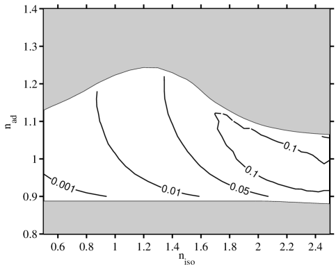
In Fig. 1 we show the allowed region in the ($n_{\rm iso}$,$n_{\rm ad}$)-plane, and the best-fit values of $\alpha$ for each ($n_{\rm iso}$,$n_{\rm ad}$). In Fig. 2 we show the allowed region ($\Delta\chi^{2}\leq 3.5$) in the ($n_{\rm iso}$,$n_{\rm ad}$,$\alpha$)-space as contours of maximum $\alpha$ on the ($n_{\rm iso}$,$n_{\rm ad}$) plane. This indicates the magnitude of the isocurvature contribution which remains allowed by the present data for different spectral indices.

FIG. 1.: The 68% (white), 95% (light gray), and 99.7% (medium gray) confidence level regions ($\Delta\chi^{2}=2.3$, 6.2, and 11.8) on the ($n_{\rm iso}$,$n_{\rm ad}$)-plane, and the best-fit values of $\alpha$ for each ($n_{\rm iso}$,$n_{\rm ad}$). The best-fit model (model 3) is marked with an asterisk ($\ast$).

FIG. 2.: The 68% confidence level region ($\Delta\chi^{2}\leq 3.5$) in the ($n_{\rm iso}$,$n_{\rm ad}$,$\alpha$)-space represented by contours of maximum $\alpha$. We do not show minimum $\alpha$, except that we show the region (between the dotted lines) where the minimum is $\alpha=0$.

FIG. 3.: Same as Fig. 2, but for $\alpha_{200}$.

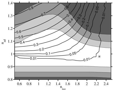
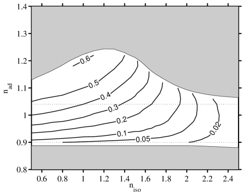
We see that a blue tilt, $n_{\rm ad}>1$, in the adiabatic spectrum favors a larger isocurvature contribution, since the low-multipole power from the isocurvature perturbations compensates for this tilt. In fact, the presence of an isocurvature contribution makes a larger $n_{\rm ad}$ acceptable than in the pure adiabatic case. A large blue tilt, $n_{\rm iso}\gg 1$, in the isocurvature spectrum makes it less helpful for this purpose, and the upper limit to $\alpha$ goes down again.

Since $\alpha$ measures the contribution to the lowest multipoles, the contribution to high multipoles for a given $\alpha$ is larger for large $n_{\rm iso}$. Thus, although the limits to $\alpha$ are tighter for large $n_{\rm iso}$, this does not mean that the contribution to high multipoles would have to be less. In fact, the largest allowed $\alpha_{200}$, above 0.1, are for spectral indices $n_{\rm iso}>1.8$ (see Fig. 3).

In Fig. 4 we show the angular power spectra for some of the models discussed above, together with the COBE, Boomerang, and Maxima-1 data. Figures 5 and 6 show separately the adiabatic and isocurvature contributions in models 5 and 6, which have large isocurvature contributions (large $\alpha$ and large $\alpha_{200}$, respectively) but are allowed by the present CMB data.

FIG. 4.: The data points of COBE ($\diamond$), Boomerang ($\bullet$), and Maxima-1 ($\circ$), and the angular power spectra of five models: (a) Our best-fit mixed (adiabatic+isocurvature) model (model 3, the solid line with the maximum at $l\sim 200$). (b) The best fit adiabatic model (model 1, dashed). (c) The best-fit isocurvature model (model 2, the solid line with the maximum at $l\sim 300$). (d) A mixed model with the largest ($\Delta\chi^{2}=4$) allowed $\alpha=0.63$ (model 5, dot-dashed). (e) A mixed model with the largest allowed $\alpha_{200}=0.13$ (model 6, dotted).

FIG. 5.: The angular power spectrum, $C_{l}$, and the adiabatic (dashed) and isocurvature (dot-dashed) contributions to it, $C_{l}^{\rm ad}$ and $C_{l}^{\rm iso}$, for model 5 with $(n_{\rm ad},n_{\rm iso})=(1.20,0.90)$ and $\alpha=0.63$.

FIG. 6.: Same as Fig. 5, but for model 6 with $(n_{\rm ad},n_{\rm iso})=(1.00,2.06)$ and $\alpha_{200}=0.13$.

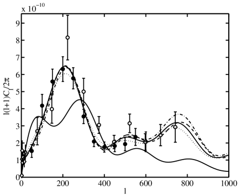
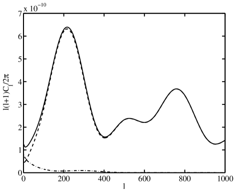
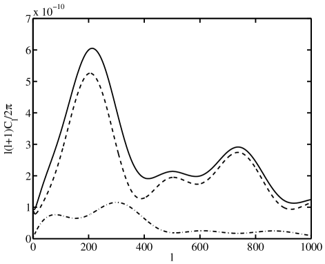
We see how the isocurvature contribution slightly modifies the shape of the angular power spectrum. In model 6 it fills the minima between the peaks in the adiabatic contribution. An isocurvature contribution with a large blue tilt could be the reason for the lack of prominence of the 2nd peak in the Boomerang data.

The Boomerang and Maxima teams estimate a calibration uncertainty of 10% and 4%, respectively, in their measurements. This uncertainty is not included in the above results. To study its effect, we multiplied the Boomerang measurements by $1.1^{2}$ and divided the Maxima-1 measurements by $1.04^{2}$. This brings the measurements closer to each other, since the Maxima-1 points tend to lie above the Boomerang points, with the exception of the $\l_{\rm eff}=147$ point. The best-fit mixed model becomes $n_{\rm ad}=1.00$, $n_{\rm iso}=1.78$, and $\alpha=0.05$ (model 9), with an improved fit, $\chi^{2}=20.9$. The upper limit to the isocurvature contribution is tightened to $\alpha\leq 0.56$ ($\alpha_{200}\leq 0.13$ stays the same), but the results do not change qualitatively.

The data is consistent with a purely adiabatic perturbation with $n_{\rm ad}\approx 1$, with the best fit $n_{\rm ad}$ = 0.96 (allowing for reionization would shift this even closer to 1). In large-field inflation models this translates into $r\lesssim 0.3$, so that the tensor contribution could be of the same order as the isocurvature contribution. Because of the degeneracy between isocurvature and tensor perturbation such a situation is not altogether surprising.

The COBE data together with $\sigma_{8}$ have an important role in constraining the spectral indices of the models. The Boomerang and Maxima-1 data are important in constraining the amplitude of the isocurvature contribution, as they outline the pattern of acoustic peaks and thus are able to distinguish between the different patterns of peaks[34] in the isocurvature vs adiabatic models.

V Conclusions

The main conclusion of the present work is that the Boomerang and Maxima-1 data definitely rule out all purely isocurvature models, including those with a large tilt [20, 21]. This is because Boomerang and Maxima-1 define the shape of the angular power spectrum in the region of the first acoustic peaks much more accurately than the previous data.

However, a significant isocurvature contribution remains allowed. Indeed, as much as about half of the power at low multipoles could come from the isocurvature contribution, although the adiabatic contribution must dominate the first acoustic peak. This certainly leaves much room for various particle physics models. We should however point out that in many models, such as two-field inflation models or Affleck-Dine models, isocurvature and adiabatic fluctuations are not completely independent, and much more stringent constraints on $\alpha$ (and possibly $n_{\rm iso}$) could be obtained in specific cases.

Note also that we cannot obtain any clear conclusion about the spectral index $n_{\rm iso}$; except for large $n_{\rm iso}$, the correlation between $\alpha$ and $n_{\rm iso}$ is small. MAP and Planck will provide new accurate data on high multipoles and therefore could further constrain $n_{\rm iso}$, but at moderate tilts we do not expect MAP to improve much on the Boomerang and Maxima-1 limit on $\alpha$. The situation with Planck is different, provided that high quality polarization data is achieved as expected. Polarization will resolve the degeneracy between isocurvature and tensor perturbations and push the limit on $\alpha$ lower by an order of magnitude [22]. Nevertheless, as discussed in the present paper, already the balloon experiments on the temperature fluctuations of the microwave sky can yield interesting constraints on particle physics models.