Optimal Supernova Search Strategies

Abstract

Recent use of Type Ia supernovae to measure acceleration of the universe has motivated questions regarding their optimal use to constrain cosmological parameters $\Omega_{M}$, $\Omega_{\Lambda}$ and $w_{Q}$. In this work we address the question: what is the optimal distribution of supernovae in redshift in order to best constrain the cosmological parameters? The solution to this problem is not only of theoretical interest, but can be useful in planning supernova searches. Using the Fisher matrix formalism we show that the error ellipsoid corresponding to $N$ parameters (for $N=1,2,3$) has the smallest volume if the supernovae are located at $N$ discrete redshifts, with equal number of supernovae at each redshift and with one redshift always being the maximum one probed. Including marginalization over the “nuisance parameter” $\mathcal{M}$ changes this result only trivially.

1 Introduction

Recent use of Type Ia supernovae (SNe Ia) as standard candles perlmutter-1997 ; perlmutter-1999 ; schmidt ; riess provided an opportunity to obtain the distance-redshift relation – and measure the cosmological parameters – without recourse to the “distance ladder”. SNe Ia provide strong evidence for the acceleration of the universe, thus implying that a component called “dark energy” with strongly negative pressure ($p<-1/3\,\rho$) dominates the energy-density of the universe. The most likely candidate for the dark energy is the vacuum energy, with $p=-\rho$. SNe Ia provide the luminosity distance – redshift relation and thus effectively determine the parameters $\Omega_{M}$ and $\Omega_{\Lambda}$, energy densities in matter and vacuum energy scaled to the critical energy density. The best-fit value using the current dataset of $\sim 50$ SNe Ia and assuming a flat universe is $\Omega_{M}=1-\Omega_{\Lambda}\simeq 0.3$, with $1$-$\sigma$ error of order $0.1$.

Given the importance of SNe Ia as standard candles — namely, determining the contents of the universe and probing the dark energy — it is important to consider what can be done to improve upon the constraints on cosmological parameters. Two obvious improvements would be increasing the size of the supernova sample and better control over the systematic errors. Going to redshifts beyond one is also very high on supernova cosmologists’ wish list because that way one can differentiate between the effects of dust and dark energy. It is believed that, barring unusual scenarios, dust would make faraway objects progressively fainter, while the dark energy becomes inoperative at $z>1$ because the universe is essentially matter-dominated at those redshifts. Finally, an important requirement would be to have supernovae located throughout the probed redshift range, in order to make sure that the magnitude-redshift relation traced out corresponds to the dark energy, and not evolution or dust. The planned supernova space telescope, SNAP snap-page , would satisfy all of the above-mentioned requirements.

This work considers supernova search strategies for the most accurate determination of cosmological parameters $\Omega_{M}$ and $\Omega_{\Lambda}$ (and possibly the equation of state ratio of the dark energy, $w_{Q}$, where ’Q’ stands for ’quintessence’ quint ). To this end, we ask: given the cosmological parameters we want to determine, what is the optimal distribution of supernovae in redshift in order to best constrain those parameters? At first glance this problem may appear of purely academic interest since we are not free to put supernovae where we please. However, supernova observers have considerable freedom in choosing redshift ranges for their searches, by using filters sensitive to wavelengths corresponding to spectra at observed redshifts. Moreover, the increased difficulty in observing high-redshift supernovae means that, even with great improvement in supernova detection and follow-up techniques, it can be as time-consuming to observe one supernova at, say, $z=1.4$ as many $z<1$ supernovae. Hence, an observer will have to decide how much telescope time is to be allocated to specific redshift ranges to best constrain the cosmological parameters.

In this work we make three assumptions:

$\bullet$ Magnitude uncertainty, $\sigma_{m}$, is the same for each supernova irrespective of redshift (this is a pretty good approximation, at least for current data sets).

$\bullet$ Total number of observed supernovae is fixed (rather than the total observing time, for example).

$\bullet$ There is an unlimited number of supernovae at each redshift.

None of these assumptions is required to use the formalism we present. Moreover, the results we present should qualitatively not be very different from those obtained when the constraints above are relaxed. We make the assumptions above to illustrate our approach and simplify the analysis.

2 The Most Accurate Parameter Determination

We tackle the following problem: given $n$ supernovae and their corresponding uncertainties, what distribution of these supernovae in redshift would enable the most accurate determination of cosmological parameters? In case of more than one parameter, we need to define what we mean by most accurate determination of all parameters simultaneously. Since the uncertainty in measuring $N$ parameters simultaneously is described by an $N$-dimensional ellipsoid (at least under assumption that the total likelihood function is gaussian), we make a fairly obvious and, as it turns out, mathematically tractable requirement that the ellipsoid have minimal volume. This requirement corresponds to the best local determination of the parameters.

We now show that volume of the ellipsoid is given by

$$V\propto\det(F)^{-1/2},$$ (1)

where the sign of proportionality expresses our ignorance of a numerical factor, and $F$ is the Fisher matrix Fisher-Jungman ; Fisher-Tegmark

$$F_{ij}=-\left<\partial^{2}\ln L\over\partial p_{i}\partial p_{j}\right>_{\bf y},$$ (2)

where $L$ is the likelihood of observing data set ${\bf y}$ given the parameters $p_{1}\ldots p_{N}$. Although this relation might be familiar/obvious to mathematically inclined cosmologists, we present its derivation for completeness.

To prove equation (1), consider a general uncertainty ellipsoid in $n$-dimensional parameter space. The equation of this ellipsoid is

$$X^{T}FX=1,$$ (3)

where $X=(x_{1}x_{2}\ldots x_{N})$ is the vector of coordinates and $F$ the Fisher matrix. Let us now rotate the ellipsoid so that all of its axes are parallel to coordinate axes. Equivalently we can rotate the coordinates to achieve the same effect, by writing $X_{\rm rot}=UX$, where $U$ is the orthogonal matrix corresponding to this rotation. The equation of the ellipsoid in the new coordinate system is

$$X_{\rm rot}^{T}\,F\,X_{\rm rot}=1,$$ (4)

or equivalently, in the original coordinate system

$$X^{T}\,F_{\rm rot}\,X=1,$$ (5)

where $F_{\rm rot}=U^{T}FU$ is the Fisher matrix for the rotated ellipsoid, and has the form $F_{\rm par}=diag(1/\sigma_{1}^{2},\ldots,1/\sigma_{N}^{2})$ with $\sigma_{i}$ the i-th axis of the ellipsoid. The volume of the (rotated) ellipsoid is obviously

$$V\propto\prod_{i=1}^{N}\sigma_{i}=\det(F_{\rm rot})^{-1/2}.$$ (6)

Then, since $\det(F)=\det(F_{\rm rot})$ and rotations preserve volumes, we have

$$V\propto\det(F_{\rm rot})^{-1/2}=\det(F)^{-1/2},$$ (7)

and this completes the proof.

2.1 Fisher Matrix for Supernovae

To minimize the volume of the ellipsoid we therefore need to maximize $\det(F)$. Fisher matrix for the case of supernova measurements was first worked out by Tegmark et al. CMB+SN , and we briefly recapitulate their results, with slightly different notation and one addition. The measurements are given as

$$m_{n}=5\log\;[H_{0}d_{L}(z_{n},\Omega_{M},\Omega_{\Lambda})]+{\mathcal{M}}+\epsilon_{n},$$ (8)

where $m_{n}$ is apparent magnitude of the $n$th supernova in the sample, $d_{L}$ is its luminosity distance, ${\mathcal{M}}\equiv M-5\log(H_{0})+25$ perlmutter-1999 (with $M$ absolute magnitude of a supernova), and $\epsilon_{n}$ is the error in that measurement (assumed to be drawn from a gaussian distribution with zero mean and standard deviation $\sigma_{m}$). Note that ${\mathcal{M}}$ contains all dependence on $H_{0}$, since $d_{L}\propto 1/H_{0}$.

The Fisher matrix is given by CMB+SN

$$F_{ij}=\frac{1}{\sigma_{m}^{2}}\sum_{n=1}^{N}w_{i}(z_{n})w_{j}(z_{n})$$ (9)

where $w$’s are weight functions given by

$$w_{i}(z)\equiv{5\over\ln 10}\left\{{\kappa S^{\prime}[\kappa I(z)]\over S[\kappa I(z)]}\left[{\partial I\over\partial p_{i}}-{I(z)\over 2\kappa^{2}}\right]+{1\over 2\kappa^{2}}\right\},$$ (10)

if the parameter $p_{i}$ is $\Omega_{M}$ or $\Omega_{\Lambda}$ (or $\Omega_{Q}$), or else

$$w_{i}(z)\equiv{5\over\ln 10}\left[{\kappa S^{\prime}[\kappa I(z)]\over S[\kappa I(z)]}\,{\partial I\over\partial p_{i}}\right]$$ (11)

if $p_{i}$ is $w_{Q}$. Also

$$H_{0}\,d_{L}=(1+z)\,\frac{S(\kappa I)}{\kappa},$$ (12)

$$S(x)=\left\{\begin{array}[]{cl}\sinh(x),&\;\mbox{if}\;\;\Omega_{\rm TOT}>1;\\ {x},&\;\mbox{if}\;\;\Omega_{\rm TOT}=1;\\ \sin(x),&\;\mbox{if}\;\;\Omega_{\rm TOT}<1.\end{array}\right.$$ (13)

$$I(z,\Omega_{M},\Omega_{\Lambda}) = \int_{0}^{z}A(z^{\prime})^{-1/2}dz^{\prime}$$ (14)

$$A(z) = \Omega_{M}(1+z)^{3}+\Omega_{\Lambda}+\kappa^{2}(1+z)^{2}$$ (15)

$$\kappa^{2} = 1-\Omega_{M}-\Omega_{\Lambda}.$$ (16)

Here $\Omega_{M}$, $\Omega_{\Lambda}$ and $\kappa^{2}$ are the energy densities in matter, cosmological constant and curvature respectively divided by the critical density, and $\Omega_{\rm TOT}\equiv\Omega_{M}+\Omega_{\Lambda}$. Later on we also consider a more general equation of state for the exotic energy, and replace the second term in equation (15) by $\Omega_{Q}(1+z)^{3(1+w_{Q})}$.

In addition to $\Omega_{M}$, $\Omega_{Q}$ and $w_{Q}$, the magnitude-redshift relation also includes the “nuisance parameter” $\mathcal{M}$, which is a combination of the Hubble parameter and absolute magnitude of supernovae, and which has to be marginalized over in order to obtain constraints on parameters of interest. Ignoring $\mathcal{M}$ in the Fisher matrix formalism (that is, assuming that $\mathcal{M}$ is known) leads to a serious underestimate of the uncertainties in other parameters (of course, fairly accurate knowledge of $H_{0}$ could be used to obtain $M$ from a sample of nearby supernovae, and thus determine $\mathcal{M}$). We continue to ignore $\mathcal{M}$ for simplicity and mathematical clarity, and in section 3.4 we show that including marginalization over $\mathcal{M}$ changes our results rather trivially.

The Fisher matrix can further be written as

$$F_{ij} = {N\over\sigma_{m}^{2}}\int_{0}^{z_{\rm max}}g(z)w_{i}(z)w_{j}(z)dz,$$ (17)

where

$$g(z)={1\over N}\sum_{n=1}^{N}\delta(z-z_{n})$$ (18)

is the (normalized) distribution of redshifts of the data and $z_{\rm max}$ is the highest redshift probed in the survey. Our goal is to find $g(z)$ such that $\det(F)$ is maximal. $g(z)$ is essentially a histogram of supernovae normalized to have unit area. Note that the maximization of $\det(F)$ will not depend on $N$ and $\sigma_{m}$, so we drop them from further analysis. To consider a non-constant error $\sigma_{m}(z)$, one simply absorbs $\sigma_{m}(z)$ into the definition of weight functions $w(z)$.

3 Results

3.1 Determination of One Parameter

We first consider the trivial – but instructive – case of one parameter. Then we need to maximize $\int_{0}^{z_{\rm max}}g(z)\,w_{1}^{2}(z)\,dz$, subject to $\int_{0}^{z_{\rm max}}g(z)\,dz=1$ and $g(z)\geq 0$. It is quite obvious that the solution is a single delta function at the redshift where $w_{1}(z)$ has a maximum. For any given parameter $w_{1}(z)$ will have a maximum at $z_{\rm max}$ and that is where we want all our supernovae to be. This result is hardly surprising: we have a one-parameter family of curves $m(z)$, and the best way to distinguish between them is to have all measurements at the redshift where the curves differ the most, at $z_{\rm max}$.

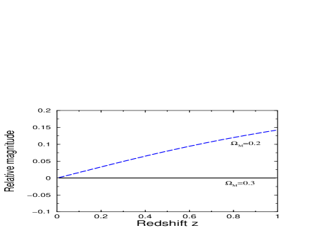
Figure 1: Dependence of the magnitude-redshift curve on a single cosmological parameter. We assume a flat universe and vary $\Omega_{M}=1-\Omega_{\Lambda}$. Magnitudes for the $\Omega_{M}=0.3$ flat model were subtracted from both curves for easier visualization

As an example, Fig. 1 shows magnitude-redshift curves for the fiducial $\Omega_{M}=0.3$ model with the assumption $\Omega_{\Lambda}=1-\Omega_{M}$ (flat universe). As $\Omega_{M}$ is varied, the biggest difference in $m(z)$ is at the highest redshift probed. In order to best constrain $\Omega_{M}$, therefore, all supernovae should ideally be located at $z=1.0$, our assumed maximum redshift.

3.2 Determination of Two Parameters

A more interesting – and relevant – problem is minimizing the area of the ellipse which describes the uncertainties for two parameters. The expression to maximize is then

$$\int_{z=0}^{z_{\rm max}}g(z)\,w_{1}^{2}(z)dz\int_{z=0}^{z_{\rm max}}g(z)\,w_{2}^{2}(z)dz\;-\left(\int_{z=0}^{z_{\rm max}}g(z)\,w_{1}(z)\,w_{2}(z)dz\right)^{2}$$ (19)

$$= {1\over 2}\int_{z_{1}=0}^{z_{\rm max}}\int_{z_{2}=0}^{z_{\rm max}}g(z_{1})\,g(z_{2})\,w^{2}(z_{1},z_{2})\,dz_{1}\,dz_{2},$$ (20)

where $w(z_{1},z_{2})\equiv w_{1}(z_{1})w_{2}(z_{2})-w_{1}(z_{2})w_{2}(z_{1})$ is a known function of redshifts and cosmological parameters (see Fig. 2) and $g(z)$ is subject to the same constraints as in case of one parameter.

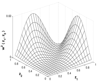
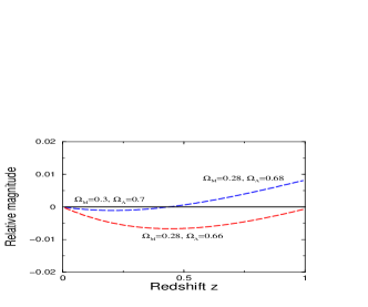
Figure 2: Left panel: Function $w^{2}{(z_{1},z_{2})}$ for the case when $\Omega_{M}=0.3$ and $\Omega_{\Lambda}=0.7$. Right panel: Variation of the magnitude-redshift curve when two cosmological parameters, $\Omega_{M}$ and $\Omega_{\Lambda}$, are varied independently

Despite a relatively harmless appearance of expression (20), we found it impossible to maximize it analytically. Fortunately, for all practical purposes numerical solution will be sufficient. Returning to the discretized version of equation (17), we divide the interval $(0,z_{\rm max})$ into $B$ bins with $g_{i}N$ supernovae in bin $i$. Then we need to maximize

$$\sum_{i,j=1}^{B}g_{i}\,g_{j}\,w^{2}(z_{i},z_{j})$$ (21)

subject to

$$\sum_{i=1}^{B}g_{i}=1\,\,\,\,\,\mbox{and}\,\,\,\,\ g_{i}\geq 0.$$ (22)

Equations (21) and (22) define a quadratic programming problem — extremization of a quadratic function subject to linear constraints. Since $w^{2}(z_{1},z_{2})$ is neither concave nor convex (see Fig. 2), we have to resort to brute force maximization, and consider all possible values of $g_{i}$. The result of this maximization is that the optimal distribution is two delta functions of equal magnitude:

$$g(z)=0.50\;\delta(z-0.43)+0.50\;\delta(z-1.00),$$ (23)

where all constants are accurate to $0.01$. Thus, half of the supernovae should be at the highest available redshift, while the other half at about 2/5 of the maximum redshift.

This result is not very sensitive to the maximum redshift probed, or fiducial parameter values. If we increase the maximum available redshift to $z_{\rm max}=1.5$, we find two delta functions of equal magnitude at $z=0.57$ and $z=1.50$. If we change the fiducial values of parameters to $\Omega_{M}=0.3$ and $\Omega_{\Lambda}=0$ (open universe), we find delta functions of equal magnitude at $z=0.47$ and $z=1.00$.

Finally, let us consider a different choice for the two parameters — for example, $\Omega_{M}$ and $w_{Q}$ (equation of state of the dark energy), with fiducial values $\Omega_{M}=0.3$ and $w_{Q}=-1$ and with the assumption of flat universe ($\Omega_{Q}=1-\Omega_{M}$). Then, assuming $z_{\rm max}=1.0$, we get

$$g(z)=0.50\;\delta(z-0.36)+0.50\;\delta(z-1.00),$$ (24)

and again optimal distribution of supernovae is similar to the case of $\Omega_{M}$ and $\Omega_{\Lambda}$ as parameters.

3.3 Determination of Three Parameters

We further consider parameter determination with three parameters $\Omega_{M}$, $\Omega_{Q}$ and $w$. Elements of the 3x3 Fisher matrix are calculated according to expression (17), and we again maximize $\det(F)$ as described above. The result is

$$g(z) = 0.33\;\delta(z-0.21)+0.34\;\delta(z-0.64)+$$ (26)

$$0.33\;\delta(z-1.00),$$

with all constants accurate to 0.01. Hence we have three delta functions of equal magnitude, with one of them at the highest available redshift.

It appears impossible to prove that $N$ parameters are best measured if the data form $N$ delta functions in redshift. However, it is easy to prove that, if the data do form $N$ delta functions, then those delta functions should be of equal magnitude and their locations should be at coordinates where the “total” weight function (e.g. $w^{2}(z_{1},z_{2})$ in case of two parameters) has a global maximum. In practice, the relevant number of cosmological parameters to be determined from the SNe Ia data is between one and three, so considering more than three parameters is less relevant for practical purposes.

3.4 Including Marginalization over $\mathcal{M}$

So far we have been ignoring the parameter $\mathcal{M}$, assuming that it is known (equivalently, that the value of $H_{0}$ and the absolute magnitude of supernovae are precisely known). This, of course, is not the case, and $\mathcal{M}$ is marginalized over to obtain probabilities on cosmological parameters. Fortunately, when $\mathcal{M}$ is properly included, our results change in a predictable and rather trivial way, as we now show.

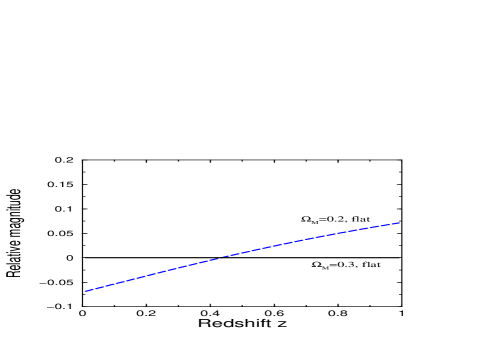
Figure 3: Magnitude-redshift curve when a single cosmological parameter, $\Omega_{M}$, is varied. Marginalization over $\mathcal{M}$ is now included, which means that the curves are allowed to slide vertically as well

Including $\mathcal{M}$ as an undetermined parameter, we now have an $N+1$-dimensional ellipsoid ($N$ cosmological parameters plus $\mathcal{M}$), and we want to minimize the volume of its projection onto the $N$-dimensional space of cosmological parameters. The equation of the $N$-dimensional projection is

$$X^{T}F_{\rm proj}X=1$$ (27)

and $F_{\rm proj}$ is obtained as follows: 1) Invert the original $F$ to obtain the covariance matrix $F^{-1}$  2) pick the desired $N$x$N$ subset of $F^{-1}$ and call it $F_{\rm proj}^{-1}$, and   3) invert it to get $F_{\rm proj}$.

Minimizing the volume of the projected ellipsoid we obtain the result that the optimal supernova distribution is obtained with $N$ delta functions in redshift obtained when ignoring $\mathcal{M}$, plus the delta function at $z=0$. All $N+1$ delta functions have the same magnitude. The intuitive explanation for this result is illustrated in Fig. 3, which shows the magnitude-redshift curves when $\Omega_{M}$ and $\mathcal{M}$ are varied (flat universe is assumed). This figure is the same as Fig. 1, except the curves are now allowed to slide vertically as well, corresponding to the variation in $\mathcal{M}$. There are two locations of largest departure when the two parameters are varied, namely $z=0$ and $z=1$. It makes sense then that those are precisely the locations where the supernovae should be, and our analysis says that we ideally need equal number of supernovae at each location.

3.5 Optimal vs Uniform Distribution

Are the advantages of the optimal distribution significant enough that one should consider them seriously? In our opinion the answer is affirmative, as we illustrate in the left panel of Fig. 4. This figure shows that the area of the $\Omega_{M}$-$\Omega_{\Lambda}$ uncertainty ellipsoid is more than two times smaller if the SNe have the optimal distribution in redshift as opposed to the case of uniform distribution.

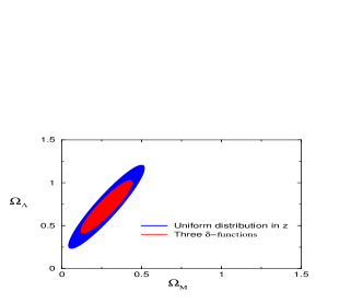
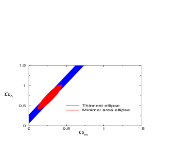
Figure 4: Left panel: Uniform (dark-blue) vs optimal (light-red) distribution in redshift. Shown are constraints on $\Omega_{M}$ and $\Omega_{\Lambda}$ when $\mathcal{M}$ was marginalized over. To get the absolute sizes of the ellipses, $N=100$ SNe were assumed with individual uncertainties of $\sigma_{m}=0.15$ mag. Right panel: Thinnest possible ellipse for given $N$ and $\sigma_{m}$ (dark-blue) is infinitely long in one direction. However, the smallest-area ellipse (light-red) is almost as thin, and for all purposes can serve as the thinnest ellipse

3.6 Requiring the Thinnest Ellipse

If we are using SNe Ia alone to determine the cosmological parameters, then we clearly want to minimize the area of the error ellipse (we consider the case of $\Omega_{M}$ and $\Omega_{\Lambda}$ as parameters in this section). However, supernova measurements will also be combined with other methods to determine the parameters. A prime example of a symbiosis between two or more methods is combining CMB measurements with those of supernovae Zaldarriaga ; CMB+SN . These methods together can improve the determination of $\Omega_{M}$ and $\Omega_{\Lambda}$ up to a factor of 10 as compared to either method alone due to breaking of the degeneracy between the two parameters. As can be seen in Fig. 2 of ref. CMB+SN , in combining the CMB with SNe Ia data one might hope for the thinnest ellipse possible coming from supernova measurements. Here by “thin” we mean that the combination $\Omega_{M}-\Omega_{\Lambda}$ is accurately determined.

Finding the thinnest ellipse is the problem that we can solve using our formalism, since the length of each axis of the ellipse is proportional to the inverse square root of an eigenvalue of the corresponding Fisher matrix. All we need to do then is maximize the larger eigenvalue of $F$ with respect to the distribution of the supernovae $g(z)$.

The result is perhaps not at all surprising: to get the thinnest ellipse, all supernova measurements should be at the same (maximum) redshift, which at the same time implies an infinitely long ellipse. More generally, we find that changing the redshift distribution of supernovae doesn’t change the thickness of the error ellipse greatly, but does change its length. By attempting to obtain a thinner ellipse, we end up only making it longer. Fortunately, the smallest area ellipse we found can in practice serve as the thinnest ellipse, as shown in the right panel of Fig. 4.

3.7 Reconstruction of the Potential of Quintessence

It has been shown recently that a sufficiently good supernova sample could be used to reconstruct the potential of quintessence out to $z\simeq 1$ reconstr ; chiba . More generally, equation of state ratio of the missing energy, $w_{Q}$, can also be reconstructed reconstr .

In the spirit of our analyses above, we ask: what distribution of supernovae in redshift gives the smallest 95% confidence region for the reconstructed potential $V(\phi)$? To answer this question, we perform a Monte-Carlo simulation by using different distributions of supernovae and computing the average area of the confidence region corresponding to each of them.

Uniform distribution of supernovae gives the best result among the several distributions we put to test. This is not surprising, because reconstruction of the potential consists in taking first and second derivatives of the distance-redshift curve, and the most accurate derivatives are obtained if the points are distributed uniformly. For comparison, gaussian distribution of supernovae with $\overline{z}=0.7,\sigma_{z}=0.4$ gives the area that is $10-20$% larger.

4 Discussion

We considered supernova search strategies that produce the tightest constraint on cosmological parameters by minimizing the volume of the error ellipsoid corresponding to those parameters. We first proved that, assuming that the total likelihood function is gaussian, the volume of an $N$-dimensional error ellipsoid is proportional to the inverse square root of the determinant of the corresponding Fisher matrix. Then we showed that, if the supernova measurements are used to determine $N$ parameters with $N=1,2$ or $3$, this volume is minimized if the distribution of supernovae in redshift is given by $N$ delta functions of equal magnitude. In particular, $\Omega_{M}$ and $\Omega_{\Lambda}$ have the smallest error ellipse if half of the measurements are at $z_{\rm max}$, while the other half are at roughly $2/5\,z_{\rm max}$. If $\mathcal{M}$ is marginalized over, we need an additional supernova sample at $z=0$ (a total of $N+1$ delta functions in redshift).

Our approach is quite flexible and can be applied in practice. For example, given the redshift-dependence of the measurement uncertainties for a given experiment, $\sigma_{m}(z)$, as well as the time it takes to obtain a measurement at a given redshift (determined by the telescope specifications), one can perform analysis similar to that in section 3 to infer the optimal search strategy.

It is important to keep in mind that the best determination of the parameters around their fiducial values is only one of the possible objectives. As mentioned in the introduction, tracing out the magnitude-redshift curve throughout the redshift range is important to test for systematics such as evolution or dust. A sample of nearby supernovae would be useful to further check for systematics (at least one low-z SN search program is already under way). Ultimately, the chosen supernova search strategy should combine all of these considerations.

Acknowledgments.

We would like to thank members of the Supernova Cosmology Project and Daniel Holz for useful discussions. This work was supported by the DoE (at Chicago and Fermilab) and by the NASA (at Fermilab by grant NAG 5-7092).

References

- (1) S. Perlmutter et al: Astrophys. J. 483, 565 (1997)
- (2) S. Perlmutter et al: Astrophys. J. 517, 565 (1999)
- (3) B. Schmidt et al: Astophys. J. 507, 46 (1998)
- (4) A. Riess et al: Astron. J. 116, 1009 (1998)
- (5) M. Phillips: Astrophys. J. 413, 108 (1993)
- (6) G. Jungman et al: Phys. Rev. D 54, 1332 (1996)
- (7) M. Tegmark, A. N. Taylor, A. F. Heavens: Astrophys. J. 480, 22 (1997)
- (8) M. Tegmark et al, ’Cosmic Complementarity: Probing the Acceleration of the Universe’, astro-ph/9805117
- (9) http://snap.lbl.gov
- (10) R. Caldwell, R. Dave, P.J. Steinhardt: Phys. Rev. Lett. 80, 1582 (1998)
- (11) J. C. G. Boot: Quadratic Programming: Algorithms, Anomalies [and] Applications (North-Holland Pub. Co., Amsterdam 1964)
- (12) M. Zaldarriaga, D. N. Spergel, U. Seljak: Astrophys. J. 488, 1 (1997)
- (13) D. Eisenstein, W. Hu, M. Tegmark: Astrophys. J. 518, 2 (1999)
- (14) D. Huterer, M.S. Turner: Phys. Rev. D 60, 081301 (1999)
- (15) T. Nakamura, T. Chiba: Mon. Not. Roy. Astron. Soc. 306, 696 (1999)