The Synthesis Telescope at the Dominion Radio Astrophysical Observatory

Abstract

We describe an aperture synthesis radio telescope optimized for studies of the Galactic interstellar medium (ISM), providing the ability to image extended structures with high angular resolution over wide fields. The telescope produces images of atomic hydrogen emission using the 21-cm H i spectral line, and, simultaneously, continuum emission in two bands centred at 1420 MHz and 408 MHz, including linearly polarized emission at 1420 MHz, with synthesized beams of $1^{\prime}$ and $3.4^{\prime}$ at the respective frequencies. A full synthesis can achieve a continuum sensitivity (rms) of 0.28 mJy/beam at 1420 MHz and 3.8 mJy /beam at 408 MHz, and the 256-channel H i spectrometer has an rms sensitivity of 3.5$B^{-0.5}\sin\delta$ K per channel, for total spectrometer bandwidth $B$ MHz and declination $\delta$. The tuning range of the telescope permits studies of Galactic and nearby extragalactic objects. The array uses 9 m antennas, which provide very wide fields of view of 3.1° and 9.6° (at the 10% level), at the two frequencies, and also allow data to be gathered on short baselines, yielding extremely good sensitivity to extended structure. Single-antenna data are also routinely incorporated into images to ensure complete coverage of emission on all angular scales down to the resolution limit. In this paper we describe the telescope and its receiver and correlator systems in detail, together with calibration and observing strategies that make this instrument an efficient survey machine.

1 Introduction

The Synthesis Telescope at the Dominion Radio Astrophysical Observatory (DRAO) is a radio telescope with unique capabilities for Galactic interstellar medium (ISM) studies. Operating simultaneously at the frequency of the spin-flip spectral line of atomic hydrogen (the H i line near 1420 MHz), and in two continuum bands near 1420 MHz and 408 MHz, the telescope achieves arcminute angular resolution with exceptional sensitivity to extended structure over wide fields (3.12° at 1420 MHz and 9.63° at 408 MHz at the 10% level). These features allow it to map several major constituents of the ISM, namely the atomic gas (through the H i line), the ionized gas (thermal continuum emission detected in the continuum bands), and the relativistic component (which generates synchrotron emission, measured in the continuum bands) in a way which few other telescopes can match. Its principal project at the time of writing is the Canadian Galactic Plane Survey (Taylor et al. (2000)); data from this survey are now entering the public domain. The purpose of this paper is to acquaint the scientific community with the characteristics of the telescope.

The telescope in its original form was described by Roger et al. (Roger73 (1973)), with the first astronomical results being published shortly thereafter (Costain et al. (1976); Roger & Costain 1976). Over the following two decades the capabilities of the telescope were enhanced through a series of modifications, including increasing the number of antennas from 2 to 4 and doubling the maximum baseline in 1982, adding a 408 MHz continuum channel in 1984, and adding a second receiver path to the 1420 MHz continuum system in 1986 to allow both hands of circular polarization (CP) to be measured.

An extensive rebuilding of the telescope began in 1992, to create a telescope optimized for studies of the Galactic ISM, concentrating on high angular resolution, wide-field studies of H i. Enhancements over the following 3 years included the addition of three antennas, a new 1420 MHz continuum correlator with double the reception bandwidth and polarimetry capabilities, and a new H i spectrometer with double the number of channels. The result is a substantially new telescope, built on the basic infrastructure of the old. In this paper we describe the telescope, with emphasis on its new components.

2 Array design

2.1 Basic design objectives

The telescope was conceived as a tool for the study of the Galactic H i, which is known to have structure on all angular scales at which observations have been attempted, from tens of degrees (Hartmann & Burton (1997)) to tens of milli-arcseconds (Faison et al. (1999)). An angular resolution of 1 arcmin was the target, an order of magnitude improvement over the resolution available with the largest single-antenna radiotelescopes, while retaining sensitivity to intermediate and larger structures. This required a finely sampled aperture plane and short interferometer baselines, which in turn dictated the use of small antennas. It was also clear at the outset that it would be necessary to incorporate single-antenna data into the Synthesis Telescope images (see §2.3) and to mosaic individual images together to extend the field of view.

A telescope which can successfully image H i emission will also be suitable for imaging Galactic continuum emission, which similarly displays a wide range of structural sizes. Continuum emission at decimetre wavelengths originates in the ionized and relativistic components of the ISM. The latter gives rise to a small percentage of linear polarization in the emission, and the ability to measure polarization was included in the telescope to give information on magnetic fields at the point of origin and on the magneto-ionic medium along the line of sight.

With only seven antennas, the number of instantaneous baselines is just 21; many more baselines are required to meet the desired imaging criteria. The chosen configuration was therefore an east-west aperture synthesis telescope with movable elements. Earth rotation varies the baseline vector during an observation, and the movable antennas are relocated until the required set of baselines has been completely sampled in consecutive observations. (The normal observing strategy for the telescope is described in §8).

2.2 Array configuration

The task of designing an array configuration to meet the above objectives was constrained by the existing four-antenna array, which had two movable antennas on 300 m of rail, along with two fixed antennas, one at the west end of the rail and one $\sim 600$ m to the east. With the possibility of adding only three additional antennas, the final configuration (Figure 1) was dictated by the needs of both continuum and H i-line imaging described above.

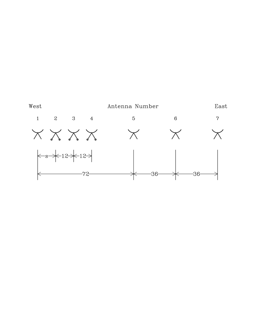
Figure 1: The telescope configuration. Antenna separations are shown in units of $L=4.286$ m. The separation, s, between antennas 1 and 2 varies from $3L$ to $14L$ as antennas 2, 3, and 4 are moved along a rail track.

The diameter of the antennas used in the array is 8.5 m (for further details see §3). The baseline increment is $L=4.286$ m, about half an antenna diameter. This provides the necessary fine baseline sampling, and places the first grating response at an angular radius where the primary beam of the antennas is at a very low level, so that grating responses to objects within the usable field of view lie outside the field (although responses to strong sources outside the usable field can still appear within it). Antenna shadowing and the risk of mechanical interference limit the minimum usable baseline to $3L\simeq 12.86$ m, which is sufficient to allow full representation in the images of structures as large as 40 arcmin at 1420 MHz and 2.3° at 408 MHz. A maximum baseline of $144L\simeq 617.1$ m provides the desired 1-arcmin resolution limit at 1420 MHz (at 408 MHz a resolution of 3.4 arcmin is achieved). Table 1 lists the telescope specifications.

Table 1: Telescope specifications

Operating frequencies:		1420 MHz
		408 MHz
Number of antennas:		7
Antenna diameter:		five 8.53 m, two 9.14 m
Maximum baseline:		617.18 m
Minimum baseline:		12.86 m
Baseline increment:		4.286 m
Visibility averaging time:		90 seconds
Field of view:	1420 MHz	2.65° diameter to 20%
	408 MHz	8.22° diameter to 20%
Angular resolution:	1420 MHz	$58^{\prime\prime}\times 58^{\prime\prime}$ cosec$\delta$
	408 MHz	$3.4^{\prime}\times 3.4^{\prime}$ cosec$\delta$
Radius of first grating ring:	1420 MHz	2.82°
	408 MHz	9.82°
Polarization imaging:	1420 MHz	Stokes $I$, $Q$, and $U$
	408 MHz	One hand of circular
		(usually RHCP)
System temperature:	1420 MHz	60 K
	408 MHz	105 K + $T_{sky}$
Continuum bandwidth:	1420 MHz	30 MHz
	408 MHz	3.5 MHz
Tuning range for H i:		$-$1100 to +3000 km s-1
Spectrometer frequency coverage ($B$):		0.125, 0.25, 0.5, 1.0, 2.0, 4.0 MHz
Number of spectrometer channels		256
Velocity coverage for H i:		211$B$ km s-1
Channel separation:		0.824$B$ km s-1
Channel width:		1.32$B$ km s-1
Noise on 1-channel spectral map:		$3.5B^{-0.5}\sin\delta$ K

The three movable antennas are mounted on motorized platforms that ride on a precise, machined track that is dimensionally stable and accurately surveyed. Station markers along the track are used in positioning the antennas, with a one-station move taking about 5 minutes. The antennas are usually moved so that they are $12L$ apart, with the separation between antennas 1 and 2 ($s$ in Fig. 1) ranging from $3L$ to $14L$. By this means, complete coverage of baselines from $3L$ to $141L$ (plus $144L$) is obtained with 12 settings of the movable antennas. The time required to synthesize a complete aperture is therefore $12\times 12$ hours. The telescope is almost always used in this mode. An exception is solar imaging (Burke & Tapping Burke95 (1995)); for this purpose a set of spacings has been selected which allows the formation of a satisfactory image of the Sun (in the absence of rapid variation such as burst activity) in one 12-hour observation.

For H i imaging, only the 12 baselines between the four fixed and three movable antennas are used. H i-line images are typically of limited dynamic range, determined by the ratio of the maximum brightness temperature (rarely more than 120 K) to the expected noise level ($\sim 3$ K). However, antenna-based calibration parameters, determined from continuum measurements using all 21 baselines, are routinely applied to H i visibilities.

2.3 Complementary single-antenna data

The short baselines available on the Synthesis Telescope permit accurate imaging of quite large features, but it is still necessary to incorporate data from single-antenna radio telescopes into the images. The DRAO 26-m Telescope is usually used to provide the necessary information on the largest H i structures. Single-antenna continuum data at 1420 MHz are obtained from the Effelsberg surveys of Kallas & Reich (Kallas80 (1980)), Reich et al. (Reich90 (1990)), and Reich et al. (Reich97 (1997)) or from the Stockert surveys of Reich (Reich82 (1982)) and Reich & Reich (Reich86 (1986)). When a long-wavelength channel was planned for the Synthesis Telescope in the 1980s, the frequency of 408 MHz was chosen because of the existence of a complementary, well-calibrated, single-antenna survey of the whole sky at that frequency (Haslam et al. (1982)).

3 Antennas

The antennas used in the Synthesis Telescope have equatorially mounted, paraboloidal reflectors. There are two slightly different designs in use, the most significant difference being that two antennas (at the east and west extremes of the array) have diameter $d=9.14$ m and focal length $f=3.81$ m ($f/d=0.42$), while the remainder have $d=8.53$ m and $f=3.66$ m ($f/d=0.43$). The difference in antenna diameters leads to a mismatched weighting of u-v samples which is sufficiently large to affect imaging; Willis (Willis99 (1999)) has devised a means of compensating for this effect.

Signals are collected by a dual-frequency feed (Veidt et al. Veidt85 (1985); Trikha et al. Trikha91 (1991)) mounted at the prime focus. Circular polarization (CP) is received at both frequencies: continuum emission is expected to have a small fraction of linear polarization (from synchrotron radiation), and measurement of that component can be made most simply by using CP feeds.

At 1420 MHz a multi-mode feed, based on one of the designs of Sheffer (Scheffer75 (1975)), provides a flat-topped illumination pattern, yielding an aperture efficiency $\eta_{A}=0.55$, with an edge illumination of the reflector of $-16$ dB. A “quarter-wave plate” in the waveguide (consisting of three reactive posts; Simmons (1952)) provides a 90° phase shift, and linear probes aligned at 45° to the plane of the quarter-wave plate collect left-hand circular polarization (LHCP) and right-hand circular polarization (RHCP) simultaneously.

The circularly polarized 408-MHz feed was added subsequently, and was designed to avoid any degradation of 1420-MHz performance. The outputs of four orthogonal monopoles, placed in the outer cavity of the 1420-MHz feed, are combined in a TEM-mode hybrid. A switch selects either LHCP or RHCP; normally RHCP is received (the use of a CP feed gives an accurate measurement of Stokes $I$ even in the presence of some linearly polarized emission). At 408 MHz the feed has the radiation characteristics of a circular waveguide of diameter $0.7\lambda$, illuminating the aperture very broadly. The aperture efficiency is $\eta_{A}=0.6$, but edge illumination is high ($-8$ dB) and beam efficiency is low ($\eta_{B}=0.70$) because of the high spillover.

Antenna noise temperature at 1420 MHz varies from a high of 26.0 K on one antenna to a low of 17.8 K on another, because of slight differences in construction. Table 2 gives details of the noise budgets of the best and worst antennas. These data were derived by Anderson et al. (Anderson91 (1991)) based on two-dimensional mapping of the radiation pattern of one of the antennas. The feed-support struts of several antennas have been modified (Landecker et al. Landecker91 (1991)) to reduce the ground noise which the struts scatter into the aperture.

Table 2: Antenna noise-temperature budget at 1420 MHz (K)

Cosmic microwave background	2.7
Galactic emission	1.0
Atmospheric emission (zenith)	2.0
Main beam contribution:	5.7
	Worst		Best
	antenna		antenna
Spillover	8.0		8.0
Diffraction at reflector rim	0.6		0.6
Mesh leakage	5.9		1.5
Strut scattering	5.8		2.0
Sidelobe contributions:	20.3		12.1
Total:	26.0		17.8

4 Receivers

4.1 The 1420-MHz receiver

Sensitivity at 1420 MHz is primarily determined by the low-noise HEMT amplifier, which has a noise temperature, $T_{R}\approx 35$ K (for 16 amplifiers built, 28 K $<T_{R}<38$ K and $\langle T_{R}\rangle=33.4$ K). The uncooled 3-stage amplifier is an enhanced version of the amplifier described by Walker et al. (Walker88 (1988)). It uses source-inductance feedback to achieve a good input match (Weinreb et al. Weinreb82 (1982)).

After filtering to suppress the image band, the signal is converted to an intermediate frequency (IF) band of 12.5–47.5 MHz. IF signals are conveyed from each antenna to the central building by coaxial cables. No compensation is attempted for changes in IF phase due to cable-length changes with temperature; physical matching of cables provides adequate stability.

The Local Oscillator (LO) system (Landecker & Vaneldik Landecker82 (1982)) delivers signals of controlled frequency and phase to the mixers at each antenna. To control phase, the system uses the “round-trip” design, in which the electrical length of the cable connecting the central electronics to the antenna is measured by sending a signal out to the antenna and back. If the cable electrical length changes by $\epsilon$, the returning signal changes its phase by the equivalent of $2\epsilon$. Closing the feedback loop requires a division by 2; consequently there is an ambiguity of $\pi$ in the output phase. This difficulty is overcome by operating the round-trip system at half the frequency of the required LO signal. At the antenna, the output is doubled to produce the LO signal near 1390 MHz. The tuning range of the LO system is given in Table 1; it accommodates observations of H i in the Galaxy and in nearby extragalactic systems.

The interferometer fringe rate is reduced to zero for each baseline by rotating the phase of the LO signal for each antenna relative to the reference antenna (Antenna 5 at the physical centre of the array – see Figure 1). Phase switching in a Walsh-function pattern (Granlund et al. Granlund78 (1978)) is also applied to the LO signal to reduce spurious correlation from crosstalk between receiver channels. The switching pattern has 16 steps of 5.6 s in the telescope visibility-averaging time of 90 s.

Compensating delays are inserted in the IF signal paths to equalize path lengths, from the incoming wavefront, through each antenna to the correlator. Stripline paths are used for short delays and coaxial cable for longer delays, selected by PIN diode switches. Cable delay sections are equalized for attenuation and dispersion. This is an enhancement of the earlier system described by Landecker (Landecker84 (1984)). The minimum delay step of 3.91 cm ($\approx 0.13$ ns) is determined by the specification that the delay error should produce a phase difference across the spectrometer band of less than 0.1°. Delay system specifications are given in Table 3.

Table 3: 1420 MHz delay system specifications

Delay medium:	stripline and coaxial cable
Frequency range:	10 to 50 MHz
Delay step:	$2^{-8}\lambda_{30}=3.91$ cm
Total delay:	$64\lambda_{30}=640$ m
Amplitude accuracy:	$\pm 0.02$ dB (rms)
Phase accuracy:	$\pm 1$°(rms)

Residual gain fluctuations due to imperfect delay-cable equalization or unequal switch losses are removed by an automatic gain control (AGC). The AGC measures signal levels at the delay-system input and output, and keeps the net gain of the delay system constant. A second gain monitor spans the entire signal path, from antenna feed to correlator output: small modulated noise signals ($\Delta T_{A}\approx 1$ K) are injected into each antenna feed, and are demodulated from autocorrelation outputs (see §5.1) to give continuous measurements of system gain and system temperature.

Since this is a spectroscopic telescope, the reception frequency must be varied to account for diurnal and orbital motion of the Earth, as well as for the radial velocity of the source under observation. The total reception band, of width 35 MHz, is kept centred on the H i band selected for observation by continuously tuning the first LO. The continuum reception band is divided into four sub-bands distributed on either side of the spectroscopy band, as illustrated in Figure 2. In the course of an observation, continuum band centres vary as the LO is tuned, but the imaging software accounts for this slight change. The five reception bands are translated to fixed locations in the IF band.

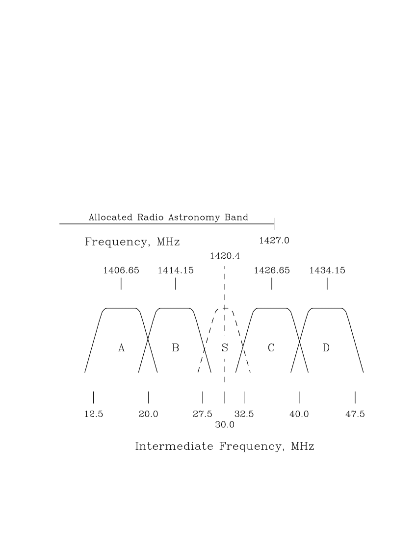
Figure 2: The arrangement of continuum and spectroscopy bands near 1420 MHz. S is the band used for H i spectroscopy, and A, B, C, and D are continuum bands. The system LO is varied to keep the H i information centred in the IF at 30.0 MHz. The band allocated to radio astronomy extends from 1400 to 1427 MHz; part of band C and all of band D are outside the protected band. The overall width of the spectroscopy band can be varied from 0.125 to 4 MHz (see text).

The four continuum bands are defined by IF bandpass filters and are converted to baseband using fixed second LOs. A quadrature replica of each band is created using a phase-shifted second LO. The spectrometer band is converted to lower frequency in a single-sideband mixer. The overall bandwidth of the spectrometer is selectable with six options from $B=0.125$ MHz to $B=4.0$ MHz in multiples of 2. Before digitizing, the band is sharply defined by a six-pole elliptic-function bandpass filter spanning $B$ to $2B$. Use of this “quasi-baseband” allows better image rejection in the single-sideband mixer.

4.2 The 408-MHz receiver

The 408 MHz receiver is designed to use as much as possible of the band assigned to radio astronomy (406.1–410 MHz), while suppressing out-of-band communications signals. Several stages of filtering are distributed between gain stages in the receiver, and a total bandwidth of 3.5 MHz is achieved.

A single coaxial cable carries both LO and IF signals between the focus of each antenna and the central receiver building. The LO phase is controlled by a feedback system which keeps the phase of the 30 MHz IF signal arriving at the centre of the telescope completely independent of the length of the interconnecting cable (Veidt et al. Veidt85 (1985)). All subsequent signal processing is carried out in digital electronics or in software (see §5.3). A minor drawback of the LO-IF system is the generation of an unwanted fixed-frequency signal at the centre of the IF band; this is removed prior to correlation by a narrow bandstop filter.

5 Correlators

The three operating bands of the telescope, the 1420-MHz continuum band, the H i spectroscopy band, and the 408-MHz continuum band, use digital correlators of different designs, which we label the C21, S21, and C74 systems respectively. The three correlators were built at different times; their design differences are partly dictated by that history but are mostly driven by the significantly different requirements. Table 4 lists the specifications of the three correlators.

Table 4: Correlator characteristics

Correlator	C21	S21	C74
Bandwidth (MHz)	7.5 ($\times 4$)	$2^{n}$, $-3\leq n\leq 2$	4.0∗
Sampling rate (MHz)	20.0	2$f_{N}^{\dagger}$	16.0
Correlator efficiency	0.985	0.88	0.88
Number of quantizer levels	14	3	3
∗ Bandwidth actually used is 3.5 MHz, defined by RF filters
${}^{\dagger}f_{N}=$ Nyquist frequency

Digital representation of signals introduces quantization noise, some of which can be recovered by increasing the sampling rate (Bowers & Klingler Bowers74 (1974); Klingler Klingler74 (1974)). Figure 3 shows correlator efficiency for the two quantization schemes used in this telescope.

Figure 3: Correlator efficiency. Curves (a) and (b) show the efficiency of a 3-level correlator at Nyquist and double-Nyquist sampling rates respectively, and (c) and (d) show the same for a 14-level correlator. The horizontal axis is labelled with the voltage setting of the first quantizer threshold in units of the r.m.s. value of the input signal. In each correlator on the telescope, the input signal level is chosen to optimize correlator efficiency.

Sections 5.1, 5.2 and 5.3 describe the three correlators in turn. Section 5.4 describes routines developed to correct the inherent correlator non-linearity. These corrections are currently applied to C21 and S21 data only.

5.1 The 1420-MHz continuum correlator

The C21 correlator (Karpa (1989)) uses fourteen-level representation of the input signals; with moderate over-sampling, it achieves an unusually high correlator efficiency ($\eta_{c}=0.985$; see Figure 3). The correlator was designed to provide products from all antenna pairs, and to form all four polarization products from the LHCP and RHCP inputs. However, the total continuum bandwidth is too wide to permit mapping of the entire field of view of the telescope without bandwidth smearing (decorrelation arising from differential delay of off-axis, wide-bandwidth signals; see Bridle & Schwab (1989)). The 30 MHz band is therefore divided into four 7.5 MHz sub-bands as illustrated in Figure 2. Each sub-band input is digitized to 14 levels and the products are formed in one of four identical correlators.

Input signals are digitized using four-bit monolithic flash converters (Analog Devices AD9688) with the sampling clock running at 20 MHz, slightly faster than the Nyquist rate for a 7.5-MHz bandwidth. Of the 16 possible A/D output levels, only 14 are used. The two extreme levels (outputs 0000 and 1111) are reserved for use as control signals embedded in the data stream.

Each correlator module uses a ROM look-up table where an 8-bit product is stored at the address specified by the two 4-bit inputs. The product is accumulated for 5.6 seconds. The occurrence of the code 0000 at either input of the multiplier causes accumulation to stop. The accumulator (a combination of synchronous and ripple counters) is allowed to settle, and is then read by the system microprocessor.

The occurrence of code 1111 on one of the multiplier inputs causes the multiplier to produce an 8-bit output corresponding to the square of the 4-bit number appearing on the other input. Extra correlator cards are used in this way as auto-correlators, and they generate outputs corresponding to the power in each input signal. Small noise signals are injected into each antenna (see §4.1), and the autocorrelation outputs are used to measure both system gain and noise in each channel. Additional correlator channels are used to compute the mean of each input signal (by multiplying the input signal by a fixed number), a measure of the error in each A/D converter. Similarly, “self-correlations” are formed between in-phase and quadrature signals from a given antenna to measure any deviation from orthogonality (which is corrected for in subsequent processing).

The flow of input signals from the A/D converters to the correlators, and the flow of output data from the correlators, is handled by the Control/Interface (CI) modules. These modules include a $4096\times 4$-bit RAM, located at the boundary between data acquisition and data processing, which serves two purposes. The RAM can store A/D converter outputs for later analysis (used in testing A/D converters). Alternatively, it can be loaded from the microprocessor with data which can be passed to the correlators in place of the normal input signals. In this way all correlator channels can be subjected to a test which uses realistic input signals while giving exactly known outputs. The entire correlator system undergoes self-test in this fashion at the start of every observation.

The correlator modules are arranged in a matrix. Signals move one step along the rows and diagonals of the matrix at each clock cycle and are re-timed at each correlation site. Since control signals are embedded in the data stream, timing is very simple, and the correlation matrix is (in principle) extendible to handle any number of antennas.

5.2 The H i correlation spectrometer

The S21 correlator forms only those baseline products needed for complete sampling of the u-v plane, the 12 combinations of fixed and movable antennas (Figure 1). For maximum sensitivity, two identical correlators form products from LHCP and RHCP signals. Cross-correlation between signals from the two hands of polarization is not currently available. This correlator design, in auto-correlator mode, is also used on the DRAO 26-m Telescope for observation of large-scale H i structure for combination with Synthesis Telescope images.

The S21 correlator uses many modules from the C21 system, including the A/D converter, the CI modules, the backplanes, and the microprocessors. Many functions from the C21 system are reproduced, including the autocorrelation circuits and the circuits used to compute means of input signals (see §5.1). The significant difference between the systems is the correlation module itself.

Data streams, which leave the A/D converters encoded to 14 levels, are used with 14-level precision for auto-correlation and other functions, but are converted to 3-level coding for processing by the correlation modules. The 14-level auto-correlators provide accurate measurement of input power levels, and this information is used to linearize the cross-correlation functions formed from 3-level data (see §5.4).

The correlator was designed around a CMOS application-specific integrated circuit (ASIC) developed for this project (Hovey Hovey98 (1998)). The ASIC computes a four-point correlation function from input signals quantized to 3 levels, and 128 ASICs implement a 512-lag correlator (256 complex channels) for each baseline. The ASIC architecture is flexible, allowing both cross- and auto-correlation of data sampled at the Nyquist rate, $f_{N}$, or at $2f_{N}$. Sampling at $2f_{N}$ is used because it increases correlator efficiency from 0.81 to 0.88.

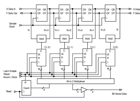
Figure 4: Functional diagram of the ASIC developed for the spectral-line correlator (the S21 system).

Figure 4 shows the organization of the ASIC. The $x$ and $y$ inputs are 3-level quantities, taking values $(1,0,-1)$. The shift registers are arranged so that $x$ and $y$ streams flow in opposite directions. Correlation function values are formed by connecting a multiplier-accumulator across each shift-register output. The multiplier output is biased, so that only positive products $(0,1,2)$, are formed, allowing accumulation in a simple up-counter. Accumulation begins with a 2-bit adder, whose output synchronously clocks a 23-bit ripple counter. Adder outputs are clocked into this counter at a fixed rate so that the mean value of the accumulator is constant even though the sample rate is adjusted when the overall bandwidth is changed. The system microprocessor detects overflows of the most significant accumulator bit, and extends the accumulation interval to 5.6 s.

The cross-correlation function is under-sampled in the ASIC because the delay interval is $2\tau$, where $\tau$ is the period of the sampling clock. By adding a second ASIC with one input delayed by $\tau$, the correlation function can be fully sampled. Alternatively, if the input signals are sampled at $2f_{N}$, a fully sampled correlation function is obtained (this is the normal mode of operation). For auto-correlation, a correlation function with one point at zero lag can be created by delaying one input by one half-lag.

5.3 408-MHz continuum correlator

The C74 correlator was designed to carry out interferometer signal-processing operations in simple software procedures to the maximum extent feasible (Lo et al. Lo84 (1984)). Figure 5 is a diagram of the system, showing the distribution of signal-processing functions between hardware and software.

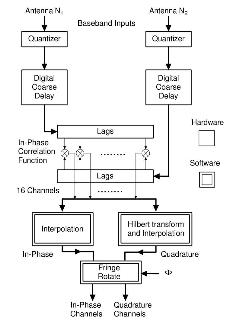
Figure 5: Functional diagram of the correlator used with the 408 MHz continuum channel of the telescope (the C74 system). The division of functions between hardware and software is indicated.

Incoming signals are sampled at 16 MHz and coarse delay is inserted in steps of one cycle of this clock (62.5 $\mu$s). A 16-point correlation function is generated. The in-phase visibility is retrieved from this function by interpolating to the exact geometrical delay. The quadrature visibility, which contains independent information, is also derived from this function. It is calculated by convolving the in-phase correlation function with the kernel function of a band-limited Hilbert transform. Since the in-phase and quadrature visibility outputs are required at only a single value of delay, the convolution degenerates to a simple dot product, requiring multiplication of each value of the correlation function by a matching coefficient from the kernel function. This is a simple and quick operation in the microprocessor (see Lo et al. Lo84 (1984) for details). A small error (of the order of 5%) arises in the derivation of the quadrature visibility because of truncation of the kernel. The error is mostly corrected by a multiplication factor. The residual error is much smaller than the decorrelation arising from bandwidth smearing.

Delay equalization is a continuous process, since the required path compensation is continuously changing as the Earth rotates. Precision of the compensation is high, limited only by the numerical precision of the interpolation arithmetic and the rate at which interpolation is performed. This confers an advantage over systems where delay is inserted in discrete steps. Such steps affect the phase of the correlator output, and must be corrected for, either before or after correlation.

5.4 Correlator linearity

Quantization of the baseband signals introduces non-linearities in the correlator output, which can lead to substantial artefacts in images (both H i-line and continuum) when bright Galactic objects lie in the field. Because of its sensitivity to extended structure, this telescope is more prone to this problem than other synthesis telescopes which resolve out most of the broad emission.

There are two approaches to the derivation of accurate visibilities using a digital correlator. In one approach, the signal level at the input to the A/D converter is held constant at the optimum level (see Figure 3). Under these circumstances, a 3-level correlator yields a value of correlation coefficient, $\rho$, linear within 1% up to values of $\rho=0.38$. However, to recover accurate visibility amplitudes requires accurate tracking of variations of system noise temperature. The alternative, which we have adopted, is to stabilize receiver gain through the system but to allow the signal level at the A/D converter input to vary (caused, for example, by variations of atmospheric emission and received ground radiation as a function of antenna elevation angle). This approach requires the development of algorithms to linearize correlator output. The algorithms convert the output of the correlators (separate algorithms have been developed for the 3-level and 14-level correlators) into an accurate measure of cross-power in the face of changes of system temperature of as much as 30%. The algorithms must be applicable to both auto- and cross-correlators, and must therefore be able to handle correlation coefficients as high as $\rho=1.0$. However, $\rho$ can also be high in the cross-correlator: when observing H i emission with the 12.86-m baseline, $\rho$ can rise to values as high as 0.7.

The algorithms proceed by first linearizing the autocorrelator response to derive an accurate measure of the variance of the input signal. Using this measurement, the cross-correlator response is linearized to obtain an accurate value of cross-power. The equations describing the correlator output in terms of its inputs cannot be directly inverted. Instead we use series approximations, following the ideas of Kulkarni & Heiles (Kulkarni80 (1980)) and D’Addario et al. (D'Addario84 (1984)). However, the correlator becomes increasingly non-linear as the input signal increases, spending a greater fraction of time above the highest quantizer decision level. The coefficients of the series inversion formula therefore must vary with input signal level. In our algorithm, these coefficients are themselves estimated by evaluating a series. Details of the linearization algorithms can be found in Hovey (Hovey98 (1998)). Their application reduces errors of as much as 30%, which occur in common observing conditions with this telescope, to less than 0.1%.

6 Software

The observing software comprises a combination of Unix-based tasks running on an IBM RS/6000, and a set of software tasks which run on Motorola-68000-based microprocessors (Figure 6). The RS/6000 system provides high-level synchronization, scheduling and data storage, while the true real-time work of data collection and sampling is done by the microprocessors. After data are collected, they are transferred via an ethernet connection to another IBM RS/6000 system, where the data are processed through automatic error-detection and flagging routines and inserted into a database awaiting final calibration and imaging, which is carried out once all the data required for a complete synthesis have been collected. (Twelve observations of 12 hours each are required to obtain all the data needed for imaging; see §8).

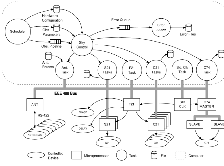
Figure 6: The telescope control software. C21, S21 and C74 are the three correlators described in section 5. F21 denotes the task and microprocessor which control the 1420 MHz receiver (frequency, phase, and delay). SID CLK is the sidereal clock. At the completion of an observation all files indicated are transferred via an ethernet connection to another computer where further processing occurs.

6.1 Telescope Control Software

The user interface to the observing system (Figure 6) is the program SCHEDULER, which allows the user to initiate observations of the program field and calibration observations, check on their progress, and abort them. A “template” consisting of a list of observations specified by field centre, duration, and starting time or hour angle may be entered, with individual sub-systems selectively chosen for each. SCHEDULER checks that the observations are possible within the antenna horizon limits, and the list is then placed in the observing queue.

Observing-system tasks communicate via serial polling over an IEEE 488 interface with microprocessors embedded in the various sub-systems of the telescope. These tasks read the sidereal clock, log messages generated by the observing system, and provide two-way communication with the microprocessors. Global synchronization between the sub-systems is performed by the program SKY_ CONTROL using Unix IPC messaging via addresses assigned to each task.

SKY_CONTROL also processes the observing queue. It determines which sub-systems are needed, initializes control files, and signals sub-system tasks accordingly. It also creates a binary file containing all of the parameters and hardware settings needed for the observation. This file subsequently follows the data through post-observation processing software as a record of the state of the system when the data were acquired. Sub-system-specific ASCII parameter files are also generated, which are read by the controlling tasks and used to send start-up commands to the microprocessors.

Once an observation has begun, SKY_CONTROL goes into a wait mode, looking for either the end of the run, or an “ABORT” signal from SCHEDULER. At the end of an observation SKY_CONTROL checks the observing queue, and initializes the next observation, continuing until the queue is empty.

Observing-system timing is controlled by the sidereal clock. Its attached microprocessor sends the time, once per second, to a shared memory area which can be accessed by other tasks. The time is also directly distributed to the individual microprocessors.

6.2 Error Logging

All Unix tasks report errors to a central program, LOGGER, via an IPC message queue. LOGGER runs continuously and writes all messages to a terminal and into an ASCII output file. Upon completion of an observation, the file is closed, tagged to the observation, and a new file is started. This tagged file follows the observation data into the post-observation processing area, and is used as input to the flagging programs for initial editing of bad data.

6.3 Post-Observation Processing

When an observation is complete, SKY_CONTROL moves the data across an ethernet link to an off-line post-observation processing area on disk, and spawns sub-shells to run command procedures. These are typically Unix shell scripts which call a sequence of FORTRAN-based programs that each perform a specific operation on the data. Important information and statistics may be generated by these programs, and are written to a processing log file, which the user checks in order to verify the health of the system and the validity of the data.

Since Synthesis Telescope observing projects are typically spread over several days, a number of project-specific databases are maintained, into which each newly processed observation or calibration is inserted. Each entry is indexed with the date of observation and the interferometer configuration. At any stage of data gathering these databases may be examined. However, aside from some manual flagging of bad data in each observation, the data are not generally further processed until all 12 observations for the project are complete.

Once all the data are available, an operator uses a graphics-based visibility editor to flag (but not remove) any remaining bad data. Appropriate calibration parameters for amplitude, phase, cross-polarization, and spectrometer passband-flattening, derived from calibration observations, are extracted from global databases and stored in a project-specific table. The data and accompanying tables are then processed to remove bad data and apply calibration. The resulting databases are suitable for gridding and Fourier transforming into images.

Images from the Synthesis Telescope are generally analyzed using an extensive suite of locally written software, designed to provide optimal results from Synthesis Telescope data, taking into account known instrumental effects. A detailed description of this suite of software is given in Higgs, Hoffmann & Willis (1996) and Willis (Willis99 (1999)).

7 Polarimetry

As described above, the C21 correlator measures cross-correlations of all combinations of polarizations; 1420-MHz continuum polarimetry became available on the Synthesis Telescope in 1993 (see Smegal et al. Smegal97 (1997)).

The antennas of the Synthesis Telescope are equatorially mounted, with feeds that cannot be rotated relative to the reflector, so the beam pattern always has a fixed orientation on the sky. While this has many advantages, it does complicate separation of spurious instrumental polarization from source polarization. Corrections for instrumental polarization must be determined by observing sources with little or no intrinsic polarization. The method by which these corrections are determined is discussed in detail by Smegal et al. (Smegal97 (1997)); put briefly, in the absence of an actual polarized signal, the cross-polarization correlations provide information about the orthogonality of the nominal LHCP and RHCP signals on each antenna, also known as “leakage”. The leakage terms measured for the Synthesis Telescope using 3C 147 and 3C 295 amount to between 1 and 5% on most antennas, although one antenna has about 10% leakage. If left uncorrected, these errors produce spurious instrumental polarization at the field centre amounting to several percent of the total flux. After correction, the residual instrumental polarization at the field centre is reduced by about an order of magnitude to 0.25% of the total intensity.

To measure polarization angle it is necessary to measure the phase difference between RHCP and LHCP channels on one antenna, an arbitrarily chosen reference. This is achieved by observing 3C 286, a strongly polarized, compact source with a fractional polarization of 9.25% and polarization angle of 33° at 1420 MHz. Polarimeter accuracy is 5° in polarization angle, and 10% in polarized intensity. The precision of the polarization angle measurements is also limited by ionospheric Faraday rotation, which amounts to about 3° in polarization angle between day and night (at present no correction is applied).

The off-axis polarization properties of the instrument are very good, and useful results can be obtained up to $90^{\prime}$ from the field centre. The residual instrumental terms rise approximately quadratically from the field centre, reaching about 10% of total flux at this radius. Empirical corrections, determined by observing 3C 147 and 3C 295 at various positions in the field and interpolating to intermediate positions, are applied to remove this increase. These corrections have been measured three times over a three-year period; they are very stable.

At present, deviations from circularity of the feeds are not accounted for. Since the data are processed as if the polarizations were purely circular, a small amount of any incident linear polarization is actually ascribed to circular polarization (Stokes $V$). This has little effect on linear polarimetry, but severely limits the ability of the telescope to detect and measure circular polarization. This has minimal impact on the astrophysical questions addressed by the telescope. For details see Smegal et al. (Smegal97 (1997)).

7.1 Rotation Measure

An important aspect of polarization studies is determining rotation measure to de-rotate observed polarization angles and recover the orientation of the intrinsic magnetic field. The sensitivity of the Synthesis Telescope to Faraday rotation is thus an important consideration. At 1420 MHz, a rotation measure of 4 rad m^-2 is required to produce a change in observed polarization angle of 10°, which is the limit of detectability with the present system.

In an image made from all 4 available bands, a rotation measure of approximately 330 rad m^-2 would cause 10% depolarization, with complete depolarization occurring for a rotation measure of $1.2\times 10^{3}$ rad m^-2. In a single band these figures are over 5 times higher, $1.7\times 10^{3}$ rad m^-2 and $6.6\times 10^{3}$ rad m^-2, respectively.

Since the 4 bands are available for separate processing, it is possible to use the frequency-dependent polarization angle to derive rotation measure. However, the relatively small span of frequency available imposes fairly high limits on the detectable rotation measures: 100 rad m^-2 is required to produce a change in angle of 10° between the centres of bands A and D (see Fig. 2).

8 Observing strategies

The east-west nature of the Synthesis Telescope requires that an object be tracked for 12 sidereal hours to obtain full hour-angle coverage. We describe this as an observation, although the total duration may sometimes be less than 12 hours. Twelve such observations produce a complete set of visibilities, fully sampling the available baselines; we describe such a set of data as an observation set.

In normal use the telescope is scheduled in a 4-day cycle, during which 7 back-to-back 12-hour observations with interleaved calibrations are completed, leaving approximately 8 hours per cycle for moving antennas and maintenance. The cycle is repeated 12 times to gather data on all possible spacings for the 7 fields. Occasional equipment failure and additional maintenance can add an extra day per field; an observing rate of 46 to 52 fields per year can be achieved in this mode of operation.

8.1 Calibration

Amplitude calibration and phase referencing are achieved by observing a set of strong, compact calibration sources which are known not to be time variable. The derivation of calibration coefficients uses standard antenna-based algorithms, with the complication that, since the Synthesis Telescope has a very wide field-of-view, it is necessary to account for nearby extraneous sources, which would otherwise cause undesirable hour-angle (and possibly time) dependencies. To this end, visibility models of the region surrounding each calibrator have been derived from observations, and are used to remove the effects of the extraneous sources. These models are updated periodically to allow for possible source variability, and are used routinely in deriving the calibration coefficients.

The most commonly used calibrators are listed in Table 5. The flux densities used for these sources are internally consistent and referenced to 3C 286. The flux densities adopted for the calibrators, based on measurements made in 1994, are consistent with the scale of Ott et al. (1994). The same sources are used to determine polarization calibration parameters. The stability of telescope gain and phase is such that it is only necessary to observe a calibrator prior to and following each 12-hour observation. Variations on shorter time-scales are corrected using self-calibration techniques.

Table 5: Calibration sources

Source	$S_{408}$ (Jy)	$S_{1420}$ (Jy)	$p_{1420}$ (%)	$\theta_{1420}$ (°)
3C 48	38.9	15.7	0.6	–
3C 147	48.0	22.0	$<0.25$	–
3C 286	not used	14.7	9.25	33.5
3C 295	54.0	22.1	$<0.25$	–
Note: quoted flux densities are based on measurements
made in 1994

Calibration of the spectrometer is difficult because the narrow channel bandwidth leads to high noise levels in individual channels. Calibration is achieved in a two-step process, by using calibration coefficients measured in the continuum bands. At the point where IF signals enter the central telescope building, a broadband noise signal can be injected into all IF paths, at a level sufficient to produce a correlation coefficient of $\sim 0.3$, adequate to give an accurate measurement of gain and phase in each spectrometer channel in 15 minutes. The continuum calibration measures antenna-based gain and phase which vary relatively slowly with frequency, but may vary with time. The IF calibration measures mostly the channel-to-channel amplitude and phase differences, which arise largely in the filters which define the bandpass, just before the signals are digitized; these are quite stable with time. This IF calibration is performed once every 4 days.

In later stages of image processing, amplitude and phase corrections are determined for individual antennas from self-calibration of Stokes $I$ images. These corrections are also applied to polarimeter images. Under some circumstances it is beneficial to apply them to H i images (e.g. when there is a strong continuum source in the field).

8.2 Antenna tracking and pointing

The antennas are capable of tracking down to an elevation of 12°, so the observable sky from the observatory’s terrestrial latitude of 49° nominally extends from declination $-29$° to +89°  (the latter imposed by the telescope drive system). However, full hour-angle coverage is possible only for declinations north of +18°. Sources north of declination +54° are circumpolar, and there is an overlap in hour-angle coverage at lower culmination, making it possible to track a circumpolar source for 26 sidereal hours without interruption. Non-sidereal tracking rates are available for observing solar-system objects.

Since they are equatorially mounted, the antennas track only in hour angle, although pointing corrections are made in both hour angle and declination. A pointing model for each antenna accounts for zero offset and ellipticity of the position encoders, misalignment of the polar axis, and non-orthogonality of the declination and hour-angle axes. These parameters are empirically determined from “nodding” observations of selected calibrators at many hour angles and declinations. A “nod” consists of measurements on-source and at 4 off-source positions situated 1° north, south, east, and west of the source, to which two-dimensional gaussians are fitted to obtain errors in hour angle and declination. The r.m.s. pointing accuracy across the observable sky is $2.4^{\prime}$ in R.A. and $3.1^{\prime}$ in Dec.

For a given observation, the pointing corrections at the declination of interest are calculated from the pointing model for every 30 minutes of hour angle, and interpolated linearly to intermediate hour angles. The tracking accuracy is then determined by a feedback loop in the control system, which measures the deviation of the antenna position from the requested position; at present errors in antenna position exceeding $3^{\prime}$ are corrected. Such corrections typically occur on timescales of 30 minutes.

9 Performance

9.1 Synthesized beams

The synthesized beam of the Synthesis Telescope depends on the taper applied in the u-v plane; details of synthesized beams are given in Table 6. A uniform weighting is always applied when making images from the telescope. The objectives of research with this telescope usually benefit more from better sensitivity and lower sidelobe levels than from high spatial resolution, so a Gaussian taper falling to 20% at $144L$ is typically applied to the u-v plane.

Table 6: Details of synthesized beams

Weighting	Frequency	Beamwidth	First sidelobe		Second sidelobe
	(MHz)	(half power)	level	radius	level	radius
Untapered	1420	$49^{\prime\prime}$	$-13$%	$1^{\prime}$	5.9%	$1.65^{\prime}$
Untapered	408	$2.8^{\prime}$	$-13$%	$3.5^{\prime}$	5.9%	$5.85^{\prime}$
Gaussian∗	1420	$58^{\prime\prime}$	$-2$%	$1^{\prime}$	2.4%	$1.65^{\prime}$
Gaussian∗	408	$3.4^{\prime}$	$-2$%	$3.5^{\prime}$	2.4%	$5.85^{\prime}$
∗ A Gaussian taper falling to 20% at $144L$ (617.1 m)

9.2 Field of view

The half-power beamwidth of the antennas is $107.2^{\prime}$ at 1420 MHz and $332.1^{\prime}$ at 408 MHz, but experience has shown that the usable field of view extends at least to the 10% level of the respective primary beams (diameters of $187^{\prime}$ and $578^{\prime}$, respectively). Empirical measurements show that these beams are well approximated by a function of the form $\cos^{6}(q_{\nu}r)$. If $r$ is the radius in degrees, $q_{1420}=30.24$, and $q_{408}=9.762$. Precise knowledge of the beam function is required for accurate mosaicing of images of individual fields.

9.3 Bandwidth and time-averaging effects

Wide-field imaging is an important aspect of the Synthesis Telescope, so off-axis effects must be carefully considered.

The continuum bands at 1420 MHz span 35 MHz, and, owing to differential delay effects, if the entire band were assumed to be at the nominal centre frequency there would be a reduction in point-source sensitivity of approximately 50% at a radius of $90^{\prime}$. This would be accompanied by a radial smearing of a point source to approximately twice the nominal beamwidth; while this preserves total flux, it is clearly unacceptable for high-fidelity imaging.

By treating the four 7.5 MHz continuum bands separately during imaging, taking into account the actual centre frequency of each, the reduction in point source sensitivity at $90^{\prime}$ is only 5%, with a comparable amount of source distortion (see Bridle & Schwab (1989)). The 3.5-MHz bandwidth at 408 MHz reduces the point-source sensitivity by about 10% at a radius of $300^{\prime}$, again with a similar amount of source distortion.

Effects due to time averaging are also a factor. At the radii of $90^{\prime}$ at 1420 MHz and $300^{\prime}$ at 408 MHz, the visibility averaging period of 90 s reduces point-source sensitivity by about 8% in a 12-hour observation, with source distortion of similar magnitude in the azimuthal direction. The combined effect of bandwidth and time-averaging smearing is then a worst-case reduction of point-source sensitivity of about 13% at 1420 MHz and 17% at 408 MHz, with both radial and azimuthal distortions. Software written for analyzing Synthesis Telescope images takes these effects into account when determining, for example, point-source fluxes.

9.4 Noise in Images

The r.m.s. noise, $\Delta S$ (W m^-2 Hz^-1), in an image made by a synthesis telescope is (Crane & Napier (1989))

$$\Delta S={{W\sqrt{2}kT_{S}}\over{\eta_{c}\eta_{A}A\sqrt{N_{b}N_{\rm IF}{\Delta f}\tau}}}$$

where $W$ is a factor that depends on the weighting scheme applied to the visibilities during imaging, $k$ is Boltzmann’s constant, $T_{S}$ is the system temperature (K), $\eta_{c}$ is the correlator efficiency (defined in §5), $\eta_{A}$ is the aperture efficiency of the antennas, each with area $A$ (m²), $N_{b}$ is the number of baselines, $N_{\rm IF}$ is the number of IF channels, each of bandwidth $\Delta f$ (Hz), and $\tau$ is the integration time (s). $N_{\rm IF}=1$ for a single polarization, and $N_{\rm IF}=2$ when two polarizations are received.

The brightness-temperature sensitivity in K is

$$\Delta T={{1}\over{\Omega}}{{\Delta S\lambda^{2}}\over{2k}}$$

where $\Omega$ is the synthesized beam area and $\lambda$ is the wavelength.

The factor $W$ is unity for a naturally weighted image, but this weighting scheme is never used with this telescope. Two weighting schemes used are (a) uniform weighting, for which $W=2$, and (b) Gaussian tapering of uniformly weighted data, tapering to 20% at the longest spacing, for which $W=1.33$. The brightness temperature sensitivity is $\Delta T=0.25\Delta S\sin\delta$ K for case (a) and $\Delta T=0.18\Delta S\sin\delta$ K for case (b).

Table 7 shows the calculated sensitivities for each of the three telescope outputs, and compares these predictions with measured noise levels from images. At 408 MHz the thermal noise limit is not reached because of confusion.

Table 7: Telescope sensitivity

	1420 MHz	1420 MHz	408 MHz
	continuum	spectrometer	continuum
$T_{S}$, K	60	60	150∗
$\eta_{A}$	0.55	0.55	0.60
$\eta_{c}$	0.985	0.88	0.88
$N_{b}$	21	12	21
$N_{IF}$	2	2	1
$\Delta f$, MHz	30	$B/160^{\dagger}$	3.5
$W$	2.0	1.33	2.0
$\Delta S_{theor}$ mJy/beam	0.28	$20B^{-0.5}$	3.0
$\Delta T_{theor}$ K	$0.071\sin\delta$	$3.5B^{-0.5}\sin\delta$	$0.75\sin\delta$
$\Delta S_{meas}$ mJy/beam	0.27	$18B^{-0.5}$	3.8
∗ Includes $T_{sky}=45$ K, a typical value in the Galactic plane
† $B$ is the overall spectrometer bandwidth in MHz

The dynamic range achieved with the telescope varies with frequency and region observed. In the 1420 MHz continuum channel, dynamic ranges of $10^{4}$ are commonly achieved. The limits to this performance are, at the low end, system noise, and, at the high end, artefacts in the vicinity of strong sources. Artefacts, which are very difficult to remove by normal processing, rise above the thermal noise limit when telescope pointing is closer than 3° to Cas A or Cyg A. At 408 MHz, the dynamic range achieved is about $5\times 10^{3}$, for offsets greater than 5° from strong sources.

9.5 Imaging Performance

Owing to the thorough sampling of baselines in a $12\times 12$ hour observation set, the images produced by the Synthesis Telescope have very low sidelobe levels and excellent sensitivity to extended structure. This can be seen clearly in Figure 7, which shows part of the data from one 1420-MHz field from the Canadian Galactic Plane Survey. The extended object which dominates Stokes $I$ images of this field is the H ii region W5 (IC 1848), in the Perseus arm of the Galaxy at a distance of $\sim 2$ kpc. The “raw” image (top left), is made from the calibrated visibilities after editing interference, but before application of any image processing routines. The large emission regions are surrounded by depressions, produced by the lack of data for baselines $<3L$. The final image, after incorporation of single-antenna data, is shown at upper right.

The raw Stokes $U$ image (lower left) shows structure on many scales, totally unrelated to that seen in the $I$ image. These polarization structures arise from Faraday rotation along the line of sight – they are not intrinsic features of the emission source. The large elliptical polarization structure is discussed briefly in §10.

The lower right panel shows one of the 256 spectral-line channels; the data have been edited and a continuum image, formed from spectrometer channels free of H i emission, has been subtracted, but no single-antenna data have been added.

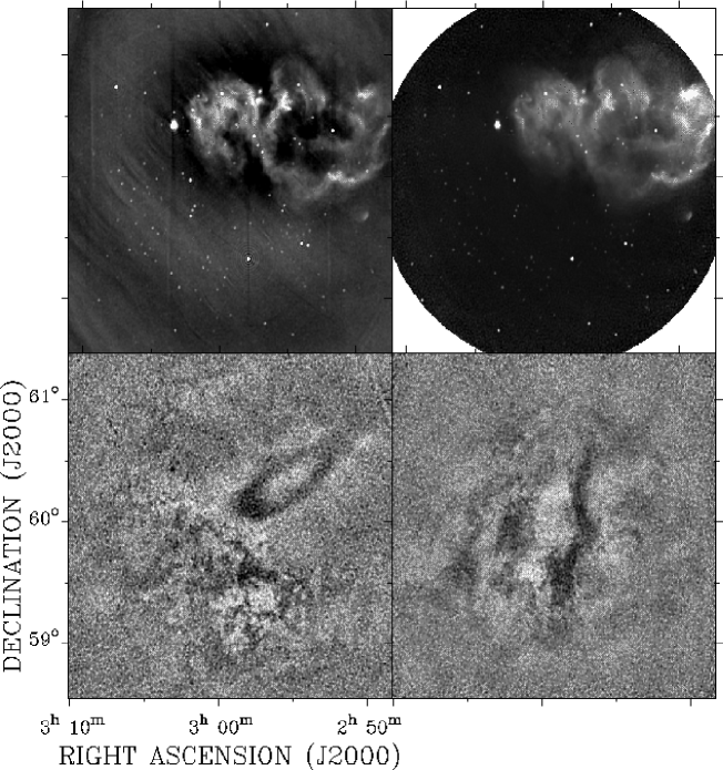
Figure 7: Images at 1420 MHz of a field containing the H ii region W5. Top left: continuum image made from calibrated visibilities after editing interference, but before application of any image processing routines. Top right: fully processed image with single-antenna data incorporated. A correction has been applied to compensate for the primary beam of the antennas. The circular boundary is at a radius of $90^{\prime}$. Lower left: image in Stokes parameter $U$. Other than editing of interference, no processing has been applied. Lower right: H i image in one of 256 channels of the spectrometer. Continuum emission has been estimated from end-channels of the spectrometer and subtracted. No single-antenna data have been added to either of the lower two images.

10 Astronomical applications

We have described a synthesis telescope uniquely suited to observation of the Galactic ISM. While its resolution ($\sim 1^{\prime}$) is modest compared to some synthesis telescopes (e.g. the VLA), its sensitivity to extended structure is superior, and it offers significantly different performance from single-antenna telescopes. In this section we discuss a few examples of results obtained with the telescope, chosen to illustrate its unique capabilities. A more detailed discussion will be found in Taylor et al. (2000).

At distances of 2 to 10 kpc, the $1^{\prime}$ angular resolution of the telescope translates into a physical resolution of 0.6 to 3 pc, which has proved to be a good match to significant ISM structures. The interstellar H i shows extensive filamentary structure on these scales both within the Galactic plane (Normandeau et al. (1997)) and at high latitudes (Joncas et al. (1992)). While the origin of the fine structure in this emission is not completely understood, it seems very often to be related to interfaces between the atomic phase and some other constituent of the ISM, or to energy injection, as from stellar winds.

Experience with the telescope has shown that there are significant ISM phenomena which extend over many degrees, but require arcminute angular resolution for their detection. An example is provided by the discovery of a Galactic chimney by Normandeau et al. (1996). This structure is a conduit for radiation and material from the disk to the halo, and it is outlined by a sharp interface between the H i exterior and the ionized interior. Its size is $\sim 5$°, equivalent to several hundred pc at the distance of the Perseus Arm ($\sim 2$ kpc) . It is nevertheless extremely difficult to detect in the survey data of Hartmann & Burton (1997): even though that survey has much higher nominal sensitivity than the Synthesis Telescope, its angular resolution is only $36^{\prime}$.

Similar considerations apply to the detection of thermal and non-thermal continuum objects. The continuum sensitivity of the telescope (listed in Table 7) translates into sensitivity to thermal emission measure (at both frequencies) of $\sim 27$ cm^-6 pc and sensitivity to synchrotron emission of $\sim 4\times 10^{-23}$ W m^-2 Hz^-1 sr^-1, also at both frequencies. An example is provided by the detection of large supernova remnants (SNRs) of low surface brightness. For example, Landecker et al. (1990) discovered the SNR G65.1+0.6, whose size is $90^{\prime}\times 51^{\prime}$. The overall surface brightness of this object is about half of the nominal rms sensitivity quoted above, indicating the importance of filamentary structure in making such objects detectable.

Polarization imaging at 1420 MHz allows detailed analyses of discrete emitters of polarized radiation, particularly SNRs. For example, Leahy et al. (1997) have mapped the polarized emission from the full extent of the Cygnus Loop. However, only part of the SNR is strongly polarized, with some of the shell emission depolarized by strong Faraday rotation within a thermal electron component mixed in with the compressed fields and synchrotron emitting particles.

While SNRs are prominent objects in Stokes $I$ images, most are barely significant in images of Stokes $Q$ or $U$. The dominant feature in all polarization images made close to the Galactic Plane is widespread, low-level structure, seen most prominently in polarization angle. This structure is understood as the result of Faraday rotation in the magnetized ISM acting on polarized signals from the diffuse Galactic synchrotron radiation. It tells us less about the emitter than it does about the medium through which the polarized radiation has travelled.

The study of this phenomenon is providing a new window on the ISM, through its sensitivity to magnetic fields and low-density ionized material. The frequency of 1420 MHz seems ideal for such studies near the Galactic plane, where the properties of the Faraday screen lead to a change in polarization angle that is neither too small to produce measurable changes nor so large that it causes depolarization within the beam or the bandwidth of the telescope. The large elliptical feature seen in Figure 7 (lower left panel), for example, which is very uniform in structure in contrast to its chaotic surroundings, is understood as just such a manifestation of ionized material in the inter-arm region (Gray et al. (1998)). Other polarization results (Gray et al. (1999)) have led to the detection of an extended envelope of a large H ii region, and the measurement of the magnetic field in that envelope. In both cases, the H ii regions themselves produce depolarization due to the turbulent, high-density ionized material within them.

References

- (1) Anderson, M.D., Landecker, T.L., Routledge, D., Vaneldik, J.F., 1991, Radio Science, 26, 353
- (2) Bowers, F.K., Klingler, R.J., 1974, A&AS, 15, 373
- Bridle & Schwab (1989) Bridle, A.H., & Schwab, F.R., 1989, in R.A. Perley, F.R. Schwab, F.R., A.H. Bridle, eds, Synthesis Imaging in Radio Astronomy, ASP Conference Series v.6, 247, Astronomical Society of the Pacific, San Francisco.
- (4) Burke, I.E., Tapping, K.F., 1995, Solar Phys., 157, 295
- Costain et al. (1976) Costain, C.H., Higgs, L.A., MacLeod, J.M., Roger, R.S., 1976, AJ, 81,1
- Crane & Napier (1989) Crane, P.C., Napier, P.J., 1989, in Synthesis Imaging in Radio Astronomy, R.A. Perley, F.R. Schwab, A.H. Bridle (eds), ASP Conference Series v.6, 139, Astronomical Society of the Pacific, San Francisco.
- (7) D’Addario, L.R., Thompson, A.R., Schwab, F.R., Granlund, J., 1984, Radio Science, 19, 931
- Faison et al. (1999) Faison, M.D., Goss, W.M., Goss, P.J., Taylor, G.B., 1999, in New Perspectives on the Interstellar Medium, A.R. Taylor, T.L. Landecker, G. Joncas (eds), ASP Conference Series v.168, 379, Astronomical Society of the Pacific, San Francisco.
- (9) Granlund, J., Thompson, A.R., Clark, B.G., 1978, Trans. IEEE, EMC-20, 451
- Gray et al. (1998) Gray, A.D., Landecker, T.L., Dewdney, P.E., Taylor, A.R., 1998, Nature, 393, 660
- Gray et al. (1999) Gray, A.D., Landecker, T.L., Dewdney, P.E., Taylor, A.R., Willis, A.G., Normandeau, M., 1999, ApJ, 514, 221
- Hartmann & Burton (1997) Hartmann, D., Burton, W.B., 1997, Atlas of Galactic Neutral Hydrogen, Cambridge University Press, Cambridge
- Haslam et al. (1982) Haslam, C.G.T., Salter, C.J., Stoffel, H., Wilson, W.E., 1982, A&AS, 47, 1
- Higgs, Hoffmann & Willis (1996) Higgs, L.A., Hoffmann, A.P., Willis, A.G., 1996, in Astronomical Data Analysis Software and Systems VI, G. Hunt, H.E. Payne (eds), ASP Conference Series v.125, Astronomical Society of the Pacific, San Francisco.
- (15) Hovey, G.J., 1998, Thesis, University of British Columbia, Vancouver
- Joncas et al. (1992) Joncas, G., Boulanger, F., Dewdney, P.E., 1992, ApJ, 397, 165
- (17) Kallas, E., Reich, W., 1980, A&AS, 42, 227
- Karpa (1989) Karpa, D.R., 1989, Thesis, University of Alberta, Edmonton
- (19) Klingler, R.J., 1974, Thesis, University of British Columbia, Vancouver
- (20) Kulkarni, S.R., Heiles, C., 1980, AJ, 85, 1413
- (21) Landecker, T.L., 1984, Trans. IEEE, IM-33, 78
- (22) Landecker, T.L., Anderson, M.D., Routledge, D., Smegal, R.J, Trikha, P., Vaneldik, J.F., 1991, Radio Science, 26, 363
- Landecker et al. (1990) Landecker, T.L., Clutton-Brock, M., Purton, C.R., 1990, A&A, 232, 207
- (24) Landecker, T.L., Vaneldik, J.F., 1982, Trans. IEEE, IM-31, 185
- Leahy et al. (1997) Leahy, D.A., Roger, R.S., Ballantyne, D., 1997, AJ, 114, 2081
- (26) Lo, W.F., Dewdney, P.E., Landecker, T.L., Routledge, D., Vaneldik, J.F., 1984, Radio Science, 19, 1413
- Normandeau et al. (1996) Normandeau, M., Taylor, A.R., Dewdney, P.E., 1996, Nature, 380, 687
- Normandeau et al. (1997) Normandeau, M., Taylor, A.R., Dewdney, P.E., 1997, ApJS, 108, 279
- Ott et al. (1994) Ott, M., Witzel, A., Quirrenbach, A., Krichbaum, T.P., Standke, K.J., Schalinski, C.J., Hummel, C.A., 1994, A&A, 284, 331
- (30) Reich, P., Reich, W., 1986, A&AS, 63, 205
- (31) Reich, P., Reich, W., Fürst, E., 1997, A&AS, 126, 413
- (32) Reich, W., 1982, A&AS, 48, 219
- (33) Reich, W., Reich, P., Fürst, E., 1990, A&AS, 83, 539
- Roger & Costain (1976) Roger, R.S., Costain, C.H., 1976, A&A, 51, 151
- (35) Roger, R.S., Costain, C.H. , Lacey, J.D., Landecker, T.L., Bowers, F.K., 1973, Proc. IEEE, 61, 1270
- (36) Scheffer, H., 1975, Europ. Microwave Conf., Hamburg
- Simmons (1952) Simmons, A.J., 1952, Proc. IRE, 40, 1089
- (38) Smegal, R.J., Landecker, T.L., Vaneldik, J.F., Routledge, D., Dewdney, P.E., 1997, Radio Science, 32, 643
- Taylor et al. (2000) Taylor, A.R., Landecker, T.L., Dewdney, P.E., Martin, P.G., 2000, AJ, submitted
- (40) Thompson, A.R., Moran, J.M., Swenson, G.W., 1986, Interferometry and Synthesis in Radio Astronomy, John Wiley Sons Inc., New York
- (41) Trikha, P.K., Landecker, T.L., Routledge, D., Vaneldik, J.F., 1991, Electron. Lett., 27, 1682
- (42) Veidt, B.G., Landecker, T.L., Vaneldik, J.F., Dewdney, P.E., Routledge, D., 1985, Radio Science, 20, 1118
- (43) Walker, G., Vaneldik, J.F., Routledge, D, Landecker, T.L., Galt, J.A., 1988, Can. Elec. Eng. J., 13, 3
- (44) Weinreb, S., Fenstermacher, D.L., Harris, R.W., 1982, Trans. IEEE, MTT-30, 849
- (45) Willis, A.G., 1999, A&AS, 136, 603