Exploring Halo Substructure with Giant Stars: I. Survey Description and Calibration of the Photometric Search Technique

Abstract

We have begun a survey of the structure of the Milky Way halo, as well as the halos of other Local Group galaxies, as traced by their constituent giant stars. These giant stars are identified via large area, CCD photometric campaigns. Here we present the basis for our photometric search method, which relies on the gravity sensitivity of the Mg I triplet + MgH features near 5150 Å in F-K stars, and which is sensed by the flux in the intermediate band $DDO51$ filter. Our technique is a simplified variant of the combined Washington/DDO51 four filter technique described by Geisler [1984, PASP, 96, 723], which we modify for the specific purpose of efficiently identifying distant giant stars for follow-up spectroscopic study: We show here that for most stars the Washington $T_{1}-T_{2}$ color is correlated monotonically with the Washington $M-T_{2}$ color with relatively low scatter; for the purposes of our survey, this correlation obviates the need to image in the $T_{1}$ filter, as originally proposed by Geisler.

To calibrate our ($M-T_{2}$, $M-DDO51$) diagram as a means to discriminate field giant stars from nearby dwarfs, we utilize new photometry of the main sequences of the open clusters NGC 3680 and NGC 2477 and the red giant branches of the clusters NGC 3680, Melotte 66 and $\omega$ Centauri, supplemented with data on field stars, globular clusters and open clusters by Doug Geisler and collaborators. By combining the data on stars from different clusters, and by taking advantage of the wide abundance spread within $\omega$ Centauri, we verify the primary dependence of the $M-DDO51$ color on luminosity, and demonstrate the secondary sensitivity to metallicity among giant stars. Our empirical results are found to be generally consistent with those from analysis of synthetic spectra by Paltoglou & Bell [1994, MNRAS, 268, 793].

Finally, we provide conversion formulae from the ($M$, $M-T_{2}$) system to the ($V$, $V-I$) system, corresponding reddening laws, as well as empirical red giant branch curves from $\omega$ Centauri stars for use in deriving photometric parallaxes for giant stars of various metallicities (but equivalent ages) to those of $\omega$ Centauri giants.

1 Introduction

1.1 Survey Goals

Understanding the nature of the Milky Way halo – its shape, extent, density distribution, kinematics, abundance distribution and origin – has long been a central topic in astronomy. The importance of this endeavor has increased substantially with the growing, pervasive connections to a number of other astronomical enterprises bearing on such wide ranging astrophysical problems as, for example, the magnitude and distribution of dark matter and the frequency of microlensing events, the origin of the second parameter problem of horizontal branch morphology in globular clusters, the nature of high velocity HI clouds, the interaction of galaxies with their environment, and, of course, the origin and evolution of the Milky Way. In spite of the pressing need for a detailed picture of the halo, at present we still have only the most rudimentary prescriptions of, for example, the phase space distribution of halo stars. Unfortunately, for many applications we no longer can be satisfied with elementary analytical models of the halo. Indeed, the very suitability of such simple descriptions may now be questioned.

A number of new lines of evidence indicate that the halo of the Milky Way has not achieved a dynamically relaxed state. Confirmation of this rather old idea is a long time in coming. Studies of candidate “moving groups” of metal-poor stars with halo kinematics in the solar neighborhood were made long ago by Eggen and collaborators (Eggen & Sandage, 1959; Eggen, 1960), and the idea of a halo with significant structure in the form of intermingling “tube-like swarms” was a viable theoretical description at least 35 years ago (Oort, 1965). However, apart from consistent attention to the subject of halo “moving groups” by Eggen (1960; 1977; 1978; 1996, and references therein), until recently the subject of halo substructure has received little other interest, in deference to more prosaic descriptions of the Galactic halo – those easily described by relatively simple analytical prescriptions. This state of affairs was influenced perhaps, in part, by a growing emphasis on computer models of Galactic structure that relied on analytical density laws (Bahcall & Soneira, 1981; Robin & Crézé, 1986, et seq.), coupled with the lack of systematic observational efforts toward uncovering even first order global laws (e.g., density relations, amount of flattening, kinematical and chemical trends with position) along more than a small number of lines of sight, let alone deviations from these simple global descriptions. Moreover, the rather smoother phase space distributions of the “flattened halo” and Intermediate Population II (which may or may not be parts of one continuous population; see Majewski 1993, 1995), locally dominate the more extended halo component – what Oort (1965) refers to as the “pure races of the halo population II”. Indeed, that these flattened Galactic populations contain stars with chemodynamical properties (“high velocity” and low metallicity) that are typically considered “halo-like” has long vexed understanding of the true “mixture ratios” and individual chemodynamical properties of the various overlapping stellar populations (see, for example Nemec & Nemec, 1993). The more relaxed dynamical state of the locally more dominant, flattened metal-poor components of the Galaxy may have long distracted attention from an unrelaxed halo population filled with substructure.

With the latter point as preface, it is worthwhile, therefore, to clarify our own working conception of the “halo” – that Galactic component we aim to explore in the present survey – since the very definition of “halo” has taken on such a diversity of connotations. Presently fashionable “dual halo” models of the Milky Way – those containing both flattened, prograde rotating and spherical, slow to non- (or even retrograde) rotating metal-poor components (Hartwick, 1987; Majewski, 1993; Norris, 1994; Carney et al., 1996) – bear a resemblance to the commonly accepted Galactic descriptions at the 1957 Vatican Conference (O’Connell, 1958), when one appreciates that the properties of the Intermediate Population II (IPII) discussed there parallel properties assigned to the “new” flattened, contracted halo/thick disk components in today’s models. In the present survey, we are concerned with Oort’s “pure race” of Population II: the extended, more or less spherical distribution of stars with the most extreme kinematics in the Galaxy, where growing theoretical and observational work suggests evidence of past Galactic accretion events may be fossilized. The Intermediate Population II, “low” or “flattened” halo – which may all be the same thing (Majewski, 1994) – we address more fully in our parallel astrometric survey (e.g., Majewski, 1992; Crane & Majewski, 2000, et seq.).

In the last decade or so, a number of developments have spawned intense interest in the interaction of Milky Way-like galaxies with each other and with their satellites and clusters: e.g., (1) the popularity of Cold Dark Matter models of the universe, with the concomitant “bottom up” growth of structure from the collection of smaller subunits (e.g., Frenk et al., 1988), (2) the realization of the prevalence of gravitationally interacting galactic systems in the nearby universe (demonstrated of course by Arp 1966; and explored more recently by, for example, Mihos & Bothun 1997) and at high redshifts by van den Bergh et al. (1996), (3) the discovery of the formation of globular clusters (Ashman & Zepf, 1992; Schweizer et al., 1996) and dwarf satellites (Mirabel, Dottori & Lutz, 1992; Hunsberger, Charlton & Zaritsky, 1996) in the course of such gravitational interactions, (4) the discovery of new Galactic satellites (Cannon, Hawarden & Tritton, 1977; Irwin et al., 1990; Ibata, Gilmore & Irwin, 1995), possibly associated Galactic neighbors (van de Rydt, Demers & Kunkel, 1991), and distant globular clusters (e.g., Madore & Arp, 1982; Irwin, Demers & Kunkel, 1995) and the fact that some of these systems have complex star formation histories (e.g., Smecker-Hane et al., 1994; Grebel, 1997), and (5) the recognition of the complexities of the dynamics of the Local Group and the implications for the size of galactic dark matter components and the cosmological density, $\Omega$ (Zaritsky et al., 1989; Valtonen et al., 1993; Governato et al., 1997). New computer studies of galaxy interactions (McGlynn 1990; Moore & Davis 1994; Johnston, Hernquist & Bolte 1996; Kroupa 1997; Klessen & Kroupa 1998, but all predated by Toomre & Toomre 1972) confirm long-held notions (Oort 1965; see also the related results of Innanen & House 1970) that satellite galaxies, when experiencing tidal disruption by a larger galactic potential, can leave behind long-lived structures – Oort’s “tube-like swarms” – along the satellite orbit. The idea that these satellites themselves may not be dynamically relaxed systems (Kuhn & Miller, 1989; Burkert, 1997; Kroupa, 1997; Klessen & Kroupa, 1998; Johnston et al., 1999) has also played an important role in the debate on the existence of substantial dark matter halos in these systems (cf. discussion in Majewski et al., 2000, hereafter Paper II).

Hints of substructure in the Galactic halo that may be the “swarms” that are the hallmark of accretion of smaller stellar systems have been suggested in several surveys of halo stars undertaken since the concentrated effort of Eggen to find halo (and other) “moving groups” among stars in the solar neighborhood. This more recent evidence has most often been found in surveys of the more distant, “pure” halo, and most typically as clusterings of stars in distance and radial velocity – e.g., the clumps of distant blue horizontal branch stars in Sommer-Larsen & Christensen (1987), Doinidas & Beers (1989), and Arnold & Gilmore (1992). One very notable radial velocity-distance clump in the survey of distant stars by Ibata et al. (1995) is now recognized as the structural paradigm of the type of tidal events sought here – an extremely elongated, tidal structure forming through the destruction of the Sagittarius dwarf galaxy. Indeed, the Sgr galaxy was first identified through the clustering of radial velocities in distant giant stars, a technique we intend to exploit in the present survey.

Earlier evidence for possible tidal debris recognized as families of associated outer halo clusters and dwarf spheroidals was discussed by Kunkel & Demers (1976), Kunkel (1979) and Lynden-Bell (1982), and has received an increase in interest more recently (Majewski, 1994; Fusi Pecci et al., 1995; Lynden-Bell & Lynden-Bell, 1995; Palma, Majewski & Johnston, 2000). One “family” of clusters (including Arp 2, Terzan 7 and 8, M54, and Pal 12) is apparently associated with the paradigm tidal event, Sagittarius (Ibata et al., 1995; Dinescu et al., 2000). Phase space clumpings of more nearby, dwarf stars have also been identified by Rodgers, Harding & Walker (1990), Côté et al. (1993), Majewski, Munn & Hawley (1994a; 1996), and Helmi et al. (1999), with the clumps in the latter three works – delineated in all three dimensions of motion – very clearly being identified as halo members on the basis of both kinematics and abundance. A surprising implication of Majewski et al. (1996) is that the more distant halo appears to be dominated by phase space structure – i.e., very little “random”, dynamically relaxed halo field population exists outside of the IPII. This empirical result would appear to echo theoretical suggestions that a large fraction of the halo might contain substructure (Tremaine, 1993; Johnston, 1998).

Detailed surveys of the halo including both precision proper motions and radial velocities, like the Majewski et al. (1996) analysis, may be needed to understand the full spectrum of structure in halo phase space, and that particular survey continues to pursue that question. However, to cover any significant amount of area in this detailed manner presents a formidable and improbable task at present. Moreover, to carry out this kind of work to distances as large as those of the present retinue of Galactic satellites – possibly major contributors to the overall halo field star population – will need to await new generations of microarcsecond astrometry instruments, such as the Space Interferometry Mission. In the meantime, questions regarding the existence of halo substructure, its extent, filling factor, size spectrum, etc. may be approached even when full kinematical data may not be obtainable. The survey we describe here is aimed at divining and defining physical substructure in the halo when that substructure is coherent and has reasonable contrast above any well-mixed background in the occupied volume. A primary aim of the present survey is to probe to large Galactic distances with ease, and so provide a complement to the more detailed, but more confined, Majewski et al. (1996) proper motion-radial velocity survey of the halo and IPII. The greater distances probed in the giant survey described here lend certain advantages over a survey of more nearby stars, even one replete with full, 3-D kinematical information. While perhaps decreasing sensitivity to subtle, more diffuse, structures requiring a full analysis of phase space, exploring at great distances from the Galactic midplane unfetters the data and analysis from contamination by stars in the same survey volume having similar chemodynamical properties to, but coming from stellar populations (e.g., IPII, or the “lower halo”) other than, the “pure” halo. From the standpoint of uncovering detailed information on the history of the Galaxy from phase space substructure, surveys of distant halo stars also have the added benefit that remote tidal structures are longer lived in the softer gradient of the Galactic potential at large radii. Debris closer to the Galactic center becomes phase-mixed rather quickly, and loses spatial coherence that would otherwise be easily identifiable (although velocity coherence is increased – Helmi & White 1999). Distance also increases the contrast of strongly coherent structures against the background, because the linear width of a given structure subtends a smaller area on the sky, and the magnitude spread in the color-magnitude diagram from depth effects is decreased (see Majewski 1999), and because any smooth background of stars should have a rather steep density fall-off with Galactocentric radius (going as, say, $r^{-3}$).

1.2 Survey Approach

Recent work by Johnston et al. (1996) and Johnston (1998) makes it evident that kinematic substructure in the halo would be difficult to see with simple starcounting techniques. The densities of “star swarms” from dissociated Galactic satellites are simply too low to be detectable above the foreground curtain of disk and IPII dwarfs – a problem especially confounded when the swarms are at distances where the much smaller volume density of their luminous, evolved stars is the only signal likely to be observable. To make tidal streams in the outer halo more evident, it clearly would be beneficial to be able to reduce, or completely filter out, foreground disk contamination, to which main sequence stars make the greatest contribution redward of the field main sequence turnoff. The signal-to-noise of a systematic search could be increased substantially if one were able a priori to key on stars of a set absolute luminosity because then disk and IPII stars with this luminosity would be easily differentiated from outer halo stars simply by their substantially brighter apparent magnitudes. For example, halo RR Lyrae stars and horizontal branch stars, which have a relatively limited range of absolute magnitudes, are rather easy to identify on the basis of variability or color and have been used as tracers of halo structure (e.g., Saha, 1985; Kinman, Suntzeff & Kraft, 1994). On the other hand, horizontal branch stars are sufficiently rare that, while they can point to the presence of halo substructure, they may not be able to trace subtle or more tenuous halo substructure convincingly and/or thoroughly, as the rather small, candidate “moving groups” found by Sommer-Larsen & Christensen (1987), Arnold & Gilmore (1992), and Doinidas & Beers (1989) would suggest. Unevolved, main sequence stars would, of course, make up the bulk of any stellar stream, but it is too difficult at present to explore dwarf stars to very great distances over large areas, though this technique has been used to study deep, pencil beam surveys with large telescopes in small numbers of strategically placed directions (see, e.g., Gould et al., 1992; Reid et al., 1996).

For exploring halo substructure, giant stars may provide a reasonable compromise between the problems associated with the readily identifiable, but less numerous horizontal branch stars and the more common, but intrinsically faint dwarf stars. Giant stars are generally a few times more populous than horizontal branch stars in a given stellar population and provide the distinct advantage that they are bright enough to be imaged to great distances even with small telescopes. With giant stars large volumes of the outer Galaxy may be explored efficiently with small telescopes (where larger blocks of observing time are easier to come by) if a reasonable means can be found by which to pick out the giants from the foreground dwarfs.

There have been several K giant studies at high Galactic latitude (Yoss, Neese & Hartkopf, 1987; Ratnatunga & Freeman, 1985, 1989; Flynn & Freeman, 1993; Morrison, 1993) from which we can infer expected densities of Population II giants. Flynn & Freeman (1993) found $\sim$ 1 giant deg^-2 in a survey complete for the magnitude range $9.5\lesssim{V}\lesssim{11.0}$ covering $\sim 140$ deg² at the SGP. In several high Galactic latitude fields covering a total area of $60$ deg², Ratnatunga & Freeman (1985) found a mean density for Population II giants of order 2 deg^-2 in the magnitude range $13\lesssim{V}\lesssim{16}$. With an expected mean radial fall-off of the halo with Galactocentric radius as $\sim R_{GC}^{-3}$ we obtain a flat differential count of giants with magnitude (Paper II) and we may extrapolate that to $V\sim 21$ (distances of $\gtrsim 250$ kpc, for typical $M_{V}\sim-1$ halo metallicity giants) we should expect approximate mean densities of halo giants of $\lesssim 10$ deg^-2. Thus, it is clear that a survey for giant stars must cover large areas of the sky in order to garner reasonably large statistical samples. The requirement for large sky coverage drives the criteria to make our survey as efficient as possible at identifying giant stars.

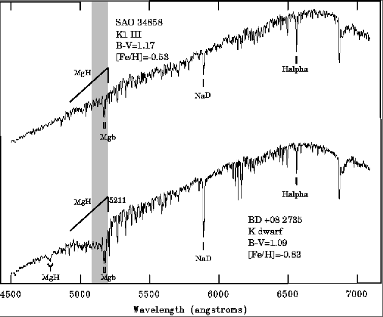
Figure 1: Comparison of spectra for K giant and dwarf stars of similar color and abundance, illustrating the dependence of the MgH + Mgb triplet on luminosity class. The location of the $DDO51$ filter bandpass is indicated by the shaded region. Note also the gravity-sensitivity of the MgH band near 4850 Å as well as the NaD doublet (Tripicchio et al., 1997).

It has long been known that the strength of the MgH + Mgb triplet feature at 5100 Å is strongly dependent on surface gravity (see Figure 1; Ohman, 1934; Thackeray, 1939), and it is a common technique to identify giants by their weak absorption in this part of the spectrum (Friel, 1987; Ibata & Irwin, 1997). Ratnatunga & Freeman (1983; 1985) showed that discrimination of K giants and dwarfs by this feature was possible with low resolution (20 Å ) objective prism plates from Schmidt telescopes, while McClure (1976) and Clark & McClure (1979) had already devised a technique by which to identify giants photometrically with a pair of intermediate band filters, centered at 4880 Å ($DDO48$ – “continuum”) and 5150 Å ($DDO51$ – “Mg”). This filter system has been applied to the giant surveys of Yoss & Hartkopf (1979); Hartkopf & Yoss (1982); Yoss, Neese & Hartkopf (1987).

Later, Geisler (1984, et seq.) showed that good photometric luminosity classification was still possible with the $DDO51$ filter (see Figure 1) when the continuum was measured with an appropriate broad band filter, in this case the $M$ filter of the Washington system (Canterna, 1976; Harris & Canterna, 1979), at considerable savings in telescope time. Note that Canterna (1976) actually proposed the use of just such an intermediate band filter located around 5000 Å to allow luminosity classification. The Washington system itself was designed as a more efficient broadband system than $UBV$ for the study of the temperatures and abundances of G and K giants (see Canterna, 1976; Geisler, 1986; Geisler et al., 1991). Geisler’s work has demonstrated the efficacy of separating G-K dwarfs and giants in the ($T_{1}-T_{2}$, $M-DDO51$) color-color diagram (where $M$, $T_{1}$, and $T_{2}$ are in the Washington system) for a sample of stars spanning a broad range of metallicity. Geisler pointed out additional features of his technique that are beneficial to a survey as described here: (1) The $M-DDO51$ index is insensitive to surface gravity variations among G giants, (2) the reddening vector in the ($T_{1}-T_{2}$, $M-DDO51$) diagram is such that more reddened, more distant giants will be even more separated from less-reddened foreground dwarfs (see Figure 4), and (3) the metallicity sensitivity of the $M-DDO51$ index is a second order effect, and in the sense that metal-poor giants have even smaller Mg absorption. The latter feature makes Geisler’s system even more useful, since there is additional discriminating power for our typically expected situation of selecting metal-poor Population II giants from among foreground metal-rich dwarfs.

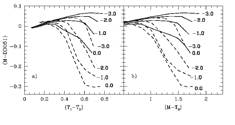
Figure 2: (a) The $(T_{1}-T_{2},M-DDO51)$ two-color diagram as invented by Geisler (1984), illustrated with the loci for giants solid lines and dwarfs dashed lines for the indicated values of [Fe/H], derived from the synthetic spectra generated by PB94. (b) Same as (a) but for the $(M-T_{2},M-DDO51)$ two-color plane adopted for our survey.

Paltoglou & Bell (1994, PB94 hereafter) demonstrated the gravity discrimination of Geisler’s system using a grid of synthetic spectra over a range of surface temperatures, gravities and abundances appropriate to both Population I and II stars, and including realistic sequences of atmospheres for red giant branch isochrones. Their work provides a useful demonstration of the effects of gravity and abundance on the ($M-DDO51$) index: gravity dominates the color but there is a secondary sensitivity to abundance. This is illustrated in Figure 2 where the PB94 synthetic colors are translated to loci in Washington/DDO51 color-color planes for dwarfs and giants of different [Fe/H].

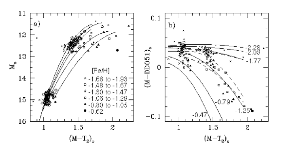
Figure 12: (a) $\omega$ Cen color-magnitude diagram for giant stars with radial velocity and proper motion membership as well as [Fe/H] determinations from Suntzeff & Kraft (1996). The latter chose stars from two magnitude ranges, one below and one above the horizontal branch. The legend describes the abundance groupings used for the giant stars. Second order fits to the RGBs of the various metallicity groupings are overplotted. The curves are in the order of abundance indicated in the panel legend, with abundance decreasing upward. The associated distribution in the two-color diagram is illustrated in panel (b). Second order fits to the two-color distributions for $\omega$ Cen giants of different metallicities, with the fits constrained by the color-color relations in PB94 (see text). The coefficients of the fits are given in Table 2. Note that the metallicities of the lines differ from those in panel (a) and Table 1; in panel (a) the intervals are set by the data from $\omega$ Cen alone, while in panel (b), we are constrained by the metallicity intervals chosen by PB94. The original empirical fits to the distribution of the (from top to bottom) [Fe/H]$=-1.74$, $-1.40$ and $-1.20$ groups are plotted in (b) (dashed lines) in order to illustrate the reasonable match obtained from the translated PB94 curves to the $\omega$ Cen data.

We note here one possible shortcoming of the PB94 curves: as noted by Lejeune & Buser (1996), PB94 used filter passbands which differ slightly from the adopted standard Washington filters, and furthermore, they have used an unpublished grid of model spectra, which are now somewhat out of date. This probably gives rise to the blueward translation and small rotation in the color-color plane that we find necessary in §3.6 (Figure 12b and Table 2). PB94 themselves point out that their isochrones are systematically redder than observed globular cluster giant branches. Unfortunately, Lejeune & Buser did not include the $DDO51$ filter when they produced their own (more accurate) synthetic colors. This leaves PB94 as the only source for synthetic photometry with which we can compare our own photometry. We emphasize that any problems with the PB94 colors appear to be quite small (again, see §3.6), in as much as they relate to our data.

Two important and relevant effects fall out of this interplay of gravity and abundance as illustrated in Figure 2. The first is that weakened absorption lines in metal-poor dwarfs that mimic the suppression of Mg absorption from low gravity in giants becomes a problem only for subdwarfs with [Fe/H]$\lesssim-2.5$. Main sequence stars more metal-rich than this, presumably all of those in the disk components and the majority in the halo as well, are not, in general, confused with giants, even giants as metal-rich as the Sun. The second relevant effect is that, for stars on the giant branch, the ($M-DDO51$) color provides a reasonably good abundance indicator [$(\partial(M-DDO51)/\partial\rm{[Fe/H]})\sim 0.13$ at ($T_{1}-T2=0.6$)] from solar [Fe/H] down to [Fe/H]$\sim-2.0$.

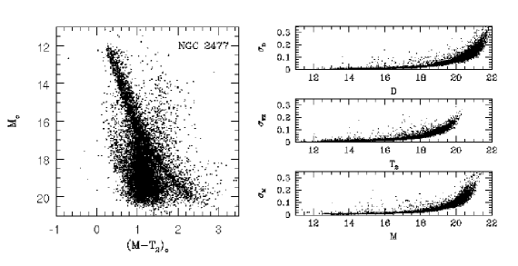
Figure 7: Color-magnitude diagram for 11,300 stars in the field of the open cluster NGC 2477, with near solar abundance. The field shows substantial, and probably variable, reddening, from $E(B-V)=0.2$ to $0.4$. The cluster is dereddened with the assumption of a mean $E(B-V)=0.33$. The scattering of stars upward from the main sequence is likely due to differential reddening in the field, and this is supported by the lessening of the effect on the lower main sequence, which more nearly parallels the reddening vector. The right hand panels show the random photometric errors in our catalogue.

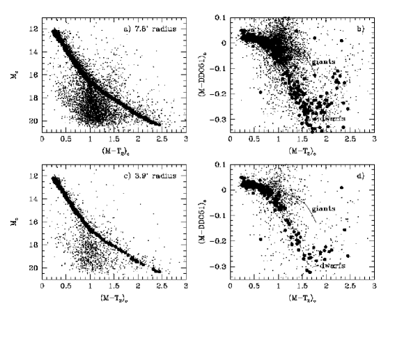
Figure 8: (a) Color-magnitude diagram for a more limited field of radius $7\farcm 8$ around the center of the open cluster NGC 2477. The large symbols are a “by eye” selection of the apparently least-reddened main sequence for the cluster. Without ancillary membership information, some field star contamination of this latter sample might be expected. The resultant ($M-T_{2}$)_o-($M-DDO51$)_o distribution of the selected sample is shown in (b). The PB94 lines for giants (solid) and dwarfs (dashed) of solar metallicity are also shown. (c) An even more restricted cut in radius around the center of the cluster, with radius $3\farcm 9$ around the cluster center. Again, we select by eye a representative least-reddened main sequence for the cluster, shown with large symbols. The stars in panel (c) are shown in the two-color distribution in (d). The PB94 solar metallicity lines from panel (b) are again plotted in (d). The distributions in both panels (b) and (d) suggest that the “by eye” selections are yielding mainly dwarf stars.

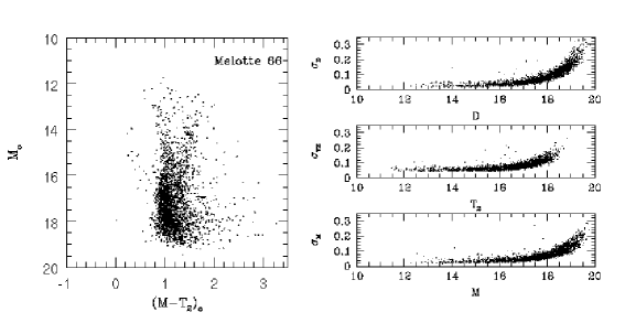
Figure 9: Color-magnitude diagram for the open cluster Melotte 66. Our catalogue contains 2643 stars from one telescope pointing. We adopt a reddening of $E(B-V)=0.16$ for the cluster. The right hand panels give the random errors in the photometry.

Both of these effects are critical to our enterprise here. First, the metallicity sensitivity of ($M-DDO51$) we expect to be useful for an initial sorting of faint giant stars we encounter. For example, the appearance of an apparent excess of giant stars of a single ($M-DDO51$)-based abundance would be an expected signal for a tidal tail from a mono-metallic parent object (a commonly expected paradigm). Such an excess is clearly seen, for example, in our study of extratidal stars near the Carina dwarf spheroidal galaxy in Paper II (see, e.g., Figures 7–9 in that paper).

In the case of very metal-poor subdwarfs, we should not encounter an overwhelming number of contaminants in a sample of giants selected by ($M-DDO51$) techniques, based on the very small fraction of Galactic stars with metallicities this poor. From the interim model of Reid & Majewski (1993), the number of halo intermediate Population II/thick disk stars expected in the $1\lesssim{M-T_{2}}\lesssim 2$ color range down to $V=20$ is about 200 deg^-2 at a Galactic pole. Approximately half of these stars would be dwarfs and only about 8% of these would be expected to have metallicities [Fe/H] $\lesssim 2.5$, according to Beers (1999) and Norris (1999). This leaves an expected level of contamination of $\sim 8$ metal-poor subdwarfs deg^-2, comparable to an expected density of giants of $\lesssim 9$ deg^-2 down to $V=20$. This is, of course, in the ideal situation of high Galactic latitude. On the other hand, because of the rapid decline in the metallicity distribution function below [Fe/H]$\sim-2.0$, it is possible, with only slightly more conservative giant selection in the color-color plane, to reduce the subdwarf contamination to practically nothing. For example, if one were interested in selecting for [Fe/H]$\lesssim-1$ giants, one would only be concerned with about two [Fe/H]$\lesssim-3$ subdwarfs per square degree (see Figure 2; Norris 1999).

We believe this level of contamination in our initial photometric catalogues to be tolerable. In any case, when such stars are encountered, they will be identifiable by followup spectra (or, for the brighter stars, by their proper motion from such catalogues as the NLTT; Luyten 1979, et seq.). Moreover, these metal-poor stars are interesting in their own right, and worthy of discovery for further exploration of the Galaxy’s evolution.

For our survey, we have adopted a variant of the Geisler technique that balances the goals of covering large areas as efficiently as possible with the desire to obtain as much information about identified giant stars as possible. We have adopted a three filter photometric system that provides dwarf/giant separation capability, a surface temperature indicator, and a rough gauge of stellar abundance in giant stars. In Geisler (1984), the $T_{1}-T_{2}$ color serves as a surface temperature index, while the $M-DDO51$ is used as the luminosity index. However, as we shall show (§2.1), the $M-T_{2}$ color is monotonically correlated to the $T_{1}-T_{2}$ color. Thus, $M-T_{2}$ can serve as a suitable temperature index (as has also been demonstrated by Geisler, Clariá & Minniti 1991), with the advantage that one less filter is needed in the observations with no loss in information – a useful improvement in efficiency. In this paper, we explore and calibrate the ($M-T_{2}$, $M-DDO51$) diagram for discriminating dwarf and giant stars for a range of metallicities (§2).

We note that the Washington $C$ filter is designed specifically for photometric abundance measurement in giant stars, and use of this filter would provide a much more accurate [Fe/H] for our survey giants (particularly metal-poor ones) than relying on the secondary dependence of ($M-DDO51$) on abundance. However, observations in the $C$ filter are rather expensive (requiring 3 times the exposure time of the $M$ filter to reach an equivalent depth – Canterna 1976). Since we already require a large investment in observing time for the $DDO51$ filter, and our primary imaging goal is to identify giants with as great efficiency as possible, we have dispensed with using the $C$ filter in most of what we do. Our rationale is two-fold: (1) We believe that the coarse abundances afforded by the ($M-DDO51$) color are sufficient for tidal tail/halo substructure searches in our photometry, and (2) it is our intention to back up our photometrically identified giant candidates with spectroscopy as much as possible. Spectroscopy is needed not only as a check on our giant candidates, but also as a means to obtain dynamical information from their radial velocities. Much better abundances may be obtained from moderate resolution spectra (sufficient for a radial velocity measure) than from $C$ filter photometry. Typical spectra of the type we are using for this followup work are shown in Figure 1, where several spectroscopic indicators of surface gravity, including the Mgb, MgH, and NaD features, may be seen. We will discuss our spectroscopic work for this survey further in future contributions.

1.3 Field Selection Strategy

The selection of fields for our survey reflects two distinct, but complementary, strategies. The first is predicated on the paradigm afforded by the example of the Sgr dwarf galaxy as well as by dynamical models of tidal effects on satellite galaxies (e.g., Johnston, 1998; Johnston et al., 1999), both which suggest that a non-negligible mass loss rate in the form of stripped stars may be discernible around presently known satellite galaxies. Thus, it makes sense to start a search for tidal tails in the Galactic halo at the most obvious potential sites for their creation. We have therefore begun a systematic search for giant stars beyond the tidal radii of the Galactic dwarf satellite galaxies, as well as a sample of globular clusters. We have already reported successful searches for extended, coherent stellar structures around our first two targets, the Magellanic Clouds (Majewski, 1999; Majewski et al., 1999a) and the Carina dwarf spheroidal (Paper II).

As the example of the Sgr galaxy illustrates, the tidal debris of satellite galaxies may stretch to substantial lengths (Mateo, Olszewski & Morrison 1998; Dinescu et al. 2000), and perhaps completely encircle the sky (Johnston et al., 1996; Johnston, 1998; Ibata et al., 2000). Tracing substantially lengthy tails continuously outward from the parent could be an extremely time-consuming enterprise, and should be weighed against the potential for tracking the path of the debris with more disparate, strategically placed, pencil beam probes around the sky. Another problem that may be addressed with a series of probes is the existence of debris from objects that no longer exist with any recognizable, gravitationally intact core. In terms of the formation history of the Milky Way halo, it is obviously of great interest to assess the net contribution of disrupted bodies to the halo. Finally, in order to understand the distribution of any “smooth background” of halo stars – the magnitude of which affects the contrast of any superimposed substructure (Johnston et al., 1996; Johnston, 1998) – it makes sense to perform a more systematic survey that can address the global distribution of giant stars.

For all of these reasons, and others, we have also embarked on the Grid Giant Star Survey (GGSS). The GGSS is a program to observe 1303 isotropically spaced (mean field spacing $\sim 5\fdg 6$) Galaxy pencil-beam probes, each of area 0.4–0.7 deg², to find giant and HB stars to explore Galaxy structure. The details and results of this systematic survey will be presented elsewhere. The “all-Galaxy” GGSS has similar goals and strategy to the “Spaghetti survey” described by Morrison et al. (2000). This survey also adopts a ($C,M,DDO51,T_{2}$) photometric search phase to identify giants and HB stars for spectroscopic followup, and has presented initial findings and discussion of strategy in Morrison et al. (2000). Together, the Spaghetti and GGSS surveys should provide a wealth of new information on the outer Galaxy.

In §2 we determine transformations from our ($M$, $T_{2}$) system to both the ($M$, $T_{1}$, $T_{2}$) and ($V$, $I$) systems. In §3 we calibrate the ($M-T_{2}$, $M-DDO51$) color-color diagram for discriminating dwarfs and giants, and explore the metallicity trends for giant stars in this diagram. We obtain good agreement in our empirical calibration of this two-color plane with that given by synthetic spectra. Finally, by way of $\omega$ Centauri giants as templates, we determine a rough calibration of giant star absolute magnitudes as a function of photometric abundance (i.e., position in the two-color diagram), which can be used for photometric parallaxes.

2 Photometric Transformations

2.1 $T_{1}-T_{2}$ to $M-T_{2}$

The Washington system was originally designed to obtain temperatures, metal abundances and CN indices (which relate well to [Fe/H] for Population I stars, Janes 1975, but vary independently of abundance for [Fe/H]$\lesssim{-0.75}$, Hartkopf & Yoss 1982) for G and K giants photometrically (Canterna, 1976). The primary goal of the photometric part of our survey is simpler – to identify potential giant stars. Thus, whenever possible, candidate giants will be subjected to spectroscopic follow-up to verify surface gravity (weeding out K subdwarfs), obtain a radial velocity and determine a spectroscopic metallicity. Thus, we can hope to reduce the number of Washington filter measurements to the minimum necessary to achieve our survey goals. For example, at present we are not emphasizing measurement of carbon abundances, so the CN and G band-sensitive $C$ filter is not essential to our aims. On the other hand, the $M$ filter is needed to serve as a “continuum” complement to the $DDO51$ filter, a l̀a Geisler (1984), and must be retained.

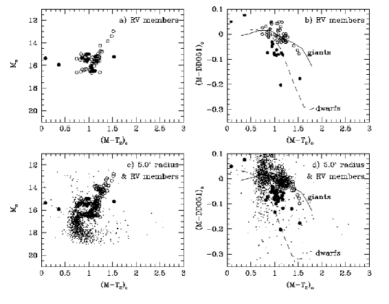
Figure 10: (a) Color-magnitude diagram for radial velocity members of Melotte 66 as determined by the sources cited in the text. The double subgiant branch of the cluster, a result of a high binary fraction, can be seen. The associated two-color distribution is given in (b), with the PB94 lines for giants (solid) and dwarfs (dashed) of solar metallicity also shown. The solid circles mark stars that seem to fall in unexpected regions for giant stars in the two-color diagram. A number of these seem to be members of the upper subgiant branch, and binarity may therefore be the cause for the observed deviation. Many of these “problem stars” also have abnormally large DAOPHOT $\chi$ values compared to other stars at the same magnitude. To clarify the MSTO and subgiant region of Melotte 66 we show all stars within $5\farcm 0$ of the cluster center in (c) and (d). Then, using the binary and single star isochrones in Kassis et al. (1997), as well as the known radial velocity Melotte 66 members in panel (a) – all of which are shown in (c) and (d) regardless of their radius from the cluster center – as guides, we trace out the pair of giant/subgiant branches to their respective main sequence turnoff points, showing the selected additional stars as large symbols. The dots are all remaining stars within $5\farcm 0$ of the cluster center. As in panels (a) and (b), we show “problem giant/subgiant” stars – those with unexpected colors in the two-color diagram – as solid circles. The latter seem to be more associated with the binary sequence. Panel (d) demonstrates how the two-color diagram becomes decreasingly effective as a surface gravity discriminator as the subgiant branch merges into the main sequence. The PB94 solar metallicity lines from panel (b) are again plotted in (d).

Because the sensitivity of the $M-DDO51$ index to surface gravity is a function of surface temperature, and because the derivation of spectroscopic abundances and gravities requires some measure of the effective temperature, we need an additional photometric measure sensitive to $T_{eff}$. In the standard Washington system, the $T_{1}-T_{2}$ parameter serves the role of a temperature index, but for our purposes greater efficiency could be obtained if a single additional filter could be combined with the already required $M$ filter to provide a suitable temperature index. Unfortunately, the $M$ filter is subjected to more line blanketing in metal-rich stellar atmospheres than the $T_{1}$ filter. Indeed, in the Washington system (Canterna, 1976), the combination of $M-T_{1}$ with $T_{1}-T_{2}$ is intended to provide a metallicity index, $\Delta(M-T_{1})$ (measured from the solar abundance locus – similar to the definition of $\delta(U-B)$). However, according to Figure 10 of (Canterna, 1976), the range of $\Delta(M-T_{1})$, is at most about 0.15 magnitudes over $0\geq$ [Fe/H] $\geq-2.5$ for giants with a wide range of $T_{1}-T_{2}$; and for giants with [Fe/H] $\leq-1.0$ – typical of the expected metallicities of distant giants we might hope to find in our survey – the range of $\Delta(M-T_{1})$ is only about 0.05 magnitudes. Thus, the $M-T_{2}$ color may provide an adequate temperature index for our purposes. Indeed, Lejeune & Buser (1996) conclude that “$M-T_{2}$ is better than $T_{1}-T_{2}$ for temperature determinations, although it is slightly sensitive to surface gravity.”

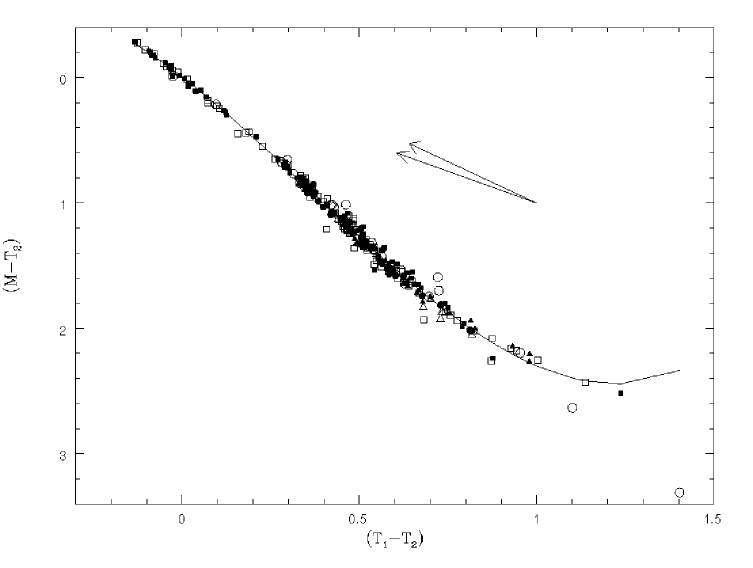
Figure 3: The $(M-T_{2})_{o}$ versus $(T_{1}-T_{2})_{o}$ plane using data from the sources cited in the text. Symbols denote luminosity classes, according to the legend in Figure 4. The upper reddening vector is from Canterna (1976), the lower one is taken from the analysis in §2.3. The solid line is a 4th order fit to the data, apart from the reddest two data points. The data include dwarfs and giants from a wide range of metallicities, is not corrected for reddening, and yet shows a relatively tight correlation of $M-T_{2}$ to $T_{1}-T_{2}$.

In Figure 3 we justify our exclusion of $T_{1}$ imaging in the present survey as a means to reduce our photometric survey to the simple $M,T_{2},DDO51$ filter system. Figure 3 shows all stars from Tables V and VII in Canterna (1976, open squares), Table VI of Harris & Canterna (1979, solid squares), Table III of Geisler (1984, symbols as in that paper: open triangles for luminosity class I-II, solid triangles for luminosity class III-IV, and solid circles for luminosity class V-VI), Table 2 of Geisler (1990, open circles), and solar abundance field giants from Table 1 of Geisler et al. (1991, solid triangles). Note, we exclude data for stars from Canterna (1976) when they were reobserved and updated in Harris & Canterna (1979), but we include both of the separate measures for the few stars repeated in Harris & Canterna (1979) and Geisler (1984), since these are separate data sets. Figure 3, which includes dwarfs and giants of a wide range of metallicities, and which has not been corrected for reddening, already demonstrates the relative tightness of the monotonic and almost (over most colors) linear $M-T_{2}$ versus $T_{1}-T_{2}$ correlation. The upper dereddening vector in this diagram is from Canterna (1976), while the lower one is based on the reddening ratios derived in §2.3 below. The solid line indicates a 4th order fit through the points, ignoring the two reddest $M-T_{2}$ stars from Geisler (1990), which are in highly reddened, Galactic plane fields. The root-mean-squared (RMS) scatter around the fit to this assortment of stars, without accounting for differing metallicities and reddening, is only 0.046 (or 0.036 when iteratively excluding greater than 3-$\sigma$ points).

We conclude that while $T_{1}-T_{2}$ has been proven an excellent $T_{eff}$ index for G and K stars (Canterna, 1976), the $M-T_{2}$ color also provides an adequate color index suitably correlated to $T_{eff}$ and with only slight sensitivity to abundances. That we can retain excellent dwarf-giant discrimination in the three filter $M,T_{2},DDO51$ system is illustrated by the synthetic photometry of PB94 in Figure 2b. In the remainder of this paper we provide an empirical formulation for this methodology.

2.2 Transformation of the ($M$, $T_{2}$) system to the ($V$, $I$) system

It is useful to determine the transformation of our Washington ($M$, $T_{2}$) filter system into the more commonly used Cousins ($V$, $I$) system. In this way we may compare our field star and cluster color-magnitude data to the extensive work done in the Cousins system in the literature.

To determine the transformation functions we take advantage of the tabulation of photometry by Harris & Canterna (1979), who have measured $V$ magnitudes along with Washington photometry in the establishment of their standard star system. We also make the assumption that the $T_{2}$ filter is identical to the Cousins $I_{C}$ filter. This assumption is justified by the great similarity of the $T_{2}$ bandpass described by Canterna (1976, see his Figure 1) and that of the Cousins $I_{C}$ band as illustrated by Bessell (1986, see his Figure 1). Indeed, both bands are often produced by the same combination of Schott RG-9 filter with dry-ice cooled Ga-As photomultiplier (Bessell, 1990), and similar effective filter central wavelengths, $\lambda_{eff}\approx 7885$ Å, are determined for giant star colors for the $T_{2}$ and $I_{C}$ filters by these two authors. However, as discussed by Bessell, the standard stars of Cousins (1981) were established with a photomultiplier kept $65\arcdeg$C warmer, which gives rise to a 130 Å redward shift in the $\lambda_{eff}$ in the Cousins standards. We ignore here any possible affect this might have on any $T_{2}$ to $I_{C}$ transformation. Presumably, the $T_{2}$ magnitudes of Harris & Canterna would be identical to the “natural GaAs” system $I_{C}$ band of Bessell (1986, see his Section III), from which Bessell notes a slight non-unity (a slope of 1.036) in conversion to the standard Cousins (1981) system in $(R-I)$ color, all attributed to the $I$ band shift with photomultiplier temperature. Thus, we might expect a systematic error in the slope of the ($M-T_{2}$) to $(V-I)_{C}$ color conversion derived below of up to 3.6%. Also to be kept in mind are any possible extensions of the redward side of the $I_{C}$ or $T_{2}$ response function for any combination of, say, the RG-9 glass (a “cut-on” filter) and CCD detectors that may have significant response up to the substrate bandgap cutoff in the near-infrared; this problem would affect the reddest stars.

For the 79 stars in Harris & Canterna (1979) that span $-0.285\leq(M-T_{2})\leq 2.518$, we obtain a good linear color transformation (RMS residual = 0.014) as follows:

$$(V-I)_{C}=(V_{C}-T_{2})=-0.006+0.800(M-T_{2}).$$ (1)

A significant contribution to the RMS residual about this fit was contributed by the two reddest stars, each having $M-T_{2}>2.02$, in the sample. A cubic fit to the data yields no significant improvement.

With the assumption $I_{C}=T_{2}$, we find from the above relation that $V_{C}$ may be determined by

$$V_{C}=M-0.006-0.200(M-T_{2}).$$ (2)

2.3 Selective Extinction Ratios

Because the objects we use to calibrate our ($M-T_{2}$, $M-DDO51$) diagram in §3 are typically at low Galactic latitudes, we must correct for extinction by dust. We adopt the average interstellar extinction curve for $R_{V}=A_{V}/E(B-V)=3.1$ of Savage & Mathis (1979). For the $M$ ($\lambda_{eff}=5085$ Å , $\lambda^{-1}=1.97\mu{m}^{-1}$, Canterna 1976) and $T_{2}$ ($\lambda_{eff}=7885$ Å , $\lambda^{-1}=1.24\mu{m}^{-1}$) filters we obtain $E(M-V)=0.33E(B-V)$ and $E(T_{2}-V)=-1.27E(B-V)$. Thus

$$E(M-T_{2})=1.60E(B-V),$$ (3)

compared with $E(M-T_{2})=1.59E(B-V)$ from Canterna & Harris (1979). Using older absorption curves, Canterna (1976) derived $E(M-T_{2})=1.67E(B-V)$.

The effective wavelength of the $DDO51$ filter yields $\lambda^{-1}=1.94\mu{m}^{-1}$, so that $E(DDO51-V)=0.27$. It follows that

$$E(M-DDO51)=0.06E(B-V).$$ (4)

We also find

$$A(M)=3.43E(B-V).$$ (5)

3 Calibration of the Magnesium Index

In this section, we demonstrate how we discriminate between giants and dwarfs in the $M-DDO51$ versus $M-T_{2}$ plane. Our demonstration utilizes both previous data in the literature, as well as new photometric data collected on the Swope 1-m telescope at Las Campanas Observatory. We also investigate the secondary dependence of the ($M-DDO51$) filter on [Fe/H].

3.1 Field Star Data from Geisler (1984)

In Figure 4 we show the $M-DDO51$ versus $M-T_{2}$ plane with data from Geisler (1984) and Geisler et al. (1991) (for solar metallicity field giants), where photometric data for stars with known luminosity class and reddening are provided. Figure 4 here is analogous to Geisler’s (1984) Figure 3. As can be seen, while there is little ability to discriminate between supergiants and giants, in general there is excellent discrimination between dwarfs and evolved stars of all luminosity classes I-III, as was suggested by the synthetic photometry presented in Figure 2b. For $M-T_{2}>1$, subgiants and dwarfs are also well discriminated, but, as might be expected, the separation begins to break down for bluer colors, near the main sequence turn off. With the new data presented here, we sample this important color regime with a large number of stars, with the aim of defining a useful guide for dwarf/giant demarcation in surveys of field stars.

3.2 New Observations of Star Clusters

Data for all of the star clusters presented here, except for Melotte 66, were obtained with the SITe #1 2048² CCD attached to the Swope 1-m on the nights of UT 15-17 March 1997. All but the very end of the last night of this run was photometric. The Melotte 66 data were obtained with the same filters, telescope and CCD on the photometric night of UT Dec. 15, 1997.

We used the “Carnegie 3-inch Washington Filter Set” to which we added a $DDO51$ filter. We believe that the Washington filters were purchased from Omega Optical and that the filters are based on the following prescription:

$M$ filter: 3 mm Schott GG-455 + 5 mm Corning CS-4-96, as prescribed by Canterna (1976).

$T_{2}$ filter: 9mm Schott RG-9

$DDO51$: The $DDO51$ filter was purchased from Omega Optical in 1993, as filter 515BP12, lot #9349. This filter is similar to the one described by Geisler (1984), but with a slightly larger peak transmission (88% versus Geisler’s 75%) and a very slightly narrower passband (half transmission at about 5095 Å and 5200 Å ).

Our cluster observations were calibrated with Geisler’s (1990) SA98, SA110, and NGC 3680 standard star fields, accounting for color, airmass, and, in the case of the $M$ band, (airmass) $\times$ (color) terms, along the lines of the procedure followed in Majewski et al. (1994b). For the $M$ and $T_{2}$ solutions, the ($M-T_{2}$) color was used, whereas, for the $DDO51$ solution, an ($M-DDO51$) color was used. For the first two nights of the March run, during which standard stars were measured, the solution was allowed to determine individual night zero-points, and these agreed to better than 0.013 in all cases. The extinction was assumed to be constant over all three March 1997 nights. In each of the $M$, $T_{2}$ and $DDO51$ solutions, there were 88, 69 and 64 useful standard stars, yielding solutions with RMS errors of 0.0036, 0.0051 and 0.0073 magnitudes, respectively.

3.3 NGC 3680

Our photometric catalogue for the intermediate aged (Anthony-Twarog et al., 1991) cluster NGC 3680 employed ten $M$, eight $T_{2}$ and nine $DDO51$ frames having integration times in the ranges of 5-8 seconds, 5-8 seconds and 50-90 seconds respectively. The images included Geisler’s (1984) calibration sequence in the Washington system. These CCD frames were reduced using DAOPHOT II (Stetson, 1994), calibrated and checked against Geisler’s sequence, and combined into a single catalogue. Our CCD frames cover $23\farcm 5$ per side, at $0\farcs 68$ per pixel.

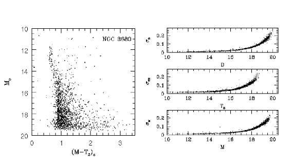
Figure 5: Color-magnitude diagram for our catalogue of 1815 stars in the field of the open cluster NGC 3680. Right hand panels show the random errors in the photometry in our three filters. Photometry is corrected under the assumption of $E(B-V)=0.046$.

In Figure 5 we present the ($M$, $M-T_{2}$) color-magnitude diagram (CMD) for 1815 stars in our CCD field of NGC 3680. Random errors in the photometry are presented in the right hand panels of Figure 5. We have adopted $E(B-V)=0.046$ (Nissen 1988, and consistent with Nordström, Andersen & Andersen 1997, NAA97 hereafter), and $A_{V}=0.143$, or $E(M-T_{2})=0.074$, $E(M-DDO51)=0.003$, and $A_{M}=0.158$. Friel & Janes (1993) determined the abundance of NGC 3680 to be [Fe/H]$=-0.16$, but an analysis of the CMD based on members cleaned of binary systems by NAA97 gives [Fe/H] = +0.11 (similar to the value of +0.09 $\pm 0.08$ of Nissen 1988) and an age of 1.45 $\pm$ 0.3 Gyr.

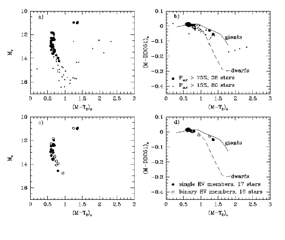
Figure 6: (a) Color-magnitude diagram for stars in our NGC 3680 catalogue also having proper motions by K95 most consistent with cluster membership. Large symbols denote stars with a high probability of membership, as evaluated by the joint proper motion-radius index, $P_{\mu,r}$, in their survey, while the small symbols indicate stars with less certain membership. (b) The ($M-T_{2}$)_o-($M-DDO51$)_o diagram for the same sample of stars. The PB94 lines for giants (solid) and dwarfs (dashed) of solar metallicity are also shown. (c) The $(M-T_{2},M)$ CMD for stars in our NGC 3680 catalogue also having precision radial velocity membership as determined by Nordström et al. (1997). Open symbols show radial velocity binary stars, whereas closed symbols show stars exhibiting no binarism in their radial velocities. (d) The ($M-T_{2}$)_o-($M-DDO51$)_o diagram for the radial velocity members of NGC 3680. The PB94 solar metallicity lines from panel (b) are again plotted.

A significant amount of field star contamination is evident in the NGC 3680 CMD, especially around $(M-T_{2})_{o}=1.0$, which is near the main sequence turn-off of old disk field stars ($(M-T_{2})_{o}\sim 0.85$). The latter overlap significantly the NGC 3680 main sequence stars of interest. We have cross-referenced our photometric catalogue to both the proper motion catalogue of Kozhurina-Platais et al. (1995, K95 hereafter) and to the radial velocity catalogue of NAA97. This allows us to separate true NGC 3680 members from the numerous field star contaminants, and also eliminate binary stars. In Figure 6a we show the CMD for only those stars having measured proper motions by K95 and with determined joint proper motion-spatial membership probability $P_{\mu,r}>15\%$. This low value was selected to mimic K95’s own selection (see Figure 8 in K95) and intended to preserve some fainter stars in the cluster CMD (faint stars tend to have lower $P_{\mu,r}$ in the K95 survey). However, as K95 point out, this liberal cut probably results in contamination of the lower main sequence by field stars (e.g., the proper motion errors in K95 begin to grow substantially for $B>15$). Therefore, with larger symbols we denote a more conservative cut with the K95 estimator cutoff at $P_{\mu,r}>75\%$. In Figure 6b we show the resultant ($M-T_{2}$)_o-($M-DDO51$)_o diagram for the proper motion selected samples.

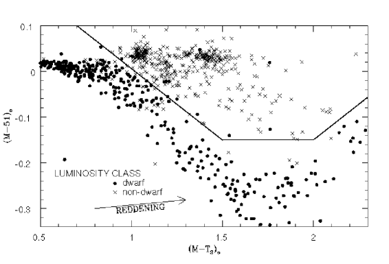
Figure 14: Summary ($M-T_{2}$)_o-($M-DDO51$)_o diagram of all giant and dwarf data discussed in this paper. The crosses represent giant stars presented in Figure 13, our red giants from NGC 3680 (both single and binary radial velocity members in Figure 6d) and $\omega$ Cen (Figure 12b), the red giant and subgiant branch of Melotte 66 (radial velocity members from the single star locus only, Figure 10b), the solar abundance field giants from Geisler et al. (1991), as well as all evolved stars from Geisler’s (1984) classes “IV-V” or class I. The solid circles (dwarfs) are Geisler (1984) luminosity class V and V-VI stars, and our open cluster main sequences from NGC 3680 (both single and binary radial velocity members in Figure 6d) and NGC 2477 (those stars selected as main sequence in Figure 8d). Giant stars (crosses) are, for most ($M-T_{2}$)_o colors, well separated from the dwarfs, for all metallicities. The straight solid lines roughly demarcate the region above which one might expect to find predominantly subgiant and giant stars.

Use of the much more refined membership analysis of NAA97, which employed precision radial velocities, clarifies the dwarf/giant discrimination by colors, albeit only for a bright subsample (Figures 6c and 6d). We include the high quality membership data of Figure 6d in Figure 14, below. Figure 6c looks qualitatively similar to NAA97’s ($b-y,V$) CMD for NGC 3680. It can be seen, from the general agreement of the points with the PB94 loci for [Fe/H]=0 stars, that the likely NGC 3680 giants, near $M_{o}=11.0$, as well as the likely main sequence stars more or less fall in the appropriate places in the color-color diagram.

3.4 NGC 2477

The rich open cluster NGC 2477 was observed in order to get a large sample of likely lower main sequence stars. Unfortunately, extending the cluster main sequence as faint as possible resulted in the saturation of our frames for a majority of the suspected cluster giants, which are lost from our analysis. We obtained two $M$, three $T_{2}$ and two $DDO51$ CCD exposures, for integrations of 60-80 seconds, 60 seconds, and 600 seconds each, respectively. Again DAOPHOT II was used to create a calibrated photometric catalogue. In Figure 7 we present the ($M$, $M-T_{2}$)_o CMD for 11,300 stars in the field of NGC 2477. Previous studies suggest the cluster shows substantial differential reddening, from $E(B-V)=0.2$ to 0.4 (Hartwick, Hesser & McClure, 1972); following Hartwick et al. (1972) and Smith & Hesser (1983), we have adopted a mean $E(B-V)=0.33$ and $A_{V}=0.99$. This translates to $E(M-T_{2})=0.53$, $E(M-DDO51)=0.02$ and $A_{M}=1.13$. The resultant CMD in Figure 7 is qualitatively identical with the $(V-I,V)$ CMD of Kassis et al. (1997), apart from the lack of a concentration of giants in our CMD. The broadening of the upper main sequence has been attributed to the differential reddening, and this is supported by the fact that the lower main sequence, which more nearly parallels the reddening vector, is thinner, particularly in the ($V-I,V$) CMD (Kassis et al., 1997).

Cluster parameters for NGC 2477 have most recently been determined by isochrone fitting in Kassis et al. (1997). This latter study finds best fits to [Fe/H] = $-0.05\pm 0.11$ and an age of $1_{-0.2}^{+0.3}$ Gyr. Earlier age estimates were slightly higher, e.g., 1.5 $\pm$ 0.2 Gyr (Hartwick et al., 1972) and 1.2 $\pm$ 0.3 Gyr (Smith & Hesser, 1983), but Carraro & Chiosi (1994), who used the same theoretical isochrones as Kassis et al. but on the Hartwick et al. data, obtained 0.6 $\pm 0.1$ Gyr. The white dwarf cooling curve age of the cluster tends to support the higher ages, around 1 Gyr (von Hippel, Gilmore & Jones, 1995). The best fitting Kassis et al. abundance for NGC 2477 is slightly lower, but not significantly so, from the [Fe/H]=0.04 value of Smith & Hesser (1983).

In spite of the amount of attention NGC 2477 has received lately by way of deep studies (von Hippel et al., 1995; Galaz et al., 1996), no membership study, even at the bright end of the CMD, exists for this cluster. In an attempt to improve our chances of selecting true NGC 2477 main sequence stars so that we might better delineate the dwarf locus in the ($M-T$, $M-D$)_o diagram, we reduce the field sample by limiting the CMD to stars in two specific radii – $7\farcm 8$ (Figures 8a-b) and $3\farcm 9$ (Figures 8c-d) – about the nominal cluster center (which was judged by finding the peak of the X and Y marginal distribution histogram of starcounts for $M<16$). By eye we selected stars along the apparently least-reddened NGC 2477 main sequence and show their position in the two-color diagram in Figures 8b and 8d (large dots). The small dots show a large population of apparent metal-rich field giants along the predicted PB94 [Fe/H]=0 giant locus, while the predicted trend for the selected dwarf sequence is clearly borne out by the data. The spreading of the locus at redder ($M-T_{2}$)_o colors is a consequence both of the increased photometric error for the fainter stars in the sequence as well the contribution of differential reddening, which increases as the dwarf sequence curves ever more perpendicular to the reddening vector in the lower part of the diagram. Note the much larger spread in the unselected stars in Figures 8b and 8d. This spread about the locus is partly due to large photometric errors at the faint limit of the catalogue (as high as 0.4 magnitudes in the colors). However, the larger bulk of stars above the dwarf locus hints at a substantial population of field giants in this low latitude ($b=-6^{o}$) field.

3.5 Melotte 66

Melotte 66 has long been recognized as an archetypal old open cluster (e.g., Hawarden, 1976). Recent studies estimate an age for the cluster of $4.5\pm 0.5$ Gyr (Twarog, Anthony-Twarog & Hawarden, 1995) and $4\pm 1$ Gyr (Kassis et al., 1997). Kassis et al. (1997) adopt an abundance of [Fe/H]=$-0.51\pm 0.11$, based on Friel & Janes (1993), which is similar to the adopted abundance ([Fe/H]=$-0.53\pm 0.08$) of Twarog et al. (1995). However, an intrinsic metallicity spread among the cluster giants has also been detected (Twarog et al., 1995). The reddening to the cluster does not seem well established, although Twarog et al. (1995) settle on $E(B-V)=0.16\pm 0.02$ as the reddening that gives the most consistent ultraviolet excesses between the cluster dwarfs and giants. We adopt this value, so that $E(M-T_{2})=0.26$, $E(M-DDO51)=0.01$ and $A_{M}=0.55$.

We obtained single $M$, $T_{2}$ and $DDO51$ exposures of Melotte 66 with integration times of 12, 12 and 100 seconds, respectively, for the Dec 1997 run. These were calibrated with 67, 59 and 60 useful standard stars in the $M$, $T_{2}$ and $DDO51$ bands, respectively, yielding solutions with random errors of 0.0094, 0.0074 and 0.0109 magnitudes, respectively. With these exposure times, we were able to get reliable photometry for all but the very brightest part of the red giant branch. We present in Figure 9 the CMD in our filter system for the field of Melotte 66. There is substantial field contamination, but the main sequence turn off region and the red clump of the cluster can be discerned easily.

While it is in somewhat better shape than either NGC 3680 or NGC 2477, Melotte 66 is still in need of a better membership census. Some radial velocity memberships exist and in Figures 10a and 10b we show those stars listed as members by Gratton (1982), Cameron & Reid (1987), Olszewski et al. (1991), Friel & Janes (1993) and from the Geisler & Smith (1984) analysis listed in Twarog et al. (1995). The result shows the prominent double CMD sequence caused by the substantial binary fraction in the cluster. This duplication causes both the double subgiant branches as well as a fattening of the MSTO region (see Figures 9 and 10c). We show the $(M-T_{2},M-DDO51)_{o}$ diagram corresponding to the identified members in Figure 10b. Here we delineate two groups of radial velocity member giants/subgiants: those falling more or less in the expected region of the color-color diagram (open circles) and those in more peculiar locations, more like expectations for dwarf stars (closed circles). It can be seen that the peculiarly-placed stars in Figure 10b seem to be predominantly associated with the upper subgiant branch, that of the binary stars, although a few stars, near $(M-T_{2})_{o}\approx 1.1$, are found below this subgiant branch. It may be that the wide scatter in $(M-DDO51)_{o}$ color near $M-T_{2}\approx 1.0$ in Figure 10b (and Figure 10d below), which gives rise to “problem giant stars” in the dwarf region of the two-color diagram, may be due to problems with the binarity. It is interesting also to note that many of these “problem stars” have abnormally large DAOPHOT $\chi$ parameters compared to other stars at similar magnitudes. Perhaps this is some indication of a slight resolution of close binaries that is detectable by DAOPHOT.

In Figures 10c and 10d, we attempt to elucidate the true nature of the red giant branch for the cluster by limiting our field to a radius of $5\farcm 0$. In Figure 10c we trace likely cluster members using the known radial velocity members (shown in Figure 10c whether or not they fall within the $5\farcm 0$ radius) and both the single and binary isochrones in Figure 9d of Kassis et al. (1997) as guides. Once again, we use open and closed circles to delineate stars with “problematical” colors from the standpoint of dwarf/giant separation. We trace down the red giant branch to the red clump and down the subgiant branch to the point where both the binaries and the single stars join their respective main sequence turnoffs. All other stars within $5\farcm 0$ of the cluster center are left as small symbols in Figures 10c and 10d. In Figure 10d the giants above the red clump follow the PB94 locus for solar metallicity giants. As expected (from, for example, Figure 4), the subgiant locus in Figure 10d merges with, and becomes less discriminated from, the locus of main sequence turnoff stars (small points) at bluer colors. The latter sweep lower than the main locus of giant stars in Figure 10d, as expected. Finally, we note again a predilection for the “giants” with problematical locations in the two-color diagram to be associated with the subgiant branch for binary members.

3.6 $\omega$ Centauri

Because of its proximity and size, $\omega$ Centauri is a convenient target that provides numerous bright giant stars for use as calibrators. Moreover, with an abundance ranging from solar to [Fe/H]$<-2.0$ (Butler et al., 1978; Persson et al., 1980; Suntzeff & Kraft, 1996), this one cluster allows the opportunity to explore the abundance sensitivity of the $M-DDO51$ index, as well as to calibrate the giant star color-magnitude relation as a function of metallicity for old stellar populations, without introduction of relative systematic errors produced by differential distance errors. To explore the giant distribution in the ($M-T_{2}$, $M-DDO51$) and the ($M-T_{2}$, $M$) planes, we have made an extensive imaging survey of the globular cluster $\omega$ Centauri.

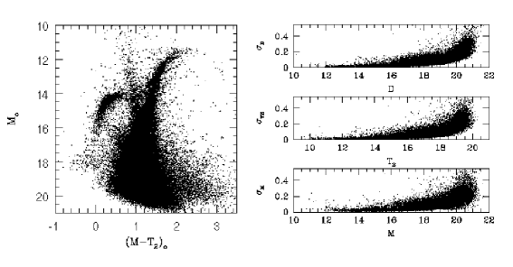
Figure 11: $\omega$ Cen color-magnitude diagram for over 100,000 stars in our catalogue generated from a $3\times 3$ grid of pointings around the cluster, less the central, saturated core. Some stars have been observed two or three times if they happened to fall in CCD frame overlap regions; these multiple detections have not been removed from the DAOPHOT catalogue or the diagram, which contain a quarter million entries. Some of the very reddest, highest luminosity giants have been lost due to saturation on the (fairly short) CCD integrations. The right hand panels give the random errors in the photometry. The vertical thickness in the error plots, compared with Figures 5, 7 and 9, is due to the fact that the individual pointings which make up the $\omega$ Cen database are not all to the same depth.

Our $\omega$ Cen data consists of eight separate pointings, offset by $15\farcm 3$ in each the North, South, East, West, Northeast, Northwest, Southeast, and Southwest directions. Our resulting catalogue contains over 100,000 stars photometered, in general, two or three times each, with DAOPHOT. The data were matched into catalogues using DAOMASTER. The Washington CMD for $\omega$ Centauri is presented in Figure 11. We have adopted $E(B-V)=0.15$ as in Suntzeff & Kraft (1996); this translates to $E(M-T_{2})=0.24$, $E(M-DDO51)=0.009$, and $A_{M}=0.51$. Two points are worth mentioning about Figure 11. First, as it is meant only for illustrative purposes, this figure has not yet been cleaned of multiple detections on overlapping frames, so that some stars appearing in overlap regions are represented two to three times. Second, because of saturation at the bright end, we have lost some of the very brightest, reddest $\omega$ Cen giants in this truncated CMD. An interesting aspect of Figure 11 is the appearance of several distinct RGBs, an aspect we explore further elsewhere (Majewski et al., 1999b).

We have cross-referenced our catalogue with the spectroscopic sample of Suntzeff & Kraft (1996). The latter is a careful analysis of abundance patterns in $\omega$ Cen giants, and also provides a membership list of 343 radial velocity members, stars that were selected in the first place as likely members based on proper motions. The stars studied by Suntzeff & Kraft were in two distinct magnitude ranges, one on the giant branch and one along the subgiant branch.

In Figure 12a, we show the distribution of the Suntzeff & Kraft giants in the ($M-T_{2}$, $M$)_o diagram, and in Figure 12b we show their distribution in the ($M-T_{2}$, $M-DDO51$)_o plane. Giants with different metallicity ranges are indicated by different symbols. The [Fe/H] ranges were selected so that the mean abundance in each metallicity bin corresponded to more or less convenient [Fe/H] values (-1.74, -1.60, -1.40, -1.20, -0.95) on the Norris & Da Costa (1995) abundance scale; the most metal-rich bin contains a single star at [Fe/H] = -0.62.

The distribution of points in Figure 12b demonstrates that while the $M-DDO51$ index is less sensitive to broad metallicity changes than it is to luminosity class differences (note the compressed range of $M-DDO51$ in Figure 12b), the ($M-T_{2}$, $M-DDO51$)_o plane is still able to discriminate roughly between metal-poor and metal-rich giants.

The $\omega$ Cen red giant branch is relatively well defined in Figure 11. A well defined RGB will be useful for our future studies, e.g., as a means to estimate rough photometric parallaxes for giants with Washington photometry. For each abundance, we fit the center of the RGB sequence analytically (using the IRAFtask CURFIT) to equations of the form

$$M_{o}=a+b(M-T_{2})_{o}+c(M-T_{2})_{o}^{2}$$ (6)

with the results given in Table 1, and plotted in Figure 12a.

To derive analytical descriptions of the rough abundance effect in the ($M-T_{2}$, $M-DDO51$)_o plane required several steps. We first fit the various metallicity bins with relations of the form

$$(M-DDO51)_{o}=d+e(M-T_{2})_{o}+f(M-T_{2})_{o}^{2}.$$ (7)

Especially at the extreme ends of the $\omega$ Cen abundance range, however, we found these fits to be unsatisfactorily constrained due to the small sample sizes, poor distribution in $(M-T_{2})$ color, and the contribution of photometric errors, which become larger than the mean separation of $(M-DDO51)$ colors for the metal-poor loci. The bimodal $(M-T_{2})$ distribution of the data gave rise to unlikely “bowing” between nodes fixed by the two concentration of points. Therefore, to give a more realistic and natural fit to the data, we have taken advantage of the synthetic curves derived for cluster CMDs by PB94, which we “calibrate” to our data for $\omega$ Cen. This forging of the synthetic loci to the actual data has the added advantage of extending the usefulness of the $\omega$ Cen example to abundance ranges outside those encompassed by the cluster itself, if we assume the relative placement of the synthetic loci is accurate. After trying various schemes to marry the synthetic and empirical loci, we found that we could obtain reasonable matches of the PB94 curves to the empirical distributions by metallicity with a simple 0.25 mag blueward translation (in $M-T_{2}$) and a slight ($<2\arcdeg$) rotation of the PB94 curves in the two-color plane. Thus we find

$$(M-T_{2})_{o}=(M-T_{2})_{o}^{PB94}-0.25,$$ (8)

and,

$$(M-DDO51)_{o}=(M-DDO51)_{o}^{PB94}-0.029*(M-T_{2})+0.03.$$ (9)

Note these relations are defined for the PB94 RGB 14 Gyr isochrones, and may not be applicable to their other models, and for clarity they were not considered in the previous discussion of the open clusters.

As pointed out in §1.2, the need to transform the PB94 relations is likely due to the nonstandard passbands adopted by PB94 (Lejeune & Buser, 1996), and it confirms the finding by PB94 that their isochrones are systematically redder than actual globular cluster red giant branches. Table 2 includes the original empirical fits to the metallicity bins in Table 1. We include only the [Fe/H]$=-1.74$, $1.40$ and $-1.20$ groups, which guided our transformation, in Figure 12b (dashed lines), along with the revised PB94 RGB loci (solid lines), and illustrates the reasonable matches of the latter to the $\omega$ Cen data. For future analytical ease the rotated PB94 loci have been fit by equations (7). The coefficients for these new relations are given in Table 2 for the various metallicities. The difference in the mean abundances for the listed loci in Table 2 compared to Table 1 is a result of our adopting the PB94 RGB curves (and therefore their abundance selections) for the latter.

To obtain the absolute magnitude, $M_{M}$ for a star using the relations in Table 1, one must correct the calculated apparent magnitude for the $\omega$ Cen distance modulus, which may be taken as (m-M)${}_{o}=13.57$ (Dickens et al., 1988), as well as the extinction in the $M$ band ($A_{M}=0.51$ for $E(B-V)=0.15$). It should be pointed out that since we have not been able to discriminate between first ascent red giant branch and asymptotic giant branch stars, the relations in Table 1 may tend to give systematically overluminous magnitudes if applied to individual first ascent giant branch stars. The ratio of first ascent to asymptotic giant branch stars in the brighter magnitude range in Figure 12a (i.e. above the horizontal branch) may be something like four to one (Suntzeff & Kraft, 1996). On the other hand, if the halo of the Galaxy evolved roughly similarly to $\omega$ Cen, with a similar age-metallicity relation and initial mass function, then we might expect a similar first ascent to asymptotic giant branch ratio in the field, and application of the Table 1 relations to finding distances for halo field stars should provide results that are at least statistically correct for an ensemble of giant stars.

3.7 Previously Published Data

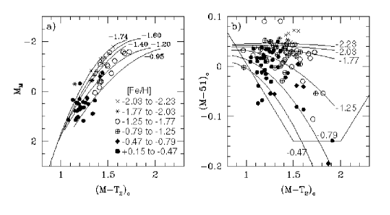
Figure 13: Summary of open and globular cluster data from sources in Table 3. (a) Color-magnitude diagram of open and globular cluster giants having $T_{1}$ magnitudes available from the Geisler collaboration for conversion to $M$ magnitudes. Distance moduli were adopted as given in Table 3, and we have assumed $R_{V}=A_{V}/E(B-V)=3.1$ and the reddening relations in §2.3. The iso-metallicity lines are from Figure 12a. (b) The resulting two-color diagram of the cluster giants from the data in Table 3, with the iso-metallicity lines from Figure 12b. For both panels (a) and (b) giant stars are grouped into metallicity bins indicated in panel (a). Note that the metallicity of the lines shown in panel (a) and panel (b) differ, as discussed in the caption for the previous figure. The straight solid lines in (b) are taken from those shown in Figure 14 below.

In a series of papers over more than a decade Doug Geisler and collaborators (Geisler 1986, 1987, 1988, Geisler, Clariá & Minniti 1991, 1992, 1997, Geisler, Minniti & Clariá 1992), have continued to refine calibration of the Washington photometry system through extensive observations of giant stars in open and globular clusters of all metallicities. In many cases, the Washington data presented have been supplemented with observations in the $DDO51$ filter as a means to discriminate cluster giants from foreground dwarfs. In Figure 13b we compile these data in the two-color diagram of interest to our analysis (similar to Figure 12b). Many of the stars were observed less frequently in $DDO51$ than in the other filters, and this has resulted in larger errors in the $M-DDO51$ color. Because of the sensitivity of the technique on relatively reliable $M-DDO51$ colors, we have excluded all stars which have fewer than three measures in $DDO51$. In Figure 13a we show the $(M-T_{2},M_{M})$ color-absolute magnitude diagram for those stars with available magnitude data in addition to colors.

Table 3 summarizes the data employed in the construction of Figure 13. In both Table 3 and Figure 13 the clusters are grouped according to [Fe/H] (with groups defined by the curves in Figure 13b), where the [Fe/H] and other data are from Mermilliod (1998) for the open clusters and from Harris (1998) for the globular clusters, with two exceptions: the distance moduli for NGC 2360 and NGC 6809 are taken from Mermilliod & Mayor (1990) and Alcaino et al. (1992), respectively. For these particular clusters the values listed in the databases of Mermilliod (1998) and Harris (1998) differ significantly from those in the literature (and we suspect an error in the databases). Figure 13 demonstrates that the general trends with [Fe/H] seen in the $\omega$ Cen giants are exhibited in the cluster giant population as a whole – namely, that the giants in the most metal-poor clusters show almost no variation of $(M-DDO51)$ color with $(M-T_{2})$, while more metal-rich cluster giants have progressively smaller $(M-DDO51)$, particularly at redder $(M-T_{2})$, as shown in Figure 12b. We have plotted the five color-color curves calibrated by the various metallicity populations in $\omega$ Cen (Table 2), with metallicity increasing towards the curves with smaller $(M-DDO51)$. We also include in Figure 13b the rough dwarf/giant demarcation (straight solid lines) recommended in the next Section. It may be seen that, apart from the very reddest and the very bluest stars, the majority of the giants lie above this demarcation line. The red upturn in the demarcating line is necessitated by the overlap with red dwarfs at $(M-T_{2})>2.0$ (see Figure 14) .

For a given abundance range the cluster data in Table 3, however, show much larger scatter in both Figure 13a and 13b compared to the $\omega$ Cen giants in Figures 12a and 12b. This is partly due to the heterogeneity in the sources and techniques employed to measure the fundamental parameters of distance, abundance and reddening for the Table 3 data. Of course, there is also a considerable spread in ages in the objects in Table 3, particularly with the inclusion of the open clusters, which contributes to the spreading of the distributions in Figure 13. In contrast, the PB94 isochrones we have used were derived from models with ages (14 Gyr) appropriate for globular cluster giant branches.

Because of the various problems with the heterogeneity of the data, we do not use Figure 13 to calculate general formulae for the conversion of color into absolute magnitude, as we did in Tables 1 and 2 for the $\omega$ Cen giants. We provide the Figure 13 data here to lend ancillary support to our assertion that rough abundance discrimination is possible in the $(M-T_{2},M-DDO51)$ diagram. While it would be nice to extend our Table 1 calibrations to higher abundances through inclusion of the metal-rich open clusters, for our present purposes there is no urgency for this since at the magnitudes and Galactic latitudes of our first applications of the technique we do not expect to encounter many giants with the metallicities and ages in the range of the metal-rich open clusters. We aim to return to this problem if and as needed.

We reiterate that much better photometric abundances can be had with inclusion of the Washington $C$ filter, as the numerous references listed in Table 3 can attest. However, our goal here is (1) to identify the minimal amount of photometric data necessary to find field giants that we have already begun to observe spectroscopically for radial velocities and, of course, abundances, and (2) to point out the additional leverage that our three color filter system has in characterizing the relative abundance of our giant star candidates.

3.8 Giant-Dwarf Discrimination

In Figure 14, we combine the two-color data of our open cluster main sequences from NGC 3680 (both single and binary radial velocity members in Figure 6d) and NGC 2477 (those stars selected as main sequence in Figure 8d), our red giants from NGC 3680 (both single and binary radial velocity members in Figure 6d) and $\omega$ Cen (Figure 12b), the red giant and subgiant branch of Melotte 66 (radial velocity members from the single star locus only, Figure 10b), the solar abundance field giants from Geisler et al. (1991), as well as the data on field dwarfs and giants from Geisler (1984), and giants from Geisler et al. (1991) (Figure 4) and the clusters listed in Table 3. All evolved stars, from Geisler’s single luminosity class “IV-V” to class I, are lumped into one group (“non-dwarfs”), as are all of the stars we show from the Melotte 66 red giant/subgiant branch. Note that Geisler (1984) specifically investigates the sensitivity of the $(M-DDO51)$ color to giants of different surface gravities and he finds little separation for giants of similar temperatures and metallicities but different log$g$.

We see that the discrimination of evolved stars and dwarfs is rather good over a broad range of $M-T_{2}$, breaking down only at the bluish colors ($M-T_{2}\approx 0.7-0.9$) of subgiant stars just evolved from the main sequence, and at the red end, starting around the colors of late K stars ($M-T_{2}\approx 2.3$), where overlap with dwarfs occurs again. The straight solid lines in the diagram roughly demarcate the region above which one might expect to find predominantly subgiant and giant stars. The “non-dwarf” objects that fall below these lines in Figure 14 are generally Geisler stars classified as subgiants, the lowest luminosity Melotte 66 subgiants, as well as the peculiar group of Melotte 66 stars (with $1.0\leq(M-T_{2})_{o}\leq 1.2$) discussed above.

The rather clear separation in Figure 14 motivates our survey for distant giant stars. With a 1-m class telescope and CCD imaging it is easy to obtain the photometric precision necessary to pick out rather complete samples of giant stars to distances of hundreds of kiloparsecs. By adopting this technique, we intend to explore the halo and local environment of the Milky Way and other galaxies in the Local Group with modest sized telescopes.

Table 1: Fits to $\omega$ Cen giant branches in the $(M-T_{2},M)_{o}$ color-magnitude diagram.

[Fe/H]	$\langle{\rm[Fe/H]}\rangle$	#stars	$(M-T_{2})_{o}$	$a$	$b$	$c$	RMS
$-$0.80 to $-$1.05	$-$0.95	10	1.14-2.05	25.3408	$-$12.2239	2.75723	0.242 (10)
$-$1.06 to $-$1.29	$-$1.20	18	1.04-1.95	25.9265	$-$13.9932	3.46823	0.236 (17)
$-$1.30 to $-$1.47	$-$1.40	31	1.01-1.69	27.6675	$-$16.5382	4.20810	0.196 (31)
$-$1.48 to $-$1.67	$-$1.60	76	0.98-1.85	29.5291	$-$19.3737	5.18975	0.231 (76)
$-$1.68 to $-$1.93	$-$1.74	91	0.85-1.94	31.7516	$-$22.9986	6.52318	0.206 (88)

Table 2: Fits to $\omega$ Cen giant stars in the $(M-T_{2},M-DDO51)_{o}$ color-color plane.

[Fe/H]	$d$	$e$	$f$
empirical curves
$-$1.20	$-$0.02598	+0.12815	$-$0.07806
$-$1.40	$-$0.14206	+0.31176	$-$0.13879
$-$1.74	+0.03193	+0.02258	$-$0.01605
synthesized curves
$-$0.47	$-$0.12560	+0.35652	$-$0.23447
$-$0.79	$-$0.08477	+0.27546	$-$0.17658
$-$1.25	$-$0.05076	+0.18657	$-$0.10393
$-$1.77	+0.01888	+0.04394	$-$0.02363
$-$2.03	+0.02907	+0.02549	$-$0.01225
$-$2.23	+0.02336	+0.03606	$-$0.01415

Table 3: Star clusters used in the construction of Figure 13.

Cluster			Global Cluster Data				Photometry Data
Name	Type		[Fe/H]	$E_{B-V}$	$(m-M)_{V}$		stars	reference
NGC 7099	globular		$-2.12$	0.03	14.57		14(6)	G88,GMC92
NGC 6809	globular		$-1.81$	0.07	14.10		15(6)	GMC92
NGC 6752	globular		$-1.55$	0.04	13.08		22(3)	GCM97
NGC 1904	globular		$-1.54$	0.01	15.53		11(1)	GCM97
NGC 1261	globular		$-1.35$	0.01	16.05		7(5)	G88
NGC 6121	globular		$-1.28$	0.36	12.78		23(12)	G86
NGC 1851	globular		$-1.26$	0.02	15.49		9(6)	GCM97
NGC 362	globular		$-1.16$	0.05	14.75		10(10)	G86
NGC 6723	globular		$-1.12$	0.05	14.82		13(13)	G86
NGC 6637	globular		$-0.71$	0.17	15.11		9(7)	G86
NGC 6352	globular		$-0.70$	0.21	14.39		19(1)	G86
NGC 2243	open		$-0.44$	0.03	13.17		6(6)	G87
NGC 2204	open		$-0.34$	0.08	13.44		8(8)	G87
Melotte 71	open		$-0.29$	0.01	12.53		9(7)	GCM92
NGC 2360	open		$-0.15$	0.09	10.30		6(6)	GCM92
NGC 6940	open		$+0.01$	0.23	10.83		10(10)	C86
NGC 6705	open		$+0.14$	0.42	12.61		22(6)	C86
NGC 6791	open		$+0.15$	0.18	13.93		12(2)	C86

References. — C86 – Canterna et al. (1986); G86 – Geisler (1986); G87 – Geisler (1987); G88 – Geisler (1988); GCM92 – Geisler, Clariá & Minniti (1992); GCM97 – Geisler, Clariá & Minniti (1997) – stars classed as dwarfs left out; GMC92 – Geisler, Minniti & Clariá (1992)

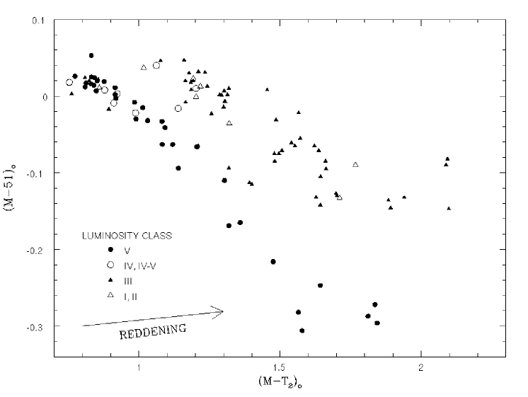
Figure 4: The $(M-DDO51)_{o}$ versus $(M-T_{2})_{o}$ plane using data from field stars from Geisler (1984) and solar abundance field giants from Geisler et al. (1991). Symbols denote luminosity classes as given in the legend. Figure 4 here is analogous to Geisler’s (1984) Figure 3, which shows the same general trends with luminosity class and color in the $(M-DDO51)_{o}$ versus $(T_{1}-T_{2})_{o}$ plane. While there is little ability to discriminate between supergiants and giants in our two color plane, there is excellent discrimination between dwarfs and evolved stars of luminosity classes I-III redward of $M-T_{2}$ colors typical of the main sequence turn off for old populations.

References

- Alcaino et al. (1992) Alcaino, G., Liller, W., Alvarado, F. & Wenderoth, E. 1992, AJ, 104, 190
- Anthony-Twarog et al. (1991) Anthony-Twarog, B. J., Heim, E. A., Twarog, B. A. & Caldwell, N. 1991, AJ, 102, 1056
- Arnold & Gilmore (1992) Arnold, R. & Gilmore, G. 1992, MNRAS, 257, 225
- Arp (1966) Arp, H. 1966, Atlas of Peculiar Galaxies, (Pasadena: California Institute of Technology)
- Ashman & Zepf (1992) Ashman, K. M. & Zepf, S. E. 1992, ApJ, 384, 50
- Bahcall & Soneira (1981) Bahcall, J. N. & Soneira, R. M. 1981, ApJS, 44, 73
- Beers (1999) Beers, T. C. 1999, in The Third Stromlo Symposium: The Galactic Halo, eds. B. K. Gibson, T. S. Axelrod & M. E. Putman, ASP Conf. Ser. Vol. 165, (San Francisco: ASP), 202
- Bessell (1986) Bessell, M. S. 1986, PASP, 98, 1303
- Bessell (1990) Bessell, M. S. 1990, PASP, 102, 1181
- Burkert (1997) Burkert, A. 1997, ApJ, 474, L99
- Butler et al. (1978) Butler, D., Dickens, R. J. & Epps, E. 1978, ApJ, 225, 148
- Cameron & Reid (1987) Cameron, A. C. & Reid, N. 1987, MNRAS, 224, 821
- Cannon et al. (1977) Cannon, R. D., Hawarden, T. G. & Tritton, S. B. 1977, MNRAS, 180, 81P
- Carney et al. (1996) Carney, B. W., Laird, J. B., Latham, D. W. & Aguilar, L. A. 1996, AJ, 112, 669
- Canterna (1976) Canterna, R. 1976, AJ, 81, 228
- Canterna & Harris (1979) Canterna, R. & Harris, H. C. 1979, AJ, 84, 1750
- Canterna et al. (1986) Canterna, R., Geisler, D., Harris, H. C., Olszewski, E. & Schommer, R. 1986, AJ, 92, 79 [C86]
- Carraro & Chiosi (1994) Carraro, G. & Chiosi, C. 1994, A&A, 287, 761
- Clark & McClure (1979) Clark, J. P. A. & McClure, R. D. 1979, PASP, 91, 507
- Côté et al. (1993) Côté, P., Welch, D. L., Fischer, P. & Irwin, M. J. 1993, ApJ, 406, L59
- Crane & Majewski (2000) Crane, J. D. & Majewski, S. R. 2000, in preparation
- Cousins (1981) Cousins, A. W. J. 1981, SAAO Circ., 1, No. 6, 4
- Dickens et al. (1988) Dickens, R.J., Brodie, I.R., Bingham, E.A. & Caldwell, S.P. 1988, Rutherford Appleton Laboratory, RAL 88-04
- Dinescu et al. (2000) Dinescu, D. I., Majewski, S. R., Girard, T. A. & Cudworth, K. M. 2000, AJ, accepted
- Doinidas & Beers (1989) Doinidas, S. P. & Beers, T. C. 1989, ApJ, 340, L57.
- Eggen (1960) Eggen, O. J. 1960, AJ, 65, 393
- Eggen (1977) Eggen, O. J. 1977, ApJ, 215, 812
- Eggen (1978) Eggen, O. J. 1978, ApJ, 221, 881
- Eggen (1996) Eggen, O. J. 1996, AJ, 112, 2661
- Eggen & Sandage (1959) Eggen, O. J. & Sandage, A. R. 1959, MNRAS, 119, 255
- Flynn & Freeman (1993) Flynn, C. & Freeman, K. C. 1993, A&AS, 96, 835
- Frenk et al. (1988) Frenk, C. S., White, S. D. M., Davis, M. & Efstathiou, G. 1988, ApJ, 327, 507
- Friel (1987) Friel, E. D. 1987, AJ, 93, 1388
- Friel & Janes (1993) Friel, E. D. & Janes, K. A. 1993, A&AS, 267, 75
- Fusi Pecci et al. (1995) Fusi Pecci, F., Bellazzini, M., Cacciari, C. & Ferraro, F. R. 1995, AJ, 110, 1664
- Galaz et al. (1996) Galaz, G., Ruiź, M. T., Thompson, I. & Roth, M. 1996, A&AS, 119, 413
- Geisler (1984) Geisler, D. 1984, PASP, 96, 723
- Geisler (1986) Geisler, D. 1986, PASP, 98, 847 [G86]
- Geisler (1987) Geisler, D. 1987, AJ, 94, 84 [G87]
- Geisler (1988) Geisler, D. 1988, PASP, 100, 687 [G88]
- Geisler (1990) Geisler, D. 1990, PASP, 102, 344
- Geisler et al. (1991) Geisler, D., Clariá, J. J. & Minniti, D. 1991, AJ, 102, 1836
- Geisler et al. (1992) Geisler, D., Clariá, J. J. & Minniti, D. 1992, AJ, 104, 1892 [GCM92]
- Geisler et al. (1997) Geisler, D., Clariá, J. J. & Minniti, D. 1997, PASP, 109, 799 [GCM97]
- Geisler et al. (1992) Geisler, D., Minniti, D. & Clariá, J. J. 1992, AJ, 104, 627 [GMC92]
- Geisler & Smith (1984) Geisler, D. P. & Smith, V. V. 1984, PASP, 96, 871
- Gould et al. (1992) Gould, A., Guhathakurta, P., Richstone, D. & Flynn, C. 1992, ApJ, 388, 345
- Governato et al. (1997) Governato, F., Moore, B., Renyue, C., Stadel, J., Lake, G. & Quinn, T. 1997, New Astronomy, 2, 91
- Gratton (1982) Gratton, R. G. 1982, ApJ, 257, 640
- Grebel (1997) Grebel, E. K. 1997, Rev. Mod. Astr., 10, 29
- Harris (1998) Harris, H. C. 1998, AJ, 112, 1487 (http://physun.physics.mcmaster.ca/GC/)
- Harris & Canterna (1979) Harris, H. C. & Canterna, R. 1979, AJ, 84, 1750
- Hartkopf & Yoss (1982) Hartkopf, W. I. & Yoss, K. M. 1982, AJ, 87, 1679
- Hartwick (1987) Hartwick, F. D. A. 1987, in The Galaxy: Proceedings of the NATO Advanced Study Institute, eds. G. Gilmore & B. Carswell, (Dordrecht: Reidel), 281
- Hartwick et al. (1972) Hartwick, F. D. A., Hesser, J. E. & McClure, R. D. 1972, ApJ, 174, 557
- Hawarden (1976) Hawarden, T. G. 1976, MNRAS, 174, 471
- Helmi & White (1999) Helmi, A. & White, S. D. M. 1999, MNRAS, 307, 495
- Helmi et al. (1999) Helmi, A., White, S. D. M., de Zeeuw, P. T. & Zhao, H. 1999, Nature, 402, 53
- Hunsberger et al. (1996) Hunsberger, S. D., Charlton, J. C. & Zaritsky, D. 1996, ApJ, 462, 50
- Ibata et al. (1995) Ibata, R. A., Gilmore, G. & Irwin, M. J. 1995, MNRAS, 277, 781
- Ibata & Irwin (1997) Ibata, R. A. & Irwin, M. J. 1997, AJ, 113, 1865
- Ibata et al. (2000) Ibata, R. A., Irwin, M., Lewis, G & Stolte, A. 2000, astro-ph/0004255
- Innanen & House (1970) Innanen, K. A. & House, F. C. 1970, AJ, 75, 680
- Irwin et al. (1990) Irwin, M. J., Bunclark, P. S., Bridgeland, M. T. & McMahon, R. G. 1990, MNRAS, 244, 16P
- Irwin et al. (1995) Irwin, M. J., Demers, S. & Kunkel, W. E. 1995, ApJ, 453, L21
- Janes (1975) Janes, K. A. 1975, ApJS, 29, 161
- Johnston (1998) Johnston, K. V. 1998, ApJ, 495, 297
- Johnston et al. (1996) Johnston, K. V., Hernquist, L. & Bolte, M. 1996, ApJ, 465, 278
- Johnston et al. (1999) Johnston, K. V., Sigurdsson, S. & Hernquist, L. 1999, MNRAS, 302, 771
- Kassis et al. (1997) Kassis, M., Janes, K. A., Friel, E. D. & Phelps, R. L. 1997, AJ, 113, 1723
- Kinman, Suntzeff & Kraft (1994) Kinman, T. D., Suntzeff, N. B. & Kraft, R. P. 1994, AJ, 108, 1722
- Klessen & Kroupa (1998) Klessen, R. S. & Kroupa, P. 1998, ApJ, 498, 143
- Kozhurina-Platais et al. (1995) Kozhurina-Platais, V., Girard, T. M., Platais, I., van Altena, W. F., Ianna, P. A. & Cannon, R. D. 1995, AJ, 109, 672 [K95]
- Kroupa (1997) Kroupa, P. 1997, New Astronomy, 2, 139
- Kuhn & Miller (1989) Kuhn, J. R. & Miller, R. H. 1989, ApJ, 341, L41
- Kunkel (1979) Kunkel, W. E. 1979, ApJ, 228, 718
- Kunkel & Demers (1976) Kunkel, W. E. & Demers, S. 1976, Roy. Greenwich Obs. Bull., 182, 241
- Lejeune & Buser (1996) Lejeune, T. & Buser, R. 1996 Baltic Astronomy, 5, 399
- Luyten (1979) Luyten, W. J. 1979, NLTT Catalogue I, (Minneapolis: University of Minnesota)
- Lynden-Bell (1982) Lynden-Bell, D. 1982, Observatory, 102, 202
- Lynden-Bell & Lynden-Bell (1995) Lynden-Bell, D. & Lynden-Bell, R. M. 1995, MNRAS, 275, 429
- Madore & Arp (1982) Madore, B. F. & Arp, H. C. 1982, PASP, 94, 40
- Majewski (1992) Majewski, S. R. 1992, ApJS, 78, 87
- Majewski (1993) Majewski, S. R. 1993, ARA&A, 31, 575
- Majewski (1994) Majewski, S. R. 1994, ApJ, 431, L17
- Majewski (1995) Majewski, S. R. 1995, in The Formation of the Milky Way, eds. E. J. Alfaro & A. J. Delgado (Cambridge: Cambridge University Press), 199.
- Majewski (1999) Majewski, S. R. 1999, in The Third Stromlo Symposium: The Galactic Halo, ASP Conf. Ser. Vol. 165, eds. B. K. Gibson, T. S. Axelrod & M. E. Putnam, (San Francisco: ASP), 76
- Majewski et al. (1994a) Majewski, S. R., Munn, J. A. & Hawley, S. L. 1994a, ApJ, 427, L37
- Majewski et al. (1994b) Majewski, S. R., Kron, R. G., Koo, D. C. & Bershady, M. A. 1994b, PASP, 106, 1258
- Majewski et al. (1996) Majewski, S. R., Munn, J. A. & Hawley, S. L. 1996, ApJ, 459, L73
- Majewski et al. (1999a) Majewski, S. R., Ostheimer, J. C., Kunkel, W. E., Johnston, K. V., Patterson, R. J. & Palma, C. 1999a, in IAU Symp. 190, New Views of the Magellanic Clouds, eds. Y.-H. Chu, J. Hesser & N. Suntzeff, (San Francisco: ASP), 171
- Majewski et al. (1999b) Majewski, S. R., Patterson, R. J., Dinescu, D. I., Johnson, W. Y., Ostheimer, J. C., Kunkel, W. E. & Palma, C. 1999b, astro-ph/9910278
- Majewski et al. (2000) Majewski, S. R., Ostheimer, J. C., Patterson, R. J., Kunkel, W. E., Johnston, K. V. & Geisler, D. 2000, AJ, 119, 760 [Paper II]
- Mateo et al. (1998) Mateo, M., Olszewski, E. W. & Morrison, H. L. 1998, ApJ, 508, L55
- McClure (1976) McClure, R. D. 1976, AJ, 81, 182
- McGlynn (1990) McGlynn, T. A. 1990, ApJ, 348, 515
- Mermilliod (1998) Mermilliod, J.-C. 1998, in Dynamical Studies of Star Clusters and Galaxies, eds. P. Kroupa, J. Palous & R. Spurzem (Noordwijk: ESA) (http://obswww.unige.ch/webda)
- Mermilliod & Mayor (1990) Mermilliod, J.-C. & Mayor, M. 1990, A&A, 237, 61
- Mihos & Bothun (1997) Mihos, J. C. & Bothun, G. D. 1997, ApJ, 481, 741
- Mirabel et al. (1992) Mirabel, I. F., Dottori, H. & Lutz, D. 1992, A&A, 256, L19
- Moore & Davis (1994) Moore, B. & Davis, M. 1994, MNRAS, 270, 209
- Morrison (1993) Morrison, H. L. 1993, AJ, 106, 578
- Morrison et al. (2000) Morrison, H. L., Mateo, M., Olszewski, E. W., Harding, P., Dohm-Palmer, R. C., Freeman, K. C., Norris, J. E. & Morita, M. 2000, AJ, 119, 2254
- Nemec & Nemec (1993) Nemec, J. M. & Nemec, A. F. L. 1993, AJ, 105, 1455
- Nissen (1988) Nissen, P. E. 1988, A&A, 199, 146
- Nordström et al. (1997) Nordström, B., Andersen, J. & Andersen, M. I. 1997, A&A, 322, 460 [NAA97]
- Norris (1994) Norris, J. E. 1994, ApJ, 431, 645
- Norris (1999) Norris, J. E. 1999, in The Third Stromlo Symposium: The Galactic Halo, eds. B. K. Gibson, T. S. Axelrod & M. E. Putman, ASP Conf. Ser. Vol. 165, (San Francisco: ASP), 213
- Norris & Da Costa (1995) Norris, J. E. & Da Costa, G. S. 1995, ApJ, 447, 680
- O’Connell (1958) O’Connell, D. J. K. 1958, ed., Ricerche Astronomiche, Specola Vaticana (New York: Interscience)
- Ohman (1934) Ohman, Y. 1934, ApJ, 80, 405
- Olszewski et al. (1991) Olszewski, E. W., Schommer, R. A., Suntzeff, N. B. & Harris, H. C. 1991, AJ, 101, 515
- Oort (1965) Oort, J. 1965 in Galactic Structure, eds. A. Blauuw & M. Schmidt, (Chicago: University of Chicago), 455
- Palma et al. (2000) Palma, C., Majewski, S. R. & Johnston, K. V. 2000, ApJ, submitted
- Paltoglou & Bell (1994) Paltoglou, G. & Bell, R. A. 1994, MNRAS, 268, 793 [PB94]
- Persson et al. (1980) Persson, S. E., Cohen, J. G., Matthews, K., Frogel, J. A. & Aaronson, M. 1980, ApJ, 235, 452
- Ratnatunga & Freeman (1983) Ratnatunga, K. U. & Freeman, K. C. 1983, IAU Colloquium 78, Astronomy with Schmidt-Type Telescopes, ed. M. Capaccioli, (Dordrecht: Reidel), 261
- Ratnatunga & Freeman (1985) Ratnatunga, K. U. & Freeman, K. C. 1985, ApJ, 291, 260
- Ratnatunga & Freeman (1989) Ratnatunga, K. U. & Freeman, K. C. 1989, ApJ, 339, 126
- Reid et al. (1996) Reid, I. N., Yan, L., Majewski, S., Thompson, I. & Smail, I. 1996, AJ, 112, 1472
- Reid & Majewski (1993) Reid, N. & Majewski, S. R. 1993, ApJ, 409, 635
- Robin & Crézé (1986) Robin, A. C. & Crézé, M. 1986, A&A, 157, 71
- Rodgers et al. (1990) Rodgers, A. W., Harding, P. & Walker, I. 1990, AJ, 100, 1841
- Saha (1985) Saha, A. 1985, ApJ, 289, 310
- Savage & Mathis (1979) Savage, B. D. & Mathis, J. S. 1979, ARA&A, 17, 73
- Schweizer et al. (1996) Schweizer, F., Miller, B. W., Whitmore, B. C. & Fall, S.M. 1996, AJ, 112, 1839
- Smecker-Hane et al. (1994) Smecker-Hane, T. A., Stetson, P. B., Hesser, J. E. & Lehnert, M. D. 1994, AJ, 108, 507
- Smith & Hesser (1983) Smith, H. A. & Hesser, J. E. 1983, PASP, 95, 277
- Sommer-Larsen & Christensen (1987) Sommer-Larsen, J. & Christensen, P. R. 1987, MNRAS, 225, 499
- Stetson (1994) Stetson, P. B. 1994, PASP, 106, 250
- Suntzeff & Kraft (1996) Suntzeff, N. B. & Kraft, R. P. 1996, AJ, 111, 1913
- Thackeray (1939) Thackeray, A. D. 1939, MNRAS, 99, 492
- Toomre & Toomre (1972) Toomre, A. & Toomre, J. 1972, ApJ, 178, 623
- Tremaine (1993) Tremaine, S. 1993, in Back to the Galaxy, eds. S. S. Holt & F. Verter, (New York: AIP Conference Proceedings), 599
- Tripicchio et al. (1997) Tripicchio, A., Severino, G., Covino, E., Terranegra, L. & García López, R. J. 1997, A&A, 327, 681
- Twarog et al. (1995) Twarog, B. A., Anthony-Twarog, B. J. & Hawarden, T. G. 1995, PASP, 107, 1215
- Valtonen et al. (1993) Valtonen, M. J., Byrd, G. G., McCall, M. L. & Innanen, K. A. 1993, AJ, 105, 886
- van den Bergh et al. (1996) van den Bergh, S., Abraham, R. G., Ellis, R. S., Tanvir, N. R., Santiago, B. X. & Glazebrook, K. G. 1996, AJ, 112, 359
- van de Rydt et al. (1991) van de Rydt, F., Demers, S. & Kunkel, W. E. 1991, AJ, 102, 130
- von Hippel et al. (1995) von Hippel, T., Gilmore, G. & Jones, D. H. P. 1995, MNRAS, 273, L39
- Yoss & Hartkopf (1979) Yoss, K. M. & Hartkopf, W. I. 1979, AJ, 84, 1293
- Yoss, Neese & Hartkopf (1987) Yoss, K. M., Neese, C. L. & Hartkopf, W. I. 1987, AJ, 94, 1600
- Zaritsky et al. (1989) Zaritsky, D., Olszewski, E. W., Schommer, R. A., Peterson, R. A. & Aaronson, M. 1989, ApJ, 345, 759