Stellar Evolution with Rotation V: Changes in all the Outputs of Massive Star Models

Abstract

Grids of models for rotating stars are constructed in the range of 9 to 120 M_⊙ at solar metallicity. The following effects of rotation are included: shellular rotation, new structure equations for non–conservative case, surface distorsions, increase of mass loss with rotation, meridional circulation and interaction with horizontal turbulence, shear instability and coupling with thermal effects, advection and diffusion of angular momentum treated in the non–stationary regime, transport and diffusion of the chemical elements.

Globally we find that for massive stars the effects of rotation have an importance comparable to those of mass loss. Due to meridional circulation the internal rotation law $\Omega(r)$ rapidly converges, in 1–2 % of the MS lifetime, towards a near equilibrium profile which then slowly evolves during the MS phase. The circulation shows two main cells. In the deep interior, circulation rises along the polar axis and goes down at the equator, while due to the Gratton–Öpik term it is the inverse in outer layers. This external inverse circulation grows in depth as evolution proceeds. We emphasize that a stationary approximation and a diffusive treatment of meridional circulation would be unappropriate. After the MS phase, the effects of core contraction and envelope expansion dominate the evolution of the angular momentum.

The surface velocities decrease very much during the MS evolution of the most massive stars, due to their high mass loss, which also removes a lot of angular momentum. This produces some convergence of the velocities, but not necessarily towards the break–up velocities. However, stars with masses below $\sim$12 M_⊙ with initially high rotation may easily reach the break–up velocities near the end of the MS phase, which may explain the occurence of Be–stars. Some other interesting properties of the rotational velocities are pointed out.

For an average rotation, the tracks in the HR diagram are modified like a moderate overshoot would do. In general, an average rotation may increase the MS lifetime up to about 30 %; for the helium–burning phase the effects are smaller and amount to at most 10 %. From plots of the isochrones, we find that rotation may increase the age estimate by about 25 % in general. However, for stars with M $\mathbin{\;\raise 1.0pt\hbox{$>$}\kern-8.0pt\lower 3.0pt\hbox{$\sim$}\;}$40 M_⊙ and fast rotation, a bluewards “homogeneous–like” track, with important He– and N–enrichments, may occur drastically affecting the age estimates for the youngest clusters. Rotation also introduces a large scatter in the mass–luminosity relation: at the same $\log g_{\rm eff}$ and $\log T_{\rm eff}$, differences of masses by 30 % may easily occur, thus explaining what still remains of the alleged mass discrepancy.

Rotation also brings significant surface He– and N–enhancements, they are higher for higher masses and rotation. While it is not difficult to explain very fast rotators with He– and N–excesses, the present models also well account for the many OB stars exhibiting surface enrichments and moderate or low rotation, (cf. Herrero et al. He92 (1992), He20 (2000)). These stars likely result from initially fast rotators, which experienced mixing and lost a lot of angular momentum due to enhanced mass loss. The comparison of the N–excesses for B– and A–type supergiants supports the conclusion by Venn (1995a , Ve99 (1999)), that these enrichments mostly result from mixing during the MS phase, which is also in agreement with the results of Lyubimkov (Lyu96 (1996)).

1 Introduction

Due to the many well known successes of the standard theory of stellar evolution, rotation has generally been considered as a secondary effect. This was justified in many cases. However, since some years a number of very significant discrepancies between model predictions and observations have been found for massive stars, and also for red giants of lower masses. These difficulties have been listed and examined (cf. Maeder 1995a ). Recently, large excesses of [N/H] have been found in A–type supergiants, particularly in the SMC (Venn et al. Ve98 (1998); Venn Ve99 (1999)), where the excesses may reach up to an order of magnitude with respect to the average [N/H] local value in the SMC. These excesses, not predicted by current models, are the signatures of mixing effects over the entire star. This extensive mixing changes the size of the reservoir of nuclear fuel available for evolution, and thus the lifetimes, the tracks and all the model outputs (cf. also Langer 1992; Langer 1997; Heger et al. 2000). Also the chemical abundances, the yields and the final stages may be modified. Rotation appears as a natural driver for this mixing or, at least, as one of the first mechanisms whose consequences for mixing has to be explored. This is especially true for massive stars which are known to be fast rotators (see e.g. Penny 1996; Howarth et al. 1997).

The physical effects of stellar rotation are numerous. The basic equations of stellar structure need to be modified. The meridional circulation and its interaction with the horizontal turbulence, the diffusion effects produced by shear turbulence, the inhibition of the transport mechanisms by the $\mu$–gradients, the transport of the angular momentum and of the chemical elements, the loss of mass and angular momentum at the surface, the enhancement of mass loss by rotation, etc…  are some of the effects to be included in realistic models. In addition to the model physics, rotation also brings a number of new numerical problems in the stellar code, such as the 4^th order equation for the transport of the angular momentum, which has to be coupled to the equations of stellar structure.

In this work, we apply the investments in the treatment of the physical and numerical effects of rotation made in the previous works and we explore their consequences for the outputs of stellar models. In Sect. 2, we describe the various effects considered. The non–rotating stellar models are briefly discussed in Sect. 3. The evolution of the internal rotation during the evolution is examined in Sect. 4. Sect. 5 discusses the effects of rotation on the evolutionary tracks in the HR diagram, on the lifetimes and isochrones. The evolution of the rotational velocities at the stellar surface is discussed in Sect. 6 and the effects on the surface abundances are analysed in Sect. 7.

2 Physical ingredients of the models

Let us briefly summarize here the basic physical ingredients of the numerical models of rotating stars we are constructing here.

2.1 Shellular rotation

The differential rotation which results from the evolution and transport of the angular momentum as described by Eq. (3) below, makes the stellar interior highly turbulent. The turbulence is very anisotropic, with a much stronger geostrophic–like transport in the horizontal direction than in the vertical one (Zahn Za92 (1992)), where stabilisation is favoured by the stable temperature gradient. This strong horizontal transport is characterized by a diffusion coefficient $D_{\rm{h}}$, which is quite large as will be shown below. The horizontal turbulent coupling favours an essentially constant angular velocity $\Omega$ on the isobars. This rotation law, constant on shells, applies to fast as well as to slow rotators. As an approximation, it is often represented by a law of the form $\Omega=\Omega(r)$ (Zahn Za92 (1992); see also Endal and Sofia ES76 (1976)).

2.2 Hydrostatic effects

In a rotating star, the equations of stellar structure need to be modified (Kippenhahn and Thomas KippTh70 (1970)). The usual spherical coordinates must be replaced by new coordinates characterizing the equipotentials. The classical method applies when the effective gravity can be derived from a potential $\Psi=\Phi-\frac{1}{2}\Omega^{2}r^{2}\sin^{2}\theta$, i.e. when the problem is conservative. There, $\Phi$ is the gravitational potential which in the Roche approximation is $\Phi=-\frac{GM_{r}}{r}$. If the rotation law is shellular, the problem is non–conservative. Most existing models of rotating stars apply, rather inconsistently, the classical scheme by Kippenhahn and Thomas. However, as shown by Meynet and Maeder (MM97 (1997)), the equations of stellar structure can still be written consistently, in term of a coordinate referring to the mass inside the isobaric surfaces. Thus, the problem of the stellar structure of a differentially rotating star with an angular velocity $\Omega=\Omega(r)$ can be kept one–dimensional.

2.3 Surface conditions

The distribution of temperature at the surface of a rotating star is described by the von Zeipel theorem (vZ24 (1924)). Usually, this theorem applies to the conservative case and states that the local radiative flux $\@vec{F}$ is proportional to the local effective gravity $\@vec{g_{\rm eff}}$, which is the sum of the gravity and centrifugal force,

$$\@vec{F}=-\frac{L(P)}{4\pi GM_{\star}(P)}\,\@vec{g_{\rm eff}}\;,$$ (1)

with $M_{\star}(P)=M(1-\frac{\Omega^{2}}{2\pi G\bar{\rho}})$; $L(P)$ is the luminosity on an isobar and $\bar{\rho}$ the mean internal density. The local $T_{\rm eff}$ on the surface of a rotating star varies like $T_{\rm eff}(\vartheta)\sim g_{\rm eff}(\vartheta)^{\frac{1}{4}}$. We define the average stellar $T_{\rm eff}$ by $T_{\rm eff}^{4}=L/(\sigma S(\Omega))$, where $\sigma$ is Stefan’s constant and $S(\Omega)$ the total actual stellar surface. Of course, for different orientation angles $i$, the emergent luminosity, colours and spectrum will be different (Maeder and Peytremann MP70 (1970)). In the case of non–conservative rotation law, the corrections to the von Zeipel theorem depend on the opacity law and on the degree of differential rotation, but they are small, i.e. $\leq 1\%$ in current cases of shellular rotation (Kippenhahn Kipp77 (1977); Maeder Mae99 (1999)). Wether or not the star is close to the Eddington limit, the von Zeipel theorem keeps the same form as the one given by Maeder (1999, see also Maeder & Meynet 2000a ). In this last work, it is in particular shown that the expression for the Eddington factor in a rotating star needs to be consistently written and that it contains a term depending on rotation.

2.4 Changes of the mass loss rates $\dot{M}$ with rotation

Observationally, a growth of the mass flux of OB stars with rotation, i.e. by 2–3 powers of 10, was found by Vardya (Var85 (1985)), while Nieuwenhuijzen and de Jager (Nieu88 (1988)) concluded that the $\dot{M}$–rates seem to increase only slightly with rotation for O– and B–type stars. On the theoretical side, Friend and Abbott (1986) find an increase of the $\dot{M}$–rates which can be fitted by the relation (Langer La98 (1998))

$$\dot{M}(v)\;=\;\dot{M}(v=0)\left(\frac{1}{1-\frac{v}{v_{\rm crit}}}\right)^{\xi}$$ (2)

with $\xi\simeq 0.5$ and $v_{\rm crit}$ the equatorial velocity at break–up. This expression is used in most evolutionary models and this is also what is done in the present work. The critical rotation velocity of a star is often written as $v^{2}_{\rm{crit}}=\frac{GM}{R_{\rm eb}}(1-\Gamma)$, where $R_{\rm eb}$ is the equatorial radius at break–up velocity and $\Gamma=L/L_{\rm{Edd}}$ is the ratio of the stellar luminosity to the Eddington luminosity (cf. Langer 1997, 1998). Glatzel (1998) has shown that when the effect of gravity darkening is taken into account, the above expression for $v_{\rm{crit}}$ does not apply. Glatzel (1998) gives $v^{2}_{\rm{crit}}=\frac{GM}{R_{\rm eb}}$, which we adopt here. The problem is now being further examined by Maeder & Meynet (2000a), who critically discuss the Eddington factors, their dependence on rotation, the expression of the critical velocity, the dependence of the mass loss rates on rotation. These various new results will be applied in subsequent works, particularly for the study of the effects of rotation on the formation of W–R stars. Further improvements, based either on the observations or on the theory, to account for the anisotropic winds which selectively remove the angular momentum need also to be performed.

The above expression gives the change of the mass loss rates due to rotation. As reference mass loss rates in the case of no rotation, we use the recent data by Lamers and Cassinelli (LaCa96 (1996)); for the domain not covered by these authors we use the results by de Jager et al. (Ja88 (1988)). During the Wolf–Rayet phase we use the mass loss rates proposed by Nugis et al (1998) for the WNL stars (mean, clumping–corrected rates from radio data $\dot{M}({\rm WNL})=3\ 10^{-5}$ M_⊙ y^-1). For the WNE and WC stars we use the prescription devised by Langer (1989), modified according to Schmutz (1997) for taking into account the clumping effects in Wolf-Rayet stellar winds ($\dot{M}=2.4\cdot 10^{-8}(M/{\rm M}_{\odot})^{2.5}$ M_⊙ y^-1). These mass loss rates are smaller by a factor 2–3 than the mass loss rates used in our previous stellar grids (Schaller et al. 1992; Meynet et al. 1994).

2.5 Transport of the angular momentum

For shellular rotation, the equation of transport of angular momentum in the vertical direction is in lagrangian coordinates (cf. Zahn Za92 (1992); Maeder and Zahn MZ98 (1998))

$$\rho\frac{d}{dt}\left(r^{2}\Omega\right)_{M_{r}}=$$ (3)

$$\frac{1}{5r^{2}}\frac{\partial}{\partial r}\left(\rho r^{4}\Omega U(r)\right)+\frac{1}{r^{2}}\frac{\partial}{\partial r}\left(\rho Dr^{4}\frac{\partial\Omega}{\partial r}\right).$$

$\Omega(r)$ is the mean angular velocity at level $r$. The vertical component $u(r,\theta)$ of the velocity of the meridional circulation at a distance $r$ to the center and at a colatitude $\theta$ can be written

$$u(r,\theta)=U(r)P_{2}(\cos\theta),$$ (4)

where $P_{2}(\cos\theta)$ is the second Legendre polynomial. Only the radial term $U(r)$ appears in Eq. (3). The quantity $D$ is the total diffusion coefficient representing the various instabilities considered and which transport the angular momentum, namely convection, semiconvection and shear turbulence. As a matter of fact, a very large diffusion coefficient as in convective regions implies a rotation law which is not far from solid body rotation. In this work, we take $D=D_{\rm{shear}}$ in radiative zones, since as extra–convective mixing we consider shear mixing and meridional circulation. In case the outward transport of the angular momentum by the shear is compensated by an inward transport due to the meridional circulation, we obtain the local conservation of the angular momentum. We call this solution the stationary solution. In this case, $U(r)$ is given by (cf. Zahn Za92 (1992))

$$U(r)=-\frac{5D}{\Omega}\frac{\partial\Omega}{\partial r}\;.$$ (5)

The full solution of Eq. (3) taking into account $U(r)$ and $D$ gives the non–stationary solution of the problem. In this case, $\Omega(r)$ evolves as a result of the various transport processes, according to their appropriate timescales, and in turn differential rotation influences the various above processes. This produces a feedback and, thus, a self–consistent solution for the evolution of $\Omega(r)$ has to be found.

The transport of angular momentum by circulation has often been treated as a diffusion process (Endal and Sofia ES76 (1976); Pinsonneault et al. Pin89 (1989); Heger et al. He00 (2000)). From Eq. (3), we see that the term with $U$ (advection) is functionally not the same as the term with $D$ (diffusion). Physically advection and diffusion are quite different: diffusion brings a quantity from where there is a lot to other places where there is little. This is not necessarily the case for advection. A circulation with a positive value of $U(r)$, i.e. rising along the polar axis and descending at the equator, is as a matter of fact making an inward transport of angular momentum. Thus, we see that when this process is treated as a diffusion, like a function of $\frac{\partial\Omega}{\partial r}$, even the sign of the effect may be wrong.

The expression of $U(r)$ given below (Eq. 12) involves derivatives up to the third order, thus Eq. (3) is of the fourth order, which makes the system very difficult to solve numerically. In practice, we have applied a Henyey scheme to make the calculations. Eq. (3) also implies four boundary conditions. At the stellar surface, we take (cf. Talon et al. Ta97 (1997); Denissenkov et al. Den99 (1999))

$$\frac{\partial\Omega}{\partial r}=0\;\;\;\;\mathrm{and}\;\;\;\;U(r)=0$$ (6)

and at the edge of the core we have

$$\frac{\partial\Omega}{\partial r}=0\;\;\;\;\mathrm{and}\;\;\;\;\Omega(r)=\Omega_{\mathrm{core}.}$$ (7)

We assume that the mass lost by stellar winds is just embarking its own angular momentum. This means that we ignore any possible magnetic coupling, as it occurs in low mass stars. This is not unreasonable in view of the negative results about the detection of magnetic fields in massive stars (Mathys Math99 (1999)). It is interesting to mention here, that in case of no viscous, nor magnetic coupling at the stellar surface, i.e. with the boundary conditions (6), the integration of Eq. (3) gives for an external shell of mass $\Delta M$ (Maeder 1999, paper IV)

$$\Delta M{d\over dt}(\Omega r^{2})=-{4\pi\over 5}\rho r^{4}\Omega U(r).$$ (8)

This equation is valid provided the stellar winds are spherically symmetric (see paper IV), an assumption we do in this work. When the surface velocity approches the critical velocity, it is likely that there are anisotropies of the mass loss rates (polar ejection or formation of an equatorial ring) and thus the surface condition should be modified according to the prescriptions of Maeder (Mae99 (1999)). For now, these effects are not included in these models. Their neglect should not affect too much the results presented here since the critical velocity is reached only in some rare circumstances.

2.6 Mixing and transport of the chemical elements

A diffusion–advection equation like Eq. (3) should normally be used to express the transport of chemical elements. However, if the horizontal component of the turbulent diffusion $D_{\rm{h}}$ is large, the vertical advection of the elements can be treated as a simple diffusion (Chaboyer and Zahn Cha92 (1992)) with a diffusion coefficient $D_{\rm eff}$. As emphasized by Chaboyer and Zahn, this does not apply to the transport of the angular momentum. $D_{\rm eff}$ is given by

$$D_{\rm eff}=\frac{\mid rU(r)\mid^{2}}{30D_{h}}\;,$$ (9)

where $D_{\rm{h}}$ is the coefficient of horizontal turbulence, for which the estimate is

$$D_{\mathrm{h}}\simeq|rU(r)|$$ (10)

according to Zahn (1992). Eq. (8) expresses that the vertical advection of chemical elements is severely inhibited by the strong horizontal turbulence characterized by $D_{\rm{h}}$. Thus, the change of the mass fraction $X_{i}$ of the chemical species $i$ is simply

$$\left(\frac{dX_{i}}{dt}\right)_{M_{r}}=$$ (11)

$$\left(\frac{\partial}{\partial M_{r}}\right)_{t}\left[(4\pi r^{2}\rho)^{2}D_{\rm mix}\left(\frac{\partial X_{i}}{\partial M_{r}}\right)_{t}\right]+\left(\frac{dX_{i}}{dt}\right)_{\rm nucl}.$$

The second term on the right accounts for composition changes due to nuclear reactions. The coefficient $D_{\rm mix}$ is the sum $D_{\rm mix}=D_{\rm shear}+D_{\rm eff}$ and $D_{\rm eff}$ is given by Eq. (9). The characteristic time for the mixing of chemical elements is therefore $t_{\rm mix}\simeq\frac{R^{2}}{D_{\rm mix}}$ and is not given by $t_{\rm circ}\simeq\frac{R}{U}$, as has been generally considered (Schwarzschild 1958). This makes the mixing of the chemical elements much slower, since $D_{\rm eff}$ is very much reduced. In this context, we recall that several authors have reduced by large factors, up to 30 or 100, the coefficient for the transport of the chemical elements, with respect to the transport of the angular momentum, in order to better fit the observed surface compositions (cf. Heger et al. He00 (2000)). This reduction of the diffusion of the chemical elements is no longer necessary with the more appropriate expression of $D_{\rm eff}$ given here.

When the effects of the shear and of the meridional circulation compensate each other for the transport of the angular momentum (stationary solution, see Sect. 2.5), the value of $U$ entering the expression for $D_{\rm eff}$ is given by Eq. (5).

2.7 Meridional circulation

Meridional circulation is an essential mixing mechanism in rotating stars and there is a considerable litterature on the subject (see ref. in Tassoul Tass90 (1990)). The velocity of the meridional circulation in the case of shellular rotation was derived by Zahn (Za92 (1992)). The effects of the vertical $\mu$–gradient $\nabla_{\mu}$ and of the horizontal turbulence on meridional circulation are very important and they were taken into account by Maeder and Zahn (MZ98 (1998)). Contrarily to the conclusions of previous works (e.g. Mestel Mes65 (1965); Kippenhahn and Weigert KippW90 (1990); Vauclair Vau99 (1999)), the $\mu$–gradients were shown not to introduce a velocity threshold for the occurence of the meridional circulation, but to progressively reduce the circulation when $\nabla_{\mu}$ increases. The expression by Maeder and Zahn (MZ98 (1998)) is

$$U(r)=\frac{P}{{\rho}{g}C_{\!P}{T}\,[\nabla_{\rm ad}-\nabla+(\varphi/\delta)\nabla_{\mu}]}$$ (12)

$$\ \ \ \ \ \ \ \ \ \left\{\frac{L}{M_{\star}}(E_{\Omega}+E_{\mu})\right\}\;.$$

$P$ is the pressure, $C_{P}$ the specific heat, $E_{\Omega}$ and $E_{\mu}$ are terms depending on the $\Omega$– and $\mu$–distributions respectively, up to the third order derivatives and on various thermodynamic quantities (see details in Maeder and Zahn, MZ98 (1998)). The term $\nabla_{\mu}$ in Eq. (12) results from the vertical chemical gradient and from the coupling between the horizontal and vertical $\mu$–gradients due to the horizontal turbulence. This term $\nabla_{\mu}$ may be one or two orders of magnitude larger than $\nabla_{\rm ad}-\nabla$ in some layers, so that $U(r)$ may be reduced by the same ratio. This is one of the important differences introduced by the work by Maeder and Zahn (MZ98 (1998)). Another difference is that the classical solution usually predicts an infinite velocity at the interface between a radiative and a semiconvective zone with an inverse circulation in the semiconvective zone. Expression (12) gives a continuity of the solution with no change of sign from semiconvective to radiative regions. Finally, we recall that in a stationary situation, $U(r)$ is given by Eq. (5), as seen above.

2.8 Shear turbulence and mixing

In a radiative zone, shear due to differential rotation is likely to be a most efficient mixing process. Indeed shear instability grows on a dynamical timescale that is of the order of the rotation period (Zahn Za92 (1992)). The usual criterion for shear instability is the Richardson criterion, which compares the balance between the restoring force of the density gradient and the excess energy present in the differentially rotating layers,

$$Ri=\frac{N^{2}_{\mathrm{ad}}}{(0.8836\ \Omega\frac{d\ln\Omega}{d\ln r})^{2}}<\frac{1}{4},$$ (13)

where we have taken the average over an isobar, $r$ is the radius and $N_{\rm{ad}}$ the Brunt-Väisälä frequency given by

$$N^{2}_{\rm{ad}}=\frac{g\delta}{H_{P}}\left[\frac{\varphi}{\delta}\nabla_{\mu}+\nabla_{ad}-\nabla_{\rm{rad}}\right].$$ (14)

When thermal dissipation is significant, the restoring force of buoyancy is reduced and the instability occurs more easily, its timescale is however longer, being the thermal timescale. This case is referred to as “secular shear instability”. The criterion for low Peclet numbers $Pe$ (i.e. of large thermal dissipation, see below) has been considered by Zahn (Za74 (1974)), while the cases of general Peclet numbers $Pe$ have been considered by Maeder (1995b ), Maeder and Meynet (MM96 (1996)), who give

$$Ri=\frac{g\delta}{(0.8836\ \Omega\frac{d\ln\Omega}{d\ln r})^{2}H_{P}}$$ (15)

$$\ \ \ \ \ \ \ \ \left[\frac{\Gamma}{\Gamma+1}(\nabla_{ad}-\nabla)+\frac{\varphi}{\delta}\nabla_{\mu}\right]<\frac{1}{4}$$

The quantity $\Gamma=Pe/6$, where the Peclet number $Pe$ is the ratio of the thermal cooling time to the dynamical time, i.e. $Pe=\frac{v\ell}{K}$ where $v$ and $\ell$ are the characteristic velocity and length scales, and $K=(4acT^{3})/(3C_{P}\kappa\rho^{2})$ is the thermal diffusivity. A discussion of shear–driven turbulence by Canuto (Ca98 (1998)) suggests that the limiting $Ri$ number may be larger than $\frac{1}{4}$.

To account for shear transport and diffusion in Eqs. (3) and (11), we need a diffusion coefficient. Amazingly, a great variety of coefficients $D_{\mathrm{shear}}=\frac{1}{3}v\ell$ have been derived and applied, for example:

– 1. Endal and Sofia (ES78 (1978)) apply the Reynolds and the Richardson criterion by Zahn (Za74 (1974)). They estimate $D_{\mathrm{shear}}$ from the product of the velocity scale height of the shear flow and of the turbulent velocities of cells at the edge of Reynolds critical number.

– 2. Pinsonneault et al. (Pin89 (1989)) notice that the amount of differential rotation permitted by the secular shears is proportional to a critical number, which they treat as an adjustable parameter. To account for the effects of the $\mu$–gradient in mixing, of the loss of angular momentum, etc… they introduce several adjustable parameters in the equations for the transport of the chemical elements and of the angular momentum.

– 3. Chaboyer et al. (1995a ) use a coefficient derived from the velocity and path length from Zahn (Za74 (1974)). Following Pinsonneault et al. (Pin89 (1989)), they also introduce two adjustable parameters for adjusting the transports of chemical elements and angular momentum respectively. We notice that thanks to the reduction of the diffusion produced by the horizontal turbulence (cf. Eq. 9 above), it is no longer necessary to arbitrarily reduce the vertical transport of the chemical elements.

– 4. Zahn (Za92 (1992)) defines the diffusion coefficient corresponding to the eddies which have the largest $Pe$ number so that the Richardson criterion is just marginally satisfied. However, the effects of the vertical $\mu$–gradient are not accounted for and the expression only applies to low Peclet numbers.

– 5. The same has been done by Maeder and Meynet (MM96 (1996)), who considers also the effect of the vertical $\mu$–gradient, the case of general Peclet numbers and, in addition they account for the coupling due to the fact that the shear also modifies the local thermal gradient. This coefficient has been used by Meynet and Maeder (MM97 (1997)) and by Denissenkov et al. (Den99 (1999)).

– 6. The comparisons of model results and observations of surface abundances have led many authors to conclude that the $\mu$–gradients appear to inhibit the shear mixing too much with respect to what is required by the observations (Chaboyer et al. 1995a b; Meynet and Maeder MM97 (1997); Heger et al. He00 (2000)). Namely, the observations of O–type stars (Herrero et al. He92 (1992), He99 (1999)) show much more He– and N–enrichments than predicted by the models which apply Richardon’s criterion with the $\nabla_{\mu}$ term. Thus, instead of using a gradient $\nabla_{\mu}$ in the criterion for shear mixing, Chaboyer et al. (1995a ) and Heger et al. (He00 (2000)) write $f_{\mu}\nabla_{\mu}$ with a factor $f_{\mu}=0.05$ or even smaller. This procedure is not satisfactory since it only accounts for a small fraction of the existing $\mu$–gradients in stars. The problem is that the models depend at least as much (if not more) on $f_{\mu}$ than on rotation, i.e. a change of $f_{\mu}$ in the allowed range (between 0 and 1) produces as important effects as a change of the initial rotational velocity. This situation has led to two other more physical approaches discussed below. Also Heger et al. (2000) introduce another factor $f_{c}$ to adjust the ratio of the transport of the angular momentum and of the chemical elements like Pinsonneault et al. (1989).

– 7. Talon and Zahn (TZ97 (1997)) account for the horizontal turbulence, which has a coefficient $D_{\rm{h}}$ and which weakens the restoring force of the gradient of $\mu$ in the usual Richardson criterion. This allows some mixing of the chemical elements to occur as required by the observations (Talon et al. Ta97 (1997)).

– 8. Indeed, around the convective core in the region where the $\mu$–gradient inhibits mixing, there is anyway some turbulence due to both the horizontal turbulence and to the semiconvective instability, which is generally present in massive stars. This situation has led to the hypothesis (Maeder Mae97 (1997)) that the excess energy in the shear, or a fraction $\alpha$ of it of the order of unity, is degraded by turbulence on the local thermal timescale. This progressively changes the entropy gradient and consequently the $\mu$–gradient. This hypothesis leads to a diffusion coefficient $D_{\rm shear}$ given by

$$D_{\rm shear}=4\frac{K}{N^{2}_{\rm{ad}}}\left[\frac{1}{4}\alpha\left(0.8836\ \Omega\frac{d\ln\Omega}{d\ln r}\right)^{2}-(\nabla^{\prime}-\nabla)\right].$$ (16)

The term $\nabla^{\prime}-\nabla$ in Eq. (16) expresses either the stabilizing effect of the thermal gradients in radiative zones or its destabilizing effect in semiconvective zones (if any). When the shear is negligible, $D_{\rm shear}$ tends towards the diffusion coefficient for semiconvection by Langer et al. (La83 (1983)) in semiconvective zones. When the thermal losses are large ($\nabla^{\prime}=\nabla$), it tends towards the value

$$D_{\rm shear}=\alpha(K/N^{2}_{\rm{ad}})\left(0.8836\ \Omega\frac{d\ln\Omega}{d\ln r}\right)^{2},$$ (17)

given by Zahn (Za92 (1992)). Eq. (16) is completed by the three following equations expressing the thermal effects (Maeder Mae97 (1997))

$$D_{\rm shear}=2K\Gamma\;\;\;\;\;\;\;\;\nabla=\frac{\nabla_{rad}+(\frac{6\Gamma^{2}}{1+\Gamma})\nabla_{ad}}{1+(\frac{6\Gamma^{2}}{1+\Gamma})},$$ (18)

$$\nabla^{\prime}-\nabla=\frac{\Gamma}{\Gamma+1}(\nabla_{\mathrm{ad}}-\nabla).$$ (19)

The system of 4 equations given by Eqs. (16), (18) and (19) form a coupled system with 4 unknown quantities $D$, $\Gamma$, $\nabla$ and $\nabla^{\prime}$. The system is of the third degree in $\Gamma$. When it is solved numerically, we find that as a matter of fact the thermal losses in the shears are rather large in massive stars and thus that the Peclet number $Pe$ is very small (of the order of 10^-3 to 10^-4, see Sect. 4.2). For very low Peclet number $Pe=6\Gamma$, the differences $(\nabla^{\prime}-\nabla)$ are also very small as shown by Eq. (19). Thus, we conclude that Eq. (16) is essentially equivalent, at least in massive stars, to the original Eq. (17) above, as given by Zahn (Za92 (1992)). We may suspect that this is not necessarily true in low and intermediate mass stars since there the $Pe$ number may be larger. Of course, the Reynolds condition $D_{\rm shear}\geq\frac{1}{3}\nu Re_{c}$ must be satisfied in order that the medium is turbulent. The quantity $\nu$ is the total viscosity (radiative + molecular) and $Re_{c}$ the critical Reynolds number estimated to be around 10 (cf. Denissenkov et al. Den99 (1999); Zahn Za92 (1992)). The numerical results in Sect. 4 will show the values of the various parameters and also indicate that the conditions for the occurence of turbulence are satisfied.

The physical treatment around the core also depends on the choice of the criterion for convection. In current literature, there are at least three basic sets of assumptions: a) Ledoux criterion, which leads to small cores, b) Schwarzschild’s criterion, which gives “medium size” cores, c) Schwarzschild’s criterion and overshooting, which gives large cores. Here, we choose to apply the intermediate solution b), which means that the above equation 16 is only applied in fully radiative regions. Some consequences of this choice of convective criterion are discussed in Sect. 3 below.

2.9 Initial compositions, opacities, nuclear reactions and other model ingredients

For purpose of comparison, we adopted here the same physical ingredients as for the solar metallicity models computed by Meynet et al. (me94 (1994)). The only exceptions, apart from the inclusion of the effects induced by rotation described above, are the following: we use the Schwarzschild criterion for convection without overshooting and the mass loss rates are as indicated in Sect. 2.4.

3 The non–rotating stellar models

For comparison purpose, we have computed non–rotating stellar models with exactly the same physical ingredients as the rotating ones. The corresponding evolutionary tracks and lifetimes are presented in Fig. 8 and Table 1. These stellar models have similar properties as older ones computed with the Schwarzschild criterion for convection. For instance, our non–rotating 9 M_⊙ stellar model has similar H– and He–burning lifetimes as the 9 M_⊙ model computed with the Schwarzschild criterion by Bertelli et al. (1985). Our models also well agree with more recent computations. Indeed our MS lifetimes are similar within about two percents to the ones obtained by Heger et al. (2000) for their non–rotating stellar models. These authors used the Ledoux criterion with semiconvection. However, since during the MS phase the convective core mass decreases, one expects, for this phase, only small differences between the models computed with the Ledoux and the Schwarzschild criterion. These comparisons show that the present non–rotating stellar models well agree with results obtained with different stellar evolutionary codes.

Many papers (e.g. Bertelli et al. 1985; Maeder & Meynet 1989; Chin & Stothers 1990; Langer & Maeder 1995; Canuto 2000) have discussed the effects of different criteria for convection on massive star evolution. Since our main aim in this paper is to emphasize the effects of rotation, we shall restrict ourselves to briefly mention some differences with previous grids of models computed by the Geneva group.

In the present non–rotating stellar models, computed without overshooting, the convective core masses are smaller than in the models by Schaller et al. (1992) and Meynet et al. (1994). As a consequence, the stars evolve at smaller luminosities. The turn–off point at the end of the MS occurs for higher T_eff and lower luminosities, reducing the extent of the MS width. The MS lifetimes are reduced. For initial masses below about 25 M_⊙, the He–burning lifetime is increased implying an increase of the ratio $t_{\rm He}/t_{\rm H}$ of the lifetimes in the He– and H–burning phases. For the higher initial masses, the effects of the stellar winds become very important and dominate the effects due to a change of the criterion for convection.

As a numerical example, in our non–rotating 20 M_⊙ stellar model, the convective core mass is reduced by 1–1.2 M_⊙ during the whole H–burning phase compared to its value given by Meynet et al. (1994). At the end of the MS phase, the mass of the helium core has decreased by $\sim$ 20% with respect to its value in models with a moderate overshoot. The position of the turn–off point has a $\log L$/L_⊙ decreased by 0.05 dex and a $\log T_{\rm eff}$ increased by 0.04 dex. The MS lifetime is decreased by about 10%, the ratio $t_{\rm He}/t_{\rm H}$ passes from 10% in the models of Meynet et al. (1994) to 14% in the present case.

4 The evolution of the internal rotation law $\Omega(r)$

4.1 The initial convergence of the rotation law

Let us first mention that even in some recent works the assumption of solid body rotation is often considered. However, it is much more physical to examine the evolution of $\Omega(r)$ resulting from the transport of angular momentum by shears, meridional circulation and convection, from the effects of central contraction and envelope expansion and from the losses of angular momentum by stellar winds. In particular, the large losses of angular momentum at the surface lead to a redistribution of the angular momentum in the interior by meridional circulation, shear turbulent diffusion and convection. The whole problem is self–consistent, since the meridional circulation and shear transport depend in turn on the degree of differential rotation.Thus, the full system of equations has to be solved in order to provide the internal evolution of $\Omega$.

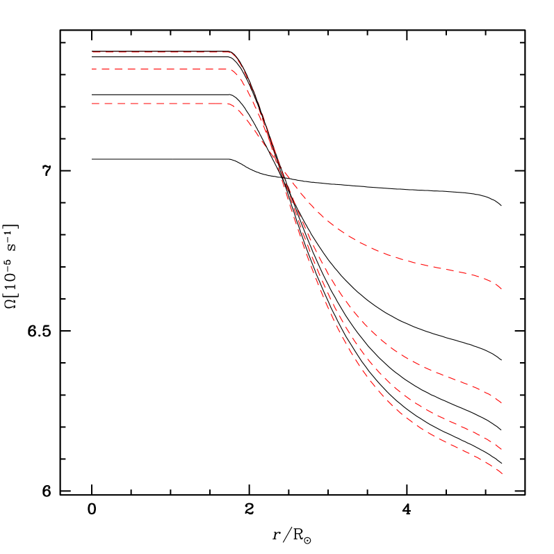
Figure 1: Initial evolution of the angular velocity $\Omega$ as a function of the distance to the center in a 20 M_⊙ star with $v_{\rm ini}$ = 300 km s^-1. Starting from a flat profile, the solutions rapidly converge towards an equilibrium solution. The time interval between two consecutive curves is 19 200 years.

Fig. 1 shows the results for the initial convergence on the zero age main sequence of $\Omega(r)$ in a 20 M_⊙ model with solar composition. The initial model on the zero–age main sequence is supposed to rotate uniformly and with an initial surface velocity $v_{\rm ini}$ of 300 km s^-1. Very short time steps of the order of 1920 yr are taken in the initial calculations for obtaining the internal equilibrium rotation. The results are shown in Fig. 1 for every 10^th model, i.e. with time intervals of 19 200 yr. We see the very fast initial changes of $\Omega(r)$, mainly due to the meridional circulation. The circulation velocity, which is very large, is also positive everywhere at the beginning (cf. Fig. 2). This means that the circulation rises along the polar axis and goes down at the equator, thus bringing angular momentum inwards. As a consequence the angular velocity of the core increases, while that in the envelope goes down. It is important to realize that here these fast changes of the rotation law are not due, as later in the evolution, to core contraction and envelope expansion.

We see that the changes are big at the beginning and then smaller. The profiles of $\Omega(r)$ rapidly converges towards an equilibrium–profile in a time of about 1 to 2% of the MS lifetime $t_{\rm MS}$. This is in agreement with the results for 10 and 30 M_⊙ stars by Denissenkov et al. (Den99 (1999)). As noted by these authors, the timescale for the adjustment of the rotation law, i.e. $t_{\rm circ}\simeq R/U$, is short with respect to the MS lifetime for any significant rotation. Later on during the bulk of MS evolution, the profiles $\Omega(r)$ will evolve more slowly. As emphasized in Sect. 2.6, this timescale $t_{\rm circ}$ is not characteristic for the mixing of chemical elements. We also notice that the degree of differential rotation in the equilibrium profile is rather modest (cf. Zahn, Za92 (1992)).

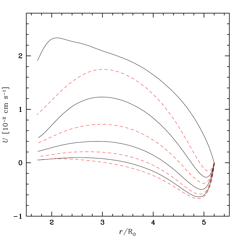
Figure 2: Same as Fig. 1 for $U(r)$ the vertical component of the meridional circulation velocity (cf. Eq. 4). Time proceeds from top to bottom.

Fig. 2 shows the corresponding initial evolution of the vertical component $U(r)$ of the velocity of the meridional circulation in the 20 M_⊙ model. As seen above, initially this velocity is large and positive everywhere, which explains the fast evolution of $\Omega(r)$ in Fig. 1. Then, $U(r)$ decreases and becomes negative in the very external layers. The physical reason for that is the so called Gratton–Öpik term of the form $-\frac{\Omega^{2}}{2\pi G\rho}$ which is contained in the expression of $E_{\Omega}$ in Eq. (12). When the density is very low, as in the outer regions, this negative term becomes important and produces an inverse circulation. This means that the circulation has two big cells, an internal cell rising along the polar axis and an external one descending at the pole. The velocity $U(r)$ also converges towards an equilibrium distribution, characterized by small velocities $U(r)$, a result in agreement with Denissenkov et al. (Den99 (1999)).

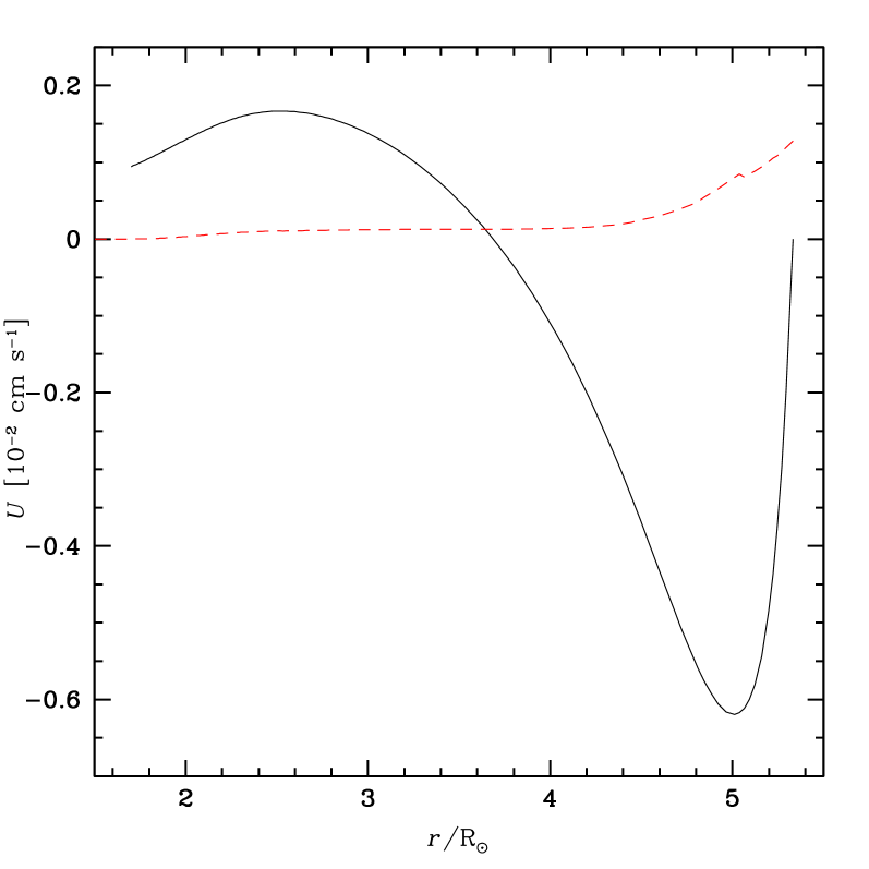
Figure 3: Non–stationary (continuous line) and stationary (broken line) solutions for $U(r)$ the vertical component of the velocity of the meridional circulation (cf. Eq. 4) as a function of the distance to the center in the 20 M_⊙ model at the end of the initial convergence.

It is interesting to compare the stationary solution of $U(r)$ given by Eq. (5) and the non–stationary solution given by Eq. (12). This is done in Fig. 3, where the curve in continuous line corresponds to the asymptotic distribution reached in the non–stationary regime illustrated in Fig. 2. This curve shows positive values of $U(r)$ in the inner regions and negative values in the outer ones. On the contrary, the solution (broken line) obtained in the stationary approximation given by Eq. (5) is always positive. This is a logical consequence of the approximation made: as $\Omega(r)$ decreases outwards, only positive values of $U(r)$ are possible. Said in other words, the outward transport by shears can only be compensated by the inward transport by meridional circulation, i.e. by positive values of $U(r)$.

However, in non–stationary models, this compensation is not achieved since the two curves in Fig. 3 are very different. One concludes that the stationary approximation which has been used in some works (cf. Urpin et al. Urp96 (1996)) is not satisfactory.

The stationary solution can also be viewed as giving a velocity which is the inverse of a velocity which could be associated to the diffusive transport by shears. From the comparison of the two curves in Fig. 3, one thus immediately concludes that the meridional circulation is much more efficient for the transport of the angular momentum than the shear instabilities. The justification for this claim is the following one. In the stationary situation, shear transport and meridional circulation compensate each other and are thus of the same magnitude. The fact that $U(r)$ in the full non–stationary case treatment is much larger than in the stationary case as shown in Fig. 3 implies that the effects of meridional circulation on the transport of angular momentum are much larger than the effects of the shear. This conclusion can also be deduced from the comparison of the timescales for the two processes. In general one has that $t_{\rm circ}=\frac{R}{U}<t_{\rm shear}=\frac{R^{2}}{D_{\rm shear}}$. For the chemical elements, the transport by the shear instabilities is more efficient than the transport by the meridional circulation as discussed in Sect. 2.6 where we have seen that $D_{\rm eff}$ is reduced by horizontal turbulence.

4.2 Internal evolution of $\Omega(r)$

The evolution of $\Omega(r)$ during the MS evolution of a 20 M_⊙ star is shown in Fig. 4. We notice that initially (i.e. for high values of the central H–content $X_{\rm{c}}$), the degree of differential rotation is small, then, it grows during the evolution. The ratio between the central and surface value of $\Omega$ remains however small during the MS evolution. The rotation rate does not vary by more than about a factor two throughout the star. Although this degree of differential rotation is not large, it plays an essential role in the shear effects and the related transports of angular momentum and of chemical elements. The same remark also applies to the effects of differential rotation on the transport by meridional circulation, since $U(r)$ critically depends on the derivatives of $\Omega$ in the star (cf. Zahn 1992; Maeder & Zahn 1998).

We notice a general decrease of $\Omega(r)$, even in the convective core which is contracting. The main reason is mass loss at the stellar surface, which removes a substantial fraction of the total angular momentum. This makes $\Omega(r)$ to decrease with time everywhere, because of the internal transport mechanisms, which ensure some coupling of rotation. The same behaviour was obtained by Langer (1998) in the case of rigid rotation (i.e. in the case of maximum coupling). In the present models, shear transports the angular momentum outwards, which reduces the core rotation, while circulation makes an inward transport in the deep interior and an outwards transport in the external region. This is responsible for the progressive flattening of the curves above $r=4R_{\odot}$ in Fig. 4.

Figure 4: Evolution of the angular velocity $\Omega$ as a function of the distance to the center in a 20 M_⊙ star with $v_{\rm ini}$ = 300 km s^-1. $X_{c}$ is the hydrogen mass fraction at the center. The dotted line shows the profile when the He–core contracts at the end of the H–burning phase.

From the end of the MS evolution onwards, i.e. when $X_{c}\leq 0.05$, central contraction becomes faster and starts dominating the evolution of the angular momentum in the center. The central $\Omega$ grows quickly (cf. dotted curve in Fig. 4) and this will in principle continue in the further evolutionary phases until core collapse. The evolution of the angular momentum after the H–burning phase ($X_{c}=0$) is mainly dominated by the local conservation of the angular momentum, since the secular transport mechanisms have little time to operate. This is the assumption we are making in the present models. During these phases, the chemical elements continue to be rotationally mixed in the radiative layers mainly through the effect of the shear. In the further evolutionary phases, the strong central contraction will lead to very large central rotation, unless some other processes as fast dynamical instabilities or magnetic braking occur in these stages.

Figure 5: Same as Fig. 4 for $U(r)$.

The evolution of $U(r)$ during MS evolution is shown in Fig. 5. The outer zone with inverse circulation progressively deepens in radius during MS evolution due to the Gratton–Öpik term, because a growing part of the outer layers has lower densities. Also, we notice that the velocities $U(r)$ are small in general (cf. Urpin et al. Urp96 (1996)) and tests have shown us that, contrary to the classical result of the Eddington–Sweet circulation (cf. Mestel 1965), $U(r)$ depends rather little on the initial rotation.

The deepening of the inverse circulation has the consequence that the stationary and non–stationary solutions differ more and more as the evolution proceeds, since as said above no inverse circulation is predicted by the stationary solution. Thus we conclude that the stationary solutions are much too simplified. Also, in Fig. 5, we see that the values of $U(r)$ become more negative in the outer layers for the model at the end of the MS phase, when central contraction occurs. Again, this effect is due to the Gratton–Öpik term. The results of Fig. 5 also shows that the application of a diffusive treatment to meridional circulation transport is unappropriate. Paradoxically, the problem is less serious in regions which exhibit an inverse circulation, since there the signs of the effects are at least the same in the two treatments (however even there the equations for advection and diffusion are different).

Figure 6: Internal values of $K$ the thermal diffusivity, $D_{\rm h}$ the coefficient of horizontal turbulence, $D_{\rm shear}$ the shear diffusion coefficient, $D_{\rm eff}$ the effective diffusivity (cf. Eq. 9) and $\nu$ the total viscosity (radiative + molecular) in the radiative envelope of a 20 M_⊙ star with an initial $v_{\rm ini}$ = 300 km s^-1. The lagrangian mass coordinate is given on the upper scale. Here, the hydrogen mass fraction at the center $X_{c}=0.20$.

The various diffusion coefficients inside a 20 M_⊙ star are shown in Fig. 6, when the hydrogen mass fraction $X_{c}$ at the center is equal to 0.20. We notice that in general $K>D_{h}>D_{\rm shear}>D_{\rm eff}>\nu$. Following the thermal diffusivity $K$, the coefficient of horizontal diffusion $D_{h}$ is the second largest one, this is consistent and necessary for the validity of the assumption of shellular rotation (Zahn, Za92 (1992)). Since we have $D_{\rm{shear}}=2K\Gamma$ according to Eq. (18), Fig. 6 shows that $\Gamma$ is typically of the order of 10^-3 to 10^-4. The coefficient $D_{\rm{eff}}$, expressing the transport of the chemical elements by the meridional circulation with account of the reduction by the horizontal turbulence, is only slightly smaller (by a factor of about 3) than $D_{\rm{shear}}$ in the interior. One must be careful that $D_{\rm{eff}}$ concerns only the tranport of the elements and not that of angular momentum, for which meridional circulation is the largest effect. Fig. 6 also shows the values of the total viscosity $\nu$, and we notice that consistently the Prandtl number $\nu/K$ is of the order of 10^-5 to 10^-6.

5 HR diagram, lifetimes and age estimates

5.1 The Main–Sequence evolution

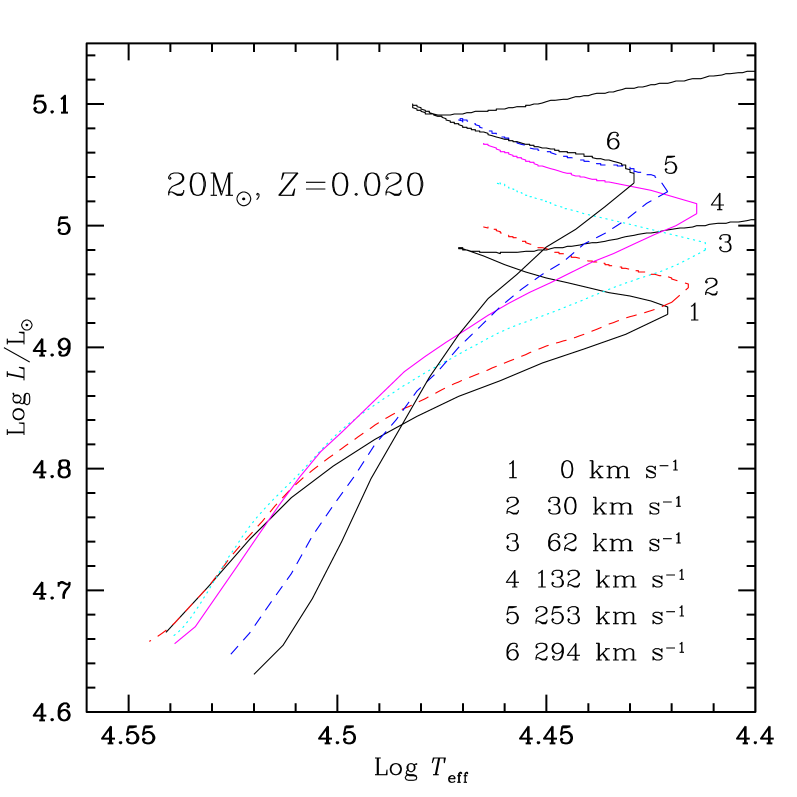
Figure 7: Evolutionary tracks for rotating 20 M_⊙ models with different initial velocities. The mean equatorial velocities $\overline{v}$ during the MS are indicated. The corresponding initial velocities can be seen in Table 2.

Evolutionary tracks of 20 M_⊙ models at solar metallicity for different initial velocities are plotted on Fig. 7. The $T_{\rm eff}$ for a rotating star has been defined in Sect. 2.3. On and near the ZAMS, rotation produces a small shift of the tracks towards lower luminosities and $T_{\rm eff}$. This effect is due to both atmospheric distorsions and to the lowering of the effective gravity (see e.g. Kippenhahn and Thomas KippTh70 (1970); Maeder and Peytremann MP70 (1970); Collins and Sonneborn co77 (1977)). At this stage the star is still nearly homogeneous. When evolution proceeds, the tracks with rotation become more luminous than for no rotation. This results from essentially two effects. On one side, rotational mixing brings fresh H–fuel into the convective core, slowing down its decrease in mass during the MS. For a given value of the central H–content, the mass of the convective core in the rotating model is therefore larger than in the non–rotating one and thus the stellar luminosity is higher (Maeder ma87 (1987); Talon et al. Ta97 (1997); Heger et al. He00 (2000)). As a numerical example, in the $v_{\rm ini}=$ 300 km s^-1 models the He–cores at the end of the MS are about 20% more massive than in their non–rotating counterparts. This is equal to the increase obtained by a moderate overshooting (see Sect. 3). On the other side, rotational mixing transports helium and other H–burning products (essentially nitrogen) into the radiative envelope. The He–enrichment lowers the opacity. This contributes to the enhancement of the stellar luminosity and favours a blueward track. Indeed, in Fig. 7, one sees that when the mean velocity on the MS becomes larger than about 130 km s^-1, the $T_{\rm eff}$ at the end of the MS increases when rotation increases.

For sufficiently low velocities, rotation acts as a small overshoot, extending the MS tracks towards lower $T_{\rm eff}$. This results from the fact that, at sufficiently low rotation, the effect of rotation on the convective core mass overcomes the effect of helium diffusion in the envelope. Indeed, for small rotation, the time required for helium mixing in the whole radiative envelope is very long, while hydrogen just needs to diffuse through a small amount of mass to reach the convective core.

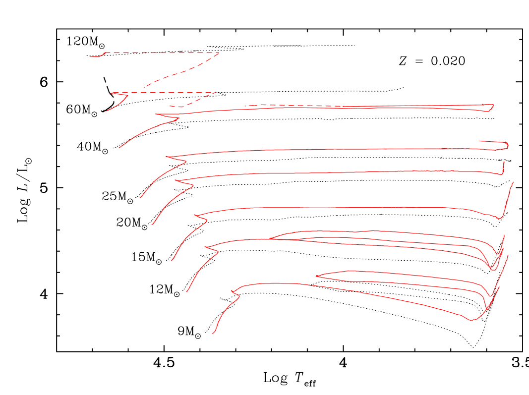
Figure 8: Evolutionary tracks for non–rotating (dotted lines) and rotating (continuous lines) models with solar metallicity. The rotating models have an initial velocity $v_{\rm ini}$ of 300 km s^-1. For purpose of clarity, only the first part of the tracks for the most massive stars (M $\geq 40$ M_⊙) is shown. Portions of the evolution during the W–R phase for the rotating massive stars are indicated by short–dashed lines. The long–dashed track for the 60 M_⊙ model corresponds to a very fast rotating star ($v_{\rm ini}$ $\sim 400$ km s^-1), which follows a nearly homogeneous evolution. Only the beginning of its evolution is shown.

Since not all the stars have the same initial rotational velocity, one expects a dispersion of the luminosities at the end of the MS. For the 20 M_⊙ models shown on Fig. 7 one sees a difference of $\sim 0.3$ in $M_{\rm bol}$ between the luminosities of the low and fast rotators at the end of the MS. Rotation induces also a scatter of the effective temperatures at the end of the MS. In reality, the dispersion results from both different initial velocities and also, for a given initial velocity, from different angles between the axis of rotation and the line of sight. Indeed due to the von Zeipel theorem (vZ24 (1924)) the star appears bluer seen pole–on than equator–on. When integrated over the visible part of the star, the effects due to orientation can reach a few tenths of a magnitude in luminosity and a few hundredths in $\log T_{\rm eff}$ (cf. Maeder and Peytreman 1970).

Figure 8 shows the evolutionary tracks of non–rotating and rotating stellar models for initial masses between 9 and 120 M_⊙. For the rotating stellar models, the initial velocity is $v_{\rm ini}$ = 300 km s^-1. There is little difference between tracks with $v_{\rm ini}$ = 200 or 300 km s^-1 (see also Talon et al. Ta97 (1997)). If the effects behaved like $v_{\rm ini}^{2}$, there would be larger differences. The present saturation effect occurs because outward transport of angular momentum by shears are larger when rotation is larger, also a larger rotation produces more mass loss, which makes a larger reduction of rotation during the evolution. Let us note however that for some surface abundance ratios as N/C or N/O (see Table 1), the increase from $v_{\rm ini}$ = 200 to 300 km s^-1 produces significant changes. Thus, the similarity of the evolutionary tracks does not necessarily imply the similarity of the surface abundances for these elements.

Rotation reduces the MS width in the high mass range (M $\mathbin{\;\raise 1.0pt\hbox{$<$}\kern-8.0pt\lower 3.0pt\hbox{$\sim$}\;}40$ M_⊙). Let us recall that when the mass increases, the ratio of the diffusion timescale for the chemical elements to the MS lifetime decreases (Maeder ma98 (1998)). As a consequence, starting with the same $v_{\rm ini}$ on the ZAMS, massive stars will be more mixed than low mass stars at an identical stage of their evolution. This reduces the MS width since greater chemical homogeneity makes the star bluer. Moreover, due to both rotational mixing and mass loss, their surface will be rapidly enriched in H–burning products. These stars will therefore enter the Wolf–Rayet phase while they are still burning their hydrogen in their core. This again reduces the MS width. For initial masses between 9 and 25 M_⊙, the MS shape is not much changed by rotation at least for $v_{\rm ini}\leq 300$ km s^-1.

5.2 The post–Main-Sequence evolution

The post–MS evolution of the most massive stars (M $\geq 40$ M_⊙) which become W–R stars will be discussed in a forthcoming paper. We shall just mention one point of general interest here: for low or moderate rotation, the convective core shrinks as usual during MS evolution, while for high masses ($M\mathbin{\;\raise 1.0pt\hbox{$>$}\kern-8.0pt\lower 3.0pt\hbox{$\sim$}\;}40$ M_⊙) and large initial rotations ($\frac{\Omega}{\Omega_{\rm crit}}\geq 0.5$), the convective core grows in mass during evolution. This latter situation occurs in the fast rotating 60 M_⊙ model shown on Fig. 8. These behaviours, i.e. reduction or growth of the core, determine whether the star will follow respectively the usual redwards MS tracks in the HR diagram, or whether it will bifurcate to the blue (cf. Maeder ma87 (1987); Langer la92 (1992)) towards the classical tracks of homogeneous evolution (Schwarzschild sc58 (1958)) and likely produce W–R stars.

The stars with initial masses between 15 and 25 M_⊙ become red supergiants (RSG). Rotation does not change qualitatively this behaviour but accelerates the redwards evolution, especially for the 15 and 20 M_⊙ models. As a numerical example, for an initial $v_{\rm ini}$ = 300 km s^-1, the model stars burn all their helium as red supergiants at $T_{\rm eff}$ below 4000 K, while the non–rotating models spend a significant part of the He–burning phase in the blue part of the HR diagram: for the non–rotating 15 and 20 M_⊙ models, respectively 25 and 20% of the total He–burning lifetime is spent at $\log T_{\rm eff}\geq 4.0$. The behaviour of the rotating models results mainly from the enhancement of the mass loss rates. This effect prevents the formation of a big intermediate convective zone and therefore favours a rapid evolution toward the RSG phase (Stothers and Chin st79 (1979); Maeder ma81 (1981)). Let us note that the dispersion of the initial rotational velocities produces a mixing of the above behaviours.

Very interestingly, for the 12 M_⊙ model a blue loop appears when rotation is included. This results from the higher luminosity of the rotating model. The higher luminosity implies that the outer envelope is more extended, and is thus characterized by lower temperatures and higher opacities at a given mass coordinate. As a consequence, in the rotating model during the first dredge–up, the outer convective zone proceeds much more deeply in mass than in the non–rotating star. Typically in the non–rotating model the minimum mass coordinate reached by the outer convective zone is 6.6 M_⊙ while in the rotating model it is 2.6 M_⊙. This prevents temporarily the extension in mass of the He–core and enables the apparition of a blue loop. Indeed the lower the mass of the He–core is, the lower its gravitational potential. According to Lauterborn et al. (la71 (1971), see also the discussion in Maeder and Meynet ma89 (1989)), a blue loop appears when the gravitational potential of the core $\Phi_{c}$ is inferior to a critical potential $\Phi_{\rm crit}$ depending only on the actual mass of the star which is about the same for the rotating and non–rotating model. This explains the appearance of a blue loop in the 12 M_⊙ rotating model. For the 9 M_⊙ model, the minimum mass coordinate reached by the outer convective zone is not much affected by rotation and the models with and without rotation present very similar blue loops.

Table 1: Properties of the stellar models at the end of the H–burning phase, at the blue supergiant (BSG) or LBV stage (see text) and at the end of the He–burning phase. The masses are in solar mass, the velocities in km s^-1, the lifetimes in million years and the abundances in mass fraction.

M	$v_{\rm ini}$	$\overline{v}$	End of H–burning						BSG or LBV				End of He–burning
			$t_{H}$	M	$v$	Ys	N/C	N/O	$v$	Ys	N/C	N/O	$t_{He}$	M	$v$	Ys	N/C	N/O
120	0	0	2.557	76.070	0	0.55	57.8	1.48	0	0.66	55.6	24.2	0.326	58.024	0	0.85	47.4	45.1
	300	163	2.890	57.901	65	0.89	49.3	45.4	65	0.91	48.5	46.8	0.357	16.201	27	0.22	0	0
60	0	0	3.366	47.517	0	0.30	0.26	0.12	0	0.46	10.3	2.26	0.394	14.960	0	0.23	0	0
	200	107	3.922	40.989	29	0.59	18.6	5.55
	300	168	4.128	25.066	29	0.90	49.6	30.2	49	0.93	49.6	34.8	0.423	11.697	46	0.39	0	0
40	0	0	4.155	34.761	0	0.30	0.25	0.12	0	0.30	0.25	0.12	0.473	12.565	0	0.98	41.4	47.4
	200	114	4.936	31.871	38	0.43	4.29	1.49
	300	172	5.105	30.898	104	0.47	5.33	1.85	15	0.48	5.39	1.87	0.462	11.872	119	0.35	0	0
25	0	0	5.928	23.213	0	0.30	0.25	0.12	0	0.30	0.25	0.12	0.737	18.912	0	0.44	3.95	1.22
	200	125	7.114	22.089	77	0.34	1.40	0.52
	300	183	7.442	21.640	154	0.37	2.07	0.72	90	0.38	2.15	0.75	0.718	11.657	0.4	0.65	36.4	3.40
20	0	0	7.350	19.019	0	0.30	0.25	0.12	0	0.30	0.25	0.12	1.032	17.043	0	0.38	2.02	0.70
	200	132	8.901	18.324	94	0.32	1.01	0.38
	300	197	9.309	18.020	167	0.35	1.77	0.58	34	0.35	1.80	0.59	0.871	14.605	0.3	0.48	5.70	1.40
15	0	0	10.214	14.631	0	0.30	0.25	0.12	0	0.30	0.25	0.12	1.506	13.728	0	0.34	1.30	0.45
	200	145	12.316	14.365	142	0.31	0.69	0.26
	300	209	12.917	14.260	226	0.32	1.36	0.43	60	0.33	1.43	0.45	1.482	12.589	31	0.44	4.69	1.06
12	0	0	13.929	11.926	0	0.30	0.25	0.12	0	0.30	0.25	0.12	2.368	11.100	0	0.32	1.07	0.36
	200	150	16.069	11.867	141	0.30	0.60	0.23
	300	217	16.797	11.828	242	0.31	1.07	0.34	139	0.41	4.37	0.91	2.503	10.873	1.2	0.41	4.42	0.91
9	0	0	22.054	8.991	0	0.30	0.25	0.12	0	0.32	1.32	0.42	3.728	8.875	0	0.32	1.32	0.42
	200	153	25.862	8.982	158	0.30	0.41	0.17
	300	235	26.737	8.977	266	0.31	0.86	0.29	98	0.37	3.59	0.73	3.997	8.770	2.4	0.37	3.59	0.73

5.3 Masses and mass–luminosity relations

When rotation increases, the actual masses at the end of both the MS and the He–burning phases become smaller (cf. Tables 1 and 2). Typically the quantity of mass lost by stellar winds during the MS is enhanced by 60–100% in rotating models with $v_{\rm ini}$ = 200 and 300 km s^-1 respectively. For stars which do not go through a Wolf–Rayet phase, the increase is due mainly to the direct effect of rotation on the mass loss rates (in the present models through the formula proposed by Friend and Abbott Fr86 (1986)) and to the higher luminosities reached by the tracks computed with rotation. The fact that rotation increases the lifetimes also contributes to produce smaller final masses. For the most massive stars (M $\geq 60$ M_⊙), the present rotating models enter the Wolf–Rayet phase already during the H–burning phase (see also Maeder 1987; Fliegner & Langer 1995; Meynet 1999, 2000b). This reduces significantly the mass at the end of the H–burning phase.

As indicated in Sect. 5.1, the initial distribution of the rotational velocities implies a dispersion of the luminosities at the end of the MS. This effect introduces a significant scatter in the mass–luminosity relation (Langer 1992; Meynet me98 (1998)), in the sense that fast rotators are overluminous with respect to their actual masses. This is especially true in the high mass star range in which the luminosity versus mass relation flattens. This may explain some of the discrepancies between the evolutionary masses and the direct mass estimates in some binaries (Penny et al. pe99 (1999)).

Let us end this section by saying a few words about the mass discrepancy problem (see e.g. Herrero et al. He00 (2000)). For some stars, the evolutionary masses (i.e. determined from the theoretical evolutionary tracks) are greater that the spectroscopically determined masses. Interestingly, according to Herrero et al. (He20 (2000)), only the low gravity objects present (if any) a mass discrepancy. Even if most of the problem has collapsed and was shown to be a result of the proximity of O–stars to the Eddington limit (Lamers and Leitherer la93 (1993); Herrero et al. He99 (1999)) and of the large effect of metal line blanketing not usually accounted for in the atmosphere models of massive stars (Lanz et al. la96 (1996)), some discrepancy seems to be still present. The remaining mass discrepancy may arise, in part, from the use of non–rotating models for determining the evolutionary masses. High rotation produces larger He–cores and He–rich envelopes, all that implies overluminous stars with lower gravity as evolution proceeds. This can occur even for the slow rotating objects because they could have had a sufficiently high initial rotational velocity. The observation that the mass discrepancies are found only for low gravity objects may reflect the fact that rotation implies more and more important changes in the $\log g_{\rm eff}$ versus $\log T_{\rm eff}$ plane when evolution proceeds. Indeed, looking at Fig. 16 below one sees that at high gravity (i.e. at an early evolutionary stage), one does not expect any mass difference when using rotating or non–rotating tracks. In contrast, the mass difference between the rotating and the non–rotating tracks become more and more important in the high mass star range and for the low values of $\log g_{\rm eff}$. The rotating 40 M_⊙ track crosses the non–rotating 60 M_⊙ model on Fig. 16 indicating that differences of $\sim$30% in mass are quite possible.

For the fast rotating objects, a part of the mass discrepancy may also be due to a possible underestimate of the gravity (see Sect. 7.1). Indeed, an underestimate of the gravity would also imply an underestimate of the spectroscopically determined masses (Herrero et al. 2000).

5.4 Lifetimes and isochrones

Table 1 presents some properties of the models. Column 1 and 2 give the initial mass and the initial velocity $v_{\rm ini}$ respectively. The mean equatorial rotational velocity $\overline{v}$ during the MS phase is indicated in column 3. This quantity is defined by

$$\overline{v}=1/t_{H}\int_{0}^{t_{H}}v(t)dt,$$

where $t_{H}$ is the duration of the H–burning phase given in column 4, except for those stars which enter the Wolf–Rayet phase while still burning their hydrogen in their core, i.e. for the rotating 60 and 120 M_⊙ models, for which $t_{H}$ has been replaced by the duration of the O–type star phase. The H–burning lifetimes $t_{H}$, the masses M, the equatorial velocities $v$, the helium surface abundance $Y_{s}$ and the surface ratios (in mass) N/C and N/O at the end of the H–burning phase are given in columns 4 to 9. The columns 10 to 13 present some properties of the models when the star is a blue supergiant (BSG) or an LBV star. For stellar models with M$\leq 40$ M_⊙, the “BSG stage” in Table 1 corresponds either to the stage when $\log T_{\rm eff}=4.0$ during the first crossing of the Hertzsprung–Russel diagram or to the bluest point on the blue loop if any for M$\leq 12$ M_⊙. For non–rotating stellar models with M $\geq 60$ M_⊙, the “LBV stage” corresponds to the point when the star has lost half of the matter ejected by the stellar winds between the end of the MS and the entrance into the W–R phase. In the case of rotating models, the “LBV stage” corresponds to the period during which the surface velocity becomes critical and huge mass loss rates ensue. Again, here we choose a model in the middle of this phase. The columns 14 to 19 present some characteristics of the stellar models at the end of the He–burning phase and $t_{He}$ is the He–burning lifetime. In Table 2 some properties of 20 M_⊙ models at the end of the MS are indicated, $v_{\rm ini}$ and $\overline{v}$ have the same meaning as above.

Table 2: Properties of 20 M_⊙ models at the end of the MS for different initial velocities. The velocities are in km s^-1, the lifetimes in million years, the masses in solar mass and the abundances in mass fraction.

$v_{\rm ini}$	$\overline{v}$	$t_{H}$	M	$v$	Ys	N/C	N/O
0	0	7.350	19.019	0	0.30	0.25	0.12
50	30	7.720	18.896	18	0.30	0.27	0.12
100	62	8.292	18.681	46	0.30	0.45	0.19
200	132	8.901	18.324	94	0.32	1.01	0.38
300	197	9.309	18.020	167	0.35	1.77	0.58
400	253	9.745	17.646	217	0.37	2.54	0.76
500	294	10.275	17.181	213	0.40	3.65	0.99
580	304	10.324	17.148	214	0.39	3.75	1.00

From Table 1 one sees that for $Z=0.020$ the lifetimes are increased by about 20–30% when the mean rotational velocity on the MS increases from 0 to $\sim$200 km s^-1. This modest increase is explained by the fact that even if there is more fuel available in the core, the luminosity is also increased. From the data presented in Table 2, one can deduce a nearly linear relation between the relative enhancement of the MS lifetime, $\Delta t_{\rm H}$ and $\overline{v}$, where

$$\Delta t_{\rm H}(\overline{v})=[t_{\rm H}(\overline{v})-t_{\rm H}(0)]/t_{\rm H}(0).$$

One obtains,

$${\Delta t_{\rm H}(\overline{v})\over t_{\rm H}(0)}=0.0013\cdot\overline{v},$$

where $\overline{v}$ is in km s^-1. This relation reproduces the values of $\Delta t_{H}(\overline{v})/t_{H}(0)$ from table 2 with an accuracy better than 5%. It also applies with the same accuracy to the values listed in Table 1 for the masses between 15 and 40 M_⊙. The He–burning lifetimes are less affected by rotation than the MS lifetimes. The changes are less than 10%. The ratios $t_{He}/t_{H}$ of the He to H–burning lifetimes are only slightly decreased by rotation and remain around 10–15%.

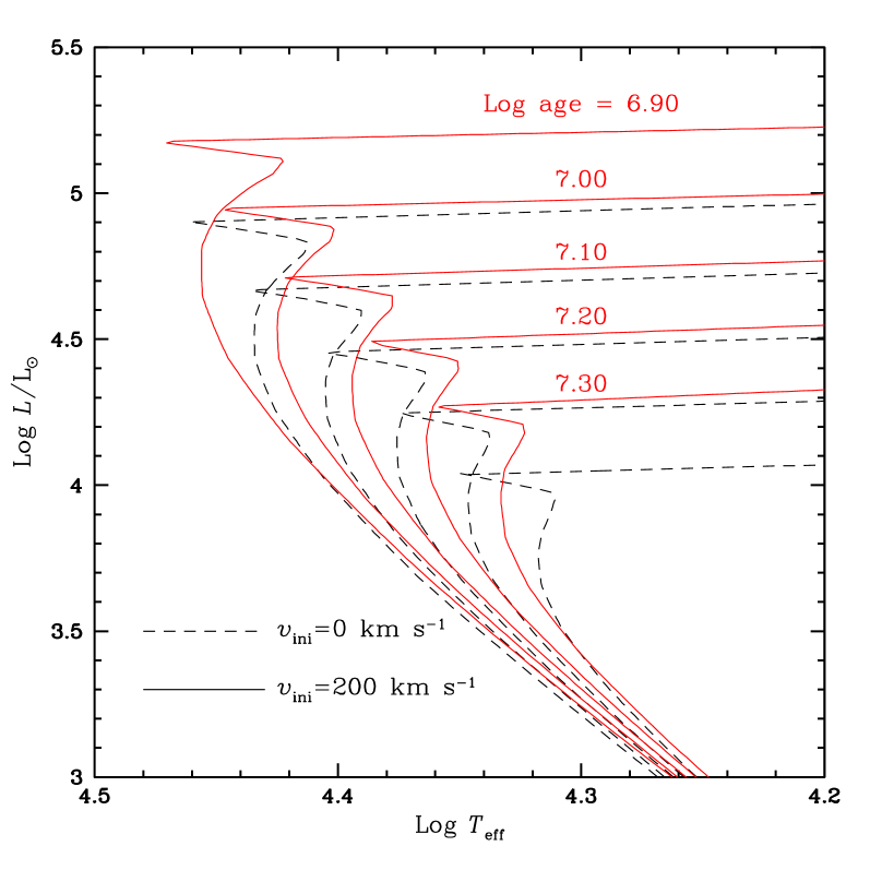
Figure 9: Isochrones computed from stellar evolutionary tracks for the solar metallicity. The dashed and continuous lines correspond to the case of non–rotating and rotating stellar models respectively. In this last case, models have an initial velocity $v_{\rm ini}$ of 200 km s^-1. The logarithms of the ages (in years) label the isochrones computed from the models with rotation.

On Fig. 9 isochrones for ages between about 8 and 20 10⁶ yr, computed from non–rotating and rotating stellar models are presented. The “rotating” isochrones are computed from the models with an initial rotational velocity $v_{\rm ini}$ of 200 km s^-1 on the ZAMS.

At a given age, the upper part of the “rotating” isochrones are bluer and more luminous. Typically, for an age equal to about $20\cdot 10^{6}$ years ($\log$ age =7.3) the reddest point on the MS is shifted by 0.015 dex in $\log T_{\rm eff}$ and by - 0.6 in $M_{\rm bol}$ when rotation is taken into account. An isochrone with rotation is almost identical to an isochrone without rotation with log age smaller by 0.1 dex. This has for consequence that rotation slightly increases the age associated to a given cluster. From Fig. 9, one sees that the “rotating” isochrone for an age equal to $20\cdot 10^{6}$ years has the same luminosity at the turn–off than the “non-rotating” isochrone for an age equal to $16\cdot 10^{6}$ years. Thus rotation increases the age estimate by about 25%. We may wonder whether this effect explains the age difference between the estimates based on the upper MS and the estimates based on the lithium content of the very low mass stars (see e.g. Martin et al. 1998; Barrado y Navascués et al. 1999). One must also account for the dispersion of rotational velocities and possibly of the orientation angles. These two effects introduce some dispersion in the way stars are distributed in the HR diagram and thus affect the interpretation of the clusters’ observed sequences (cf. Maeder ma71 (1971)).

If a bluewards track occurs, as for very massive stars with fast rotation, the larger core and mixing lead to much longer lifetimes in the H–burning phase. In this case, the fitting of time–lines becomes hazardous.

6 Evolution of the rotational velocities

6.1 Model results for stars with a large mass loss

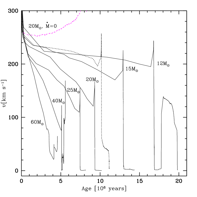
Figure 10: Evolution of the surface equatorial velocity as a function of time for stars of different initial masses with $v_{\rm ini}$ = 300 km s^-1. The continuous lines refer to solar metallicity models, the dotted line corresponds to a 20 M_⊙ star with $Z$ = 0.004. The dashed line corresponds to a 20 M_⊙ star without mass loss.

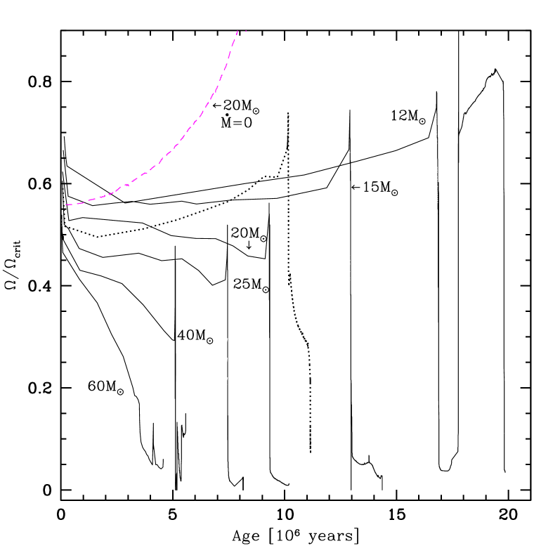
Figure 11: Same as Fig. 10 for the ratio $\Omega/\Omega_{\rm crit}$ of the angular velocity to the break–up velocity at the stellar surface.

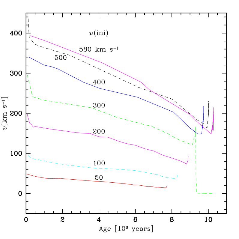
Figure 12: Evolution of the surface equatorial velocity as a function of time for 20 M_⊙ stars with different initial velocities.

Figs. 10 and 11 show the evolution of $v$ and of $\frac{\Omega}{\Omega_{\rm{crit}}}$ as a function of the age for the present models. Firstly, we notice that for models without mass loss, as shown for the 20 M_⊙ with $\dot{M}$ = 0, $v$ and $\frac{\Omega}{\Omega_{\rm{crit}}}$ go up fastly so that the critical velocity would be reached near the end of the MS phase. The current model of 20 M_⊙ with mass loss show a significant decrease of $v$, while the critical ratio remains almost constant during most of the MS phase. Figs. 10 and 11 show how fastly rotation decreases at the surface of the most massive stars, which lose a lot of mass. Consistently we see that the reduction of the surface rotation is much larger for the more massive stars. This is of course a consequence of the removal of large amounts of angular momentum by the stellar winds. The effect is amplified by the increase of the mass loss in fast rotators (Eq. 2). We see that the decrease of $\frac{\Omega}{\Omega_{\rm{crit}}}$ is so strong that it will prevent a massive star to reach the critical velocity near the end of the MS phase. If the star makes extended excursions in the HR diagram at the end of the MS like is the case for the 60 M_⊙ model, then it may reach the critical velocity. The specific case of stars close to the $\Omega$–limit will be examined in a future study, since this requires some further theoretical developments.

Let us mention here that the present results differ from those obtained by Sackmann and Anand (Sa70 (1970)) and Langer (La97 (1997), La98 (1998)). Indeed, these authors find that the star reaches the break–up limit during the MS phase. As an example, in a 60 M_⊙ star, even a model with an initial $v_{\rm{ini}}$ of 100 km s^-1 reaches the break–up limit near the end of the MS–phase (Langer 1998). This result leads Langer to conclude that most massive stars may reach the break–up limit or the so–called $\Omega$–limit during their MS evolution. Let us however emphasize here that such a conclusion is based on a particular definition of $v_{\rm crit}$ still subject to discussion (see Sect. 2.4), on the assumption of solid body rotation, and on models not accounting for the effects of rotationnally induced mixing. We see here that modifying these hypothesis (and also using other prescriptions for the mass loss rates) lead to very different results. One of the first step to clarify the situation is to determine which expression for $v_{\rm crit}$ (cf. Glatzel 1998; Langer 1998) is the correct one and how rotation affects the mass loss rates. These developments, now in progress, will be particularly needed for the study of the evolution of the most massive stars, like a 120 M_⊙ model, which have a high value of the Eddington factor. Also this is important for the formation and evolution of W–R stars, which will be studied in a further work.

Figure 13: Evolution of the equatorial surface velocities along the evolutionary tracks in the HR diagram starting from $v_{\rm ini}$ = 300 km s^-1. For purpose of clarity, only the first part of the 40 M_⊙ track is shown.

Fig. 12 shows the evolution of $v$ with age for models of a 20 M_⊙ star with different initial velocities $v_{\rm ini}$ from 50 to 580 km s^-1. We see that the decrease in the surface $v$ is larger for larger initial rotation. This is a consequence of the larger mass loss rates in fast rotators. We notice some convergence (cf. Langer 1998) of the curves for the large initial $v_{\rm{ini}}$. This convergence would be more pronounced and affect the models with lower $v_{\rm ini}$ if the dependence of $\dot{M}$ vs $v$ would be stronger than given by Eq. (2). This certainly reduces the scatter of $v$ near the end of the MS phase, but does not produce a full convergence.

6.2 Results for stars with lower mass loss

The models of 12 and 15 M_⊙ show curves in Figs. 10 and 11 with little reduction of $v$, while there are slight increases of the critical ratio $\frac{\Omega}{\Omega_{\rm{crit}}}$ during MS evolution. A peak is reached during the overall contraction phase at the end of the MS phase. Then, $v$ and the critical ratio go down as the star moves to the red supergiant phase. During such a fast evolution, we may say that the rotation evolves almost like the case of simplified models, where the angular momentum is conserved locally. The large growth of the radius just implies a decrease of $v$ and of $\frac{\Omega}{\Omega_{\rm{crit}}}$. Later during the blue loops, where the Cepheid instability strip is crossed, the rotation velocity becomes very large again and could easily become close to critical. This behaviour, also found by Heger & Langer (1998), results from the stellar contraction which concentrates a large fraction of the angular momentum of the star (previously contained in the extended convective envelope of the RSG) in the outer few hundredths of a solar mass. This result suggests that rotation may also somehow influence the Cepheid properties, in addition to the increase of stellar luminosity discussed above.

Amazingly, we notice that the stars with initially low mass loss during the MS phase, like for stars with M $\leq 12$ M_⊙, have more chance to reach the break–up velocities and thus huge mass loss than the more massive stars which lose a lot of mass on the MS. It is somehow surprising that little mass loss during the MS may favour large mass loss rates at the end of the MS phase. This may explain why stars close to break–up, like the Be stars, do not form among the O–type stars, but mainly among the B–type stars, where we see that the ratio $\frac{\Omega}{\Omega_{\rm{crit}}}$ may increase during the MS phase. Another related observation is the fact that the relative number of Be–stars with respect to B–type stars is much higher in the LMC and SMC than in the Galaxy (cf. Maeder et al. MGM99 (1999)). In the LMC and SMC, due to the lower metallicity, the average mass loss rates are lower and thus these stars may keep higher rotation in general and thus form more Be stars. This explanation does not exclude differences in the distribution of $v_{\rm{ini}}$ as well.

6.3 The rotational velocities in the HR diagram

The evolution of $v$ in the HR diagram is shown in Fig. 13. Starting with models having a velocity of 300 km s^-1 on the zero–age main sequence, we give some lines of constant $v$ over the HR diagram. On the MS, we notice in particular that the decrease is much faster for the most massive stars than for stars with M $\leq$ 15 M_⊙. This difference remains also present in the domain of B–supergiants. During the crossing of the HR diagram, the rotational velocities decrease fastly, to become very small, i.e. of the order of a few km s^-1, in the red supergiant phase.

It is beyond the scope of this paper to make detailed comparisons of the evolution of the distribution of the velocities over the HR diagram, however, we may notice a few points. The fact that the average $\overline{v}$ is lower for O–type stars than for the early B–type stars (Slettebak, Sl70 (1970)) may be the consequence of the higher losses of mass and angular momentum in the most massive stars. Also, we remark that the increase of $\overline{v}$ from O–stars to B–stars is larger for the stars of luminosity class IV than for class V (Fukuda, Fu82 (1982)). This is consistent with our models, which show (cf. Fig. 13) that the differences of $\overline{v}$ beween O– and B–type stars are much larger at the end of the MS phase. Another fact in the observed data is the strong decrease of $\overline{v}$ for the massive supergiants of OB–types. This is predicted by all stellar models (cf. also Langer La98 (1998)) due to the growth of the stellar radii. Further detailed comparisons may perhaps provide some new tests and constraints.

7 Evolution of the surface abundances

Figure 14: Evolution of the N/C ratios (in mass) at the surface of rotating models for $v_{\rm ini}$ = 300 km s^-1. Dotted lines joining evolutionary stages with the same value of the N/C ratio are superposed on the MS evolutionary tracks. Values of the N/C ratios are indicated at some points during the post–MS phases. The numbers indicated in parentheses correspond to the values of the N/C ratio at the surface of the non–rotating models at the end of the He–burning phase. The initial ratio (N/C)₀ is equal to 0.25. For purpose of clarity, only the first part of the 40 M_⊙ track is shown.

The chemical abundances offer a very powerful test of internal evolution and they give strong evidences in favour of some additional mixing processes in massive stars. A review of the observations may be found in Maeder and Meynet (2000). Here we shall concentrate on the discussion of the theoretical results and we shall compare them with some recent observations.

The most striking feature appearing in Tables 1 and 2 as well as on Fig. 14 is the change of surface abundances in rotating stellar models (cf. Langer 1992). The He–, N–enrichments and the related C– and O–depletions at the surface already occur on the MS. The more massive the star is, the more pronounced are the enrichments, supporting the expectation that mixing becomes more and more efficient when the mass increases (Maeder ma98 (1998)). The same is true when the initial rotational velocity increases. During the crossing of the Hertzsprung–Russel diagram, the evolution is sufficiently short for not allowing any important change of the surface abundances (see Fig. 14). Further changes occur when the star becomes a red supergiant and undergoes the first dredge–up. In contrast, non–rotating stellar models show no change of the surface abundances until the first dredge–up in the red supergiant stage (see Table 1). This implies that these models predict some enrichment neither during the MS nor in the blue supergiant phase unless a blue loop is formed. Moreover, as can be seen in Fig. 14, the ratios obtained at the end of the He–burning phase are significantly lower than the ones obtained in rotating models.

7.1 He–enrichments and $v\sin i$

Fig. 15 shows the evolution in the $\epsilon$ versus surface velocity plane where $\epsilon={n(\rm{H_{e}})\over n({\rm H})+n({\rm He})}$, $n({\rm H_{e}})$ and $n({\rm H})$ being the abundances in number of helium and hydrogen at the surface. The theoretical tracks correspond to the equatorial velocities $v$, while the observed points from Herrero et al. (He92 (1992), He99 (1999), He20 (2000)) are $v\sin i$. This implies that the observed values are smaller on the average by a factor $\pi/4$ with respect to the theoretical values.

In Fig. 15, the tracks go generally from the bottom on the right to the top on the left. Along a given track, the He–enrichment increases when the velocity decreases. The shaded zone in Fig. 15 corresponds to the MS for the models with $v_{\rm ini}$ = 300 km s^-1. The higher initial mass, the greater the He–enrichments which can be reached during the MS. We see also that during the MS phase, for initial masses inferior to about 60 M_⊙, all the tracks with $v_{\rm ini}$ = 300 km s^-1 follow more or less the same $\epsilon$ versus $v$ relation. However, the relation is changed when the initial velocity is different (see the fast rotating 20 and 60 M_⊙ models). The surface He–enrichments on the MS generally depend on the following factors: the initial mass, the initial metallicity (Maeder & Meynet 2000b; Meynet 2000a), the initial velocity and the age of the star.

A low surface velocity at a given evolutionary stage does not exclude that in the past the star was a fast rotator. The slow rotation may result from the loss of angular momentum by stellar winds and/or from the increase of radius of the star. On the other hand, a high velocity in the past implies He– and N–enrichments of the surface.

Let us compare in Fig. 15 the theoretical tracks in the $\epsilon$ versus $v$ plane with the observations of OB stars performed by Herrero et al. (He92 (1992), He99 (1999), He20 (2000)). Recent works (McErlean et al. mc98 (1998); Smith and Howarth sm98 (1998)) indicate that accounting for a microturbulent velocity line broadening in the model atmosphere reduces the derived He–abundances for supergiants later than O9. However, according to Villamariz and Herrero (vi99 (1999)) this effect cannot explain all the observed overabundances, especially for the earlier types. On Fig. 16 the observed points are plotted in the $\log g_{\rm eff}$ versus $\log T_{\rm eff}$ plane where $g_{\rm eff}$ is the effective surface gravity. We estimate $g_{\rm eff}=\frac{GM}{R^{2}}-\Omega^{2}R\sin\theta$ for the average orientation angle. Let us note that for the models plotted in Fig. 16, there is little difference between the effective gravities at the pole and at the equator. Indeed the ratio between these two gravities never exceeds 1.3 which means a vertical dispersion of about 0.1 dex in Fig. 16. Non–rotating and rotating evolutionary tracks are superposed to the observed points in Fig. 16. Since most of the enriched stars are in the vicinity of the 120 and 60 M_⊙ tracks (see Fig. 16), we can wonder wether the changes of the surface abundances can be explained as an effect of mass loss only. It does not seem to be the case, because the part of the track shown on Fig. 16 for the non–rotating 60 M_⊙ model presents no surface He–enrichment. In the case of the non–rotating 120 M_⊙ model only the part of the track with $\log g_{\rm eff}$ inferior to 3.3 has $\epsilon>0.14$. Thus the He–enrichments cannot be accounted for by current evolutionary models as was already pointed out by Herrero et al. (He92 (1992), cf. also Maeder 1987). In the following we shall suppose that these enhancements are due to rotation.

Let us consider four groups of stars. In the first group we place all the stars presenting no He–enrichment at their surface ($\epsilon\leq 0.12$) and having $v\sin i<200$ km s^-1 (empty squares on Figs.  15 and 16), in the second one are the enriched stars ($\epsilon>$ 0.12, solid triangles) having $v\sin i<200$ km s^-1. The third group (which is empty at present) consists of the fast rotators with no He–enrichment. These stars would occupy the bottom right corner in Fig. 15. Finally, the fourth group contains the He–enriched stars with $v\sin i\geq 200$ km s^-1 (solid circles). Group 1 The non–enriched stars with low rotation can be interpreted either as stars with small initial velocities or as young fast rotators whose surface has not yet been enriched in helium by rotational mixing (see also Herrero et al. He99 (1999)). In this respect let us mention that all the stars having $\log g_{\rm eff}>3.7$, and which therefore are probably not too evolved, present no He–enrichment. Group 2 The most striking feature of the second group of stars ($\epsilon>0.12$ and $v\sin i<200$ km s^-1) is the fact that they are distributed in a relatively narrow range of $v\sin i$ between 80 and 160 km s^-1. This may result from the following facts: firstly there exists a minimum value of the initial velocity for rotational mixing to be able to drive changes of the helium surface abundances during the H–burning phase. Secondly the observed distribution also reflects the way the surface velocity declines during the H–burning phase and the narrow range of observed velocities may result from some convergence effect as the one mentionned in Sect. 6.1 (see also Fig. 12). We see that the high $\epsilon$ values reached by some of these stars (superior to $\sim$0.16) would be compatible with their high initial mass implied from their position in Fig. 16. Group 3 Very interestingly no stars are observed with a $v\sin i\geq 200$ km s^-1 and no He–enrichment. Keeping in mind that the observed stars do not represent a statistical complete sample, one can nevertheless wonder why no stars are observed in this zone. A possibility would be that these very fast rotators do not exist, but this is not realistic. Indeed stars with velocities as high as 300 km s^-1 and more have been observed on the MS (e.g. Penny pe96 (1996); Howarth et al. ho97 (1997); see also Fig. 15). Moreover if such stars were not formed how to explain the stars in Group 4, having a very high $v\sin i$ and an important He–enrichment (the solid circles in Fig. 15) ? These stars are likely the descendants of very fast MS rotating stars (see the discussion in the subsection Group 4 below).

The fact that no stars are observed in the Group 3 may indicate that the change of the surface abundances occur within a small fraction of the visible MS life. For the fast rotating 60 M_⊙ model plotted on Fig. 15, the surface retains its initial composition ($\epsilon<0.11$) only during a third of its H–burning lifetime. More rapidly rotating models would still reduce the fraction of the MS time spent with no change of the surface abundances. The lack of fast rotators with normal surface composition may be due to the fact that young massive fast rotators are still embedded in the cloud from which they formed. The models of massive star formation with accretion (Bernasconi and Maeder be96 (1996)) indicate that when the stars become visible, they have already burnt some fraction of their central hydrogen, thus some transport of He and N to the stellar surface may have occured.

Group 4 Could the stars belonging to the fourth group ($\epsilon>0.12$ and $v\sin i\geq 200$ km/ s) be formed by stars previously in the low velocity range and which have been accelerated for instance by contraction on a blue loop ? The answer is likely no. Indeed blue loops cannot accelerate the surface beyond the critical velocity which, for a 12 M_⊙ blue supergiant at the tip of a blue loop, is of the order of 250 km s^-1. In addition some stars in the group 4 are classified as MS stars (see the stars labeled with a V on Figs. 15 and 16). Another possibility would be to consider the stars in Group 4 as secondary stars in close binary systems which would have been accelerated through the process of mass accretion ? But these stars are not observed to belong to binary systems. Therefore the most reasonable hypothesis is to consider the stars in Group 4 as the natural descendants of very fast MS rotating stars.

Their chemical enrichment at the surface is very fast. Their chemical structure as a result of the strong rotational mixing is probably near homogeneity. This view is supported by the fact that high values of $v\sin i$ are observed for very high values of $\epsilon$ implying that the surface velocity does not decrease too much in the course of the evolution. This can be accounted for if the star remains compact, i.e. in the blue part of the HR diagram as is the case for a strongly mixed star (Maeder ma87 (1987); see also the fast rotating 60 M_⊙ track in Fig. 15). Another effect could also be important in that respect, i.e. the anisotropy of the stellar winds when stars are rotating near break–up. For the hot stars, the von Zeipel (vZ24 (1924)) theorem implies that most of the mass is ejected from the pole (Maeder Mae99 (1999)). This prevents the loss of important angular momentum and maintains a high surface velocity.

If the stars in the fourth group are nearly homogeneous objects, one would expect higher effective gravities than observed. Typically, the fast rotating well mixed 60 M_⊙ model remains at a high value of $\log g_{\rm eff}$, at least for the portion of the evolution computed here (see Fig. 16). Moreover, as noted above, the maximum dispersion in $\log g_{\rm eff}$ due to orientation effects is around 0.1 dex. Could the $\log g_{\rm eff}$ be underestimated ? Even if it is difficult on the base of the present data to ascertain such a point of view, one can note that the $\sin i$ for these fast rotating stars cannot be too far from 1, otherwise one would obtain surface velocities above the break–up value. This means that these stars are seen essentially equator–on. The $\log g$ in the equator band is inferior to the surface averaged $\log g$ and thus the observed $\log g$ might be underestimated. Of course a quantitative analysis requires a detailed study of how the variation of $\log g$ with the latitude affects the spectroscopically determined gravities.

Figure 15: Evolution of the helium surface abundance as a function of the equatorial rotational velocity; $\epsilon={n({\rm H_{e}})\over n({\rm H})+n({\rm He})}$ where $n({\rm H_{e}})$ and $n({\rm H})$ are the abundances in number of helium and hydrogen. All the tracks except two were computed for an initial velocity of $v_{\rm ini}$ = 300 km s^-1. The dotted tracks at the right of the figure correspond to fast rotating models, namely a 20 and a 60 M_⊙ model with $v_{\rm ini}$ equal to 580 and $\sim$400 km s^-1 respectively. Only the MS of the fast rotating 20 M_⊙ model is shown. The observed points ($\epsilon,v\sin i$) are from Herrero et al. (He92 (1992), He99 (1999), He20 (2000)). The empty squares are for stars with no (or very low) He–enrichment at the surface, the solid triangles are for objects whose surface present He–enrichments and having $v\sin i<$ 200 km s^-1, the solid circles correspond to He–enriched stars with $v\sin i\geq$ 200 km s^-1. A V labels the stars of this last group classified as MS stars.

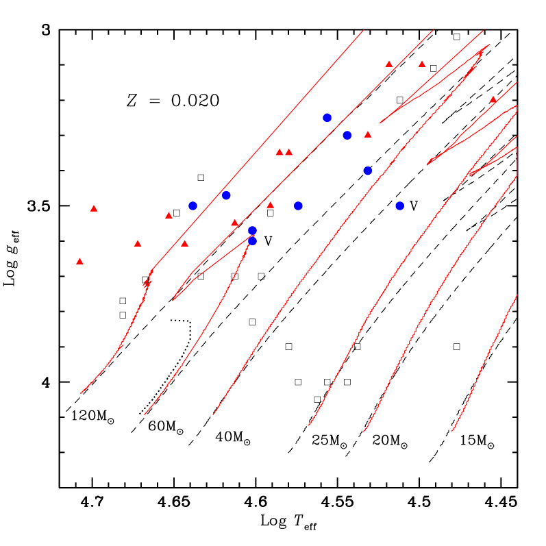
Figure 16: Evolutionary tracks in the $\log g_{\rm eff}$ versus $\log T_{\rm eff}$ plane where $g_{\rm eff}$ is the effective surface gravity. The dashed and continuous lines are for the non–rotating and rotating ($v_{\rm ini}$ = 300 km s^-1) models respectively. The dotted track corresponds to the fast rotating 60 M_⊙ plotted on Fig. 15. Only the beginning of the evolution is shown. The positions of the stars observed by Herrero et al. (He92 (1992), He99 (1999), He20 (2000)) are indicated with the same symbols as in Fig. 15.

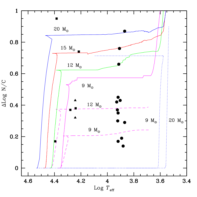
Figure 17: Evolution as a function of log $T_{\rm eff}$ of $\Delta\log{\rm N\over\rm C}=\log({\rm N/C})-\log({\rm N/C})_{i}$, where N and C are the surface abundances (in number) of nitrogen and carbon respectively, the index $i$ indicates initial values. The continuous tracks correspond to rotating stellar models with $v_{\rm ini}$ = 300 km s^-1. The dashed and dotted lines are respectively for initial $v_{\rm ini}$ = 200 and 0 km s^-1. Only parts of the tracks with $v_{\rm ini}$ = 200 km s^-1 are shown. The initial masses are indicated. The solid squares and triangles correspond to observed blue supergiants by Gies and Lambert (gi92 (1992)) and Lennon (le94 (1994)) as reported by Venn (1995b ). The solid circles show the positions of galactic A–type supergiants observed by Venn (1995a , b).

7.2 Comparisons with the surface abundances of supergiants

Most blue supergiants present surface enrichments. For instance, Walborn (wa76 (1976), wa88 (1988)) showed that ordinary OB supergiants have He– and N– enrichments as a result of CNO processing. Only the small group of peculiar OBC–stars has the normal cosmic abundance ratios (cf. also Howarth and Prinja ho89 (1989); Herrero et al. He92 (1992); Gies and Lambert gi92 (1992); Lennon le94 (1994)). A possibility to explain the He– and N–enrichments in supergiants would be that blue supergiants are on a blue loop after a first red supergiant stage where dredge–up has occurred producing the observed surface enrichments. However as we shall see below, this does not appear as the good explanantion at least for some of the observed enrichments.

Fig. 17 illustrates the changes of the nitrogen to carbon ratios N/C from the ZAMS to the red supergiant stage for stars in the mass range from 9 to 20 M_⊙. The N/C ratio appears as the most sensitive observable parameter. For non–rotating stars, the surface enrichment in nitrogen only occurs when the star reaches the red supergiant phase; there, CNO elements are dredged–up by deep convection. The behaviour is the same as for the He–enrichments discussed above. For rotating stars, N–excesses already occur during the MS phase and they are larger for higher rotation and initial stellar masses. At the end of the MS phase of the 12 M_⊙ model, the N/C ratio is enhanced by factors 2.4 and 4.3 for $v_{\rm ini}$ = 200 and 300 km s^-1 respectively. These factors are increased up to 4 and 7.1 for the 20 M_⊙ models with the same $v_{\rm ini}$.

On Fig. 17 we plot also some observations of supergiants performed by Gies and Lambert (gi92 (1992)), Lennon (le94 (1994)) and Venn (1995a b). The plotted values are $\Delta\log{\rm N/C}=[{\rm N/C}]_{*}-[{\rm N/C}]_{B}$, where the abundance ratios in number are measured at the surface of the star ($*$), and at the surface of main sequence B–stars ($B$) supposed to have retained their pristine cosmic abundances. Gies and Lambert (gi92 (1992)) provide “LTE” and “NLTE” N/C ratios. We plot here the smaller “LTE” ratios since, for the stars in common with the Lennon sample, they are similar to Lennon’s results (see the discussion in Venn 1995b ). From the positions of the observed stars in the $\log g_{\rm eff}$ versus $\log T_{\rm eff}$ diagram, one obtains that the range of initial masses for the A–type supergiants shown on Fig. 17 are between 5 and 20 M_⊙.

From Fig. 17, one notes first that at the $T_{\rm eff}$ of the observed supergiants, non–rotating stellar models predict no enrichment at all unless there is a blue loop. However it is not likely that all the observed points are at the tip of a blue loop. Indeed some of the stars have initial masses above 15 M_⊙ and, at solar metallicity, current grids of models (Arnett ar91 (1991); Schaller et al. sch92 (1992); Alongi et al. al93 (1993); Brocato and Castellani br93 (1993)) only predict blue loops for masses equal or lower than 15 M_⊙. Moreover many of the observed stars have N/C ratios too low to result from a first dredge–up episode (see for instance the position of the blue loop of the non–rotating 9 M_⊙ model in Fig. 17). Therefore Venn (1995b ) suggested that at least those stars presenting the lowest N/C ratios are on their way from the MS to the red giant branch and have undergone some mixing in the early stage of their evolution. If such stars are not at all accounted for by standard evolutionary tracks, rotating models can naturally reproduce their observed surface abundances as can be seen on Fig.17.

Moreover as already noted above, theory predicts larger excesses for higher masses, a result in agreement with the suggestion of Takeda and Takeda–Hidai (ta95 (1995)) recently confirmed by McErlean et al. (mc99 (1999)).

8 Conclusion

Mass loss by stellar winds and rotational mixing in the stellar interior are certainly the two hydrodynamical phenomena which most deeply affect the evolution of massive stars. Far from being a small refinement in the physics of stellar interior, rotation appears as an essential ingredient of future grids of stellar models. In particular among the important points wich are not discussed here but which will be studied in more details in forthcoming papers are the effects of rotation on the population of red and blue supergiants at various metallicities, on the evolutionary scenarios leading to the formation of Wolf–Rayet stars (Maeder 1987; Fliegner and Langer 1995; Meynet 2000b) and on the stellar yields (Heger et al. 2000). These questions are important for a better understanding of starbursts regions and of the chemical evolution of galaxies.

References

- (1) Alongi M., Bertelli G., Bressan A., Chiosi C., Fagotto F., 1993, A&AS 97, 851
- (2) Arnett D., 1991, ApJ 383, 295
- (3) Barrado y Navascués D., Stauffer J.R., Patten B.M., 1999, ApJ 522, L53
- (4) Bernasconi P., Maeder A., 1996, A&A 307, 829
- (5) Bertelli G., Bressan A., Chiosi C., 1985, A&A 150, 33
- (6) Brocato E., Castellani V., 1993, ApJ 410, 99
- (7) Canuto V.M., 1998, ApJ 508, 767
- (8) Canuto V.M., 2000, ApJ 534, L113
- (9) Chaboyer B., Demarque P., Pinsonneault M.H., 1995a, ApJ 441, 865
- (10) Chaboyer B., Demarque P., Pinsonneault M.H., 1995b, ApJ 441, 876
- (11) Chaboyer B., Zahn J.P., 1992, A&A 253, 173
- (12) Chin C.W., Stothers R.B., 1990, ApJS 73, 821
- (13) Collins G.W., Sonneborn G.H., 1977, ApJS 34, 41
- (14) de Jager C., Nieuwenhuijzen H., van der Hucht K.A., 1988, A&AS 72, 259
- (15) Denissenkov P.A., Ivanova N.S., Weiss A., 1999, A&A 341, 181
- (16) Endal A.S., Sofia S., 1976, ApJ 210, 184
- (17) Endal A.S., Sofia, S., 1978, ApJ 220, 279
- (18) Fliegner J., Langer N., 1995. Models of rotating Wolf–Rayet stars. In: van der Hucht K.A., Williams P.M. (eds.) IAU Symp. 163, Wolf–Rayet Stars: Binaries, Colliding Winds, Evolution, Kluwer, p. 326
- (19) Friend D.B., Abbott D.C., 1986, A&A 311, 701
- (20) Fukuda I. 1982, PASP 92, 271
- (21) Gies D.R., Lambert D.L., 1992, ApJ 387, 673
- (22) Glatzel W., 1998, A&A 324, 210
- (23) Heger A., Langer N., 1998, A&A 324, 210
- (24) Heger A., Langer N., Woosley S.E., 2000, ApJ 528, 368
- (25) Herrero A., Corral L.J., Villamariz M.R., Martin E.L., 1999, A&A 348, 542
- (26) Herrero A., Kudritzki R.P., Vilchez J.M., Kunze D., Butler K., Haser S., 1992, A&A 261, 209
- (27) Herrero A., Puls J., Villamariz M.R., 2000, A&A 354, 193
- (28) Howarth I.D., Prinja R.K., 1989, ApJS 69, 527
- (29) Howarth I.D., Siebert K.W., Hussain G.A.J., Prinja R.K., 1997, MNRAS 284, 265
- (30) Kippenhahn R., 1977, A&A 58, 267
- (31) Kippenhahn R., Thomas H.C., 1970, A Simple Method for the Solution of the Stellar Structure Equations Including Rotation and Tidal Forces. In: Slettebak A. (ed.) Proc. IAU Coll. 4, Stellar Rotation. Gordon and Breach Science Publishers, p. 20
- (32) Kippenhahn R., Weigert A., 1990, Stellar Structure and Evolution, Springer Verlag, Berlin
- (33) Lamers H., Cassinelli J. P., 1996, Mass Loss from Stars. In: Leitherer C., Fritze-von-Alvensleben U., Huchra J. (eds.) From Stars to Galaxies: The Impact of Stellar Physics on Galaxy Evolution. ASP Conf. Series 98, p. 162
- (34) Lamers H.J.G.L.M., Leitherer C., 1993, ApJ 412, 471
- (35) Langer N., 1989, A&A 220, 135
- (36) Langer N., 1992, A&A 265, L17
- (37) Langer N., 1997, The Eddington Limit in Rotating Massive Stars. In: Nota A., Lamers H. (eds.) Luminous Blue Variables: Massive Stars in Transition. ASP Conf. Series 120, p. 83
- (38) Langer N., 1998, A&A 329, 551
- (39) Langer N., Fricke K.J., Sugimoto D., 1983, A&A 126, 207
- (40) Langer N., Maeder A., 1995, A&A 295, 685
- (41) Lanz T., de Koter A., Hubeny I., Heap S.R., 1996, ApJ 465, 359
- (42) Lauterborn D., Refsdal S., Weigert A., 1971, A&A 10, 97
- (43) Lennon D.J., 1994, Space Sci. Rev. 66, 127
- (44) Lyubimkov, L.S., 1996, Astroph. Sp. Sci. 243, 329
- (45) Maeder A., 1971, A&A 10, 354
- (46) Maeder A., 1981, A&A 102, 401
- (47) Maeder A., 1987, A&A 178, 159
- (48) Maeder A., 1995a, Population I Stellar Structure and Evolution: facing the lingering difficulties to make a step forward. In: Stobie R.S., Whitelock P.A. (eds) Astrophysical applications of stellar pulsation. ASP Conf. Series 83, p. 1
- (49) Maeder A., 1995b, A&A 299, 84
- (50) Maeder A., 1997, A&A 321, 134 (Paper II)
- (51) Maeder A., 1998, The Physics of Rotational Mixing in Massive Stars. In: Howarth I. (ed.) Boulder-Munich II: Properties of Hot, Luminous Stars. ASP Conf. Ser. 131, p. 85
- (52) Maeder A., 1999, A&A 347, 185 (Paper IV)
- (53) Maeder A., Meynet G., 1989, A&A 210, 155
- (54) Maeder A., Meynet G., 1996, A&A 313, 140
- (55) Maeder A., Meynet G., 2000a, A&A, in press (Paper VI)
- (56) Maeder A., Meynet G., 2000b, ARAA 38, in press
- (57) Maeder A., Peytremann E., 1970, A&A 7, 120
- (58) Maeder A., Zahn J.P., 1998, A&A 334, 1000 (Paper III)
- (59) Maeder A., Grebel E., Mermilliod J.C., 1999, A&A 346, 459
- (60) Martin E.L., Basri G., Gallegos J.E., Rebolo R., Zapatero-Osorio M.R., Bejar V.J.S., 1998, ApJ 499, L61
- (61) Mathys G., 1999, Direct Observational Evidence for Magnetic Fields in Hot Stars. In: Wolf B., Stahl O., Fullerton A.W. (eds.) Proc. IAU Coll. 169, Variable and Non-spherical Stellar Winds in Luminous Hot Stars, Springer, Berlin, p. 95
- (62) McErlean N.D., Lennon D.J., Dufton P.L., 1998, A&A 329, 613
- (63) McErlean N.D., Lennon D.J., Dufton P.L., 1999, A&A 349, 553
- (64) Mestel L., 1965, In Stellar Structure, Eds. LH Aller & DB McLaughlin, Univ. Chicago Press, p. 465
- (65) Meynet G., 1998, Massive-Star Models With Rotation: New Numerical Results. In: Howarth I. (ed.) Boulder-Munich II: Properties of Hot, Luminous Stars. ASP Conf. Ser. 131, p. 96
- (66) Meynet G., 1999, Rotation and Wolf–Rayet Star Formation. In: Wolf B., Stahl O., Fullerton A.W. (eds.) Proc. IAU Coll. 169, Variable and Non-spherical Stellar Winds in Luminous Hot Stars, Springer, Berlin, p. 377
- (67) Meynet G., 2000a, Massive star evolution with rotation: effects on surface abundances. In: Pallavicini R., Micela G., Sciortino (eds.) Stellar Clusters and Associations. ASP Conf. Ser. 198, p. 3
- (68) Meynet G., 2000b, Evolution of rotating massive stars into the Wolf–Rayet phase at solar metallicity. In: Lançon A. (ed.) Massive Stellar Clusters. ASP Conf. Ser., in press
- (69) Meynet G., Maeder A., 1997, A&A 321, 465 (Paper I)
- (70) Meynet G., Maeder A., Schaller G., Schaerer D., Charbonnel C., 1994, A&AS 103, 97
- (71) Nieuwenhuijzen H., de Jager C., 1988, A&A 203, 355
- (72) Nugis T., Crowther P.A., Willis A.J., 1998, A&A 333, 956
- (73) Penny L.R., 1996, ApJ 463, 737
- (74) Penny L.R., Gies D.R., Bagnuolo W.G., 1999, Discrepancies between observational and theoretical parameters of three O-type binaries. In: van der Hucht K.A., Koenigsberger G., Eenens P.R.J. (eds.) IAU Symp. 193, Wolf–Rayet Phenomena in Massive Stars and Starburst Galaxies. ASP Conf. Ser., p. 86
- (75) Pinsonneault M.H., Kawaler S.D., Sofia S., Demarque P., 1989, ApJ 338, 424
- (76) Sackmann I.J., Anand S.P.S., 1970, ApJ 162, 105
- (77) Schaller G., Schaerer D., Meynet G., Maeder A., 1992, A&AS 96, 269
- (78) Schmutz W., 1997, A&A 321, 268
- (79) Schwarzschild M., 1958, Structure and evolution of the stars, Princeton University Press, Princeton, pp. 183
- (80) Slettebak A., 1970, Stellar rotation. In: Slettebak A. (ed.) Proc. IAU Coll. 4, Stellar rotation. Reidel, Dordrecht, P. 3
- (81) Smith K.C., Howarth I.D., 1998, MNRAS 299, 1146
- (82) Stothers R.B., Chin C.W., 1979, ApJ 233, 267
- (83) Takeda Y., Takada–Hidai M., 1995, PASJ 47, 169
- (84) Talon S., Zahn J.P., 1997, A&A 317, 749
- (85) Talon S., Zahn J.P., Maeder A., Meynet G., 1997, A&A, 322, 209
- (86) Tassoul J.L., 1990, The Effects of Rotation on Stellar Structure and Evolution. In: Willson L.A., Stalio R. (eds.) Angular Momentum and Mass Loss for Hot Stars. Kluwer Acad. Publ., p. 7
- (87) Urpin V.A., Shalybkov D.A., Spruit H.C., 1996, A&A 306, 455
- (88) Vardya M.S., 1985, ApJ 299, 255
- (89) Vauclair S., 1999, A&A 351, 973
- (90) Venn K.A., 1995a, ApJ 449, 839
- (91) Venn K.A., 1995b, ApJS 99, 659
- (92) Venn K.A., McCarthy J.H., Lennon D.J., Kudritzki R.P., 1998, A-Supergiant Abundances in Local-Group Galaxies. In: Howarth I. (ed.) Boulder-Munich II: Properties of Hot, Luminous Stars. ASP Conf. Ser. 131, p. 177
- (93) Venn K.A., 1999, ApJ 518, 405
- (94) Villamariz M.R., Herrero A., 1999, The effect of micro–turbulence in O–type star analyses. In: van der Hucht K.A., Koenigsberger G., Eenens P.R.J. (eds.) IAU Symp. 193, Wolf–Rayet Phenomena in Massive Stars and Starburst Galaxies. ASP Conf. Ser., p. 265
- (95) von Zeipel H., 1924, MNRAS 84, 665
- (96) Walborn N.R., 1976, ApJ 205, 419
- (97) Walborn N.R., 1988, Evolutionary Helium and CNO Anomalies in the Atmospheres and Winds of Massive Hot Stars. In: Nomoto K. (eds.) Proc. IAU Coll. 108, Atmospheric Diagnostics of Stellar Evolution. Chemical Peculiarity, Mass Loss, and Explosion. Springer-Verlag, Berlin, p. 70
- (98) Zahn J.P., 1974, Rotational instabilities and stellar evolution. In: Ledoux P. (ed.) Proc. IAU Symp. 59, Stellar instability and evolution. Reidel, Dordrecht, p. 185
- (99) Zahn J.P., 1992, A&A 265, 115