X-ray colour maps of the cores of galaxy clusters

Abstract

We present an analysis of X-ray colour maps of the cores of clusters of galaxies, formed from the ratios of counts in different X-ray bands. Our technique groups pixels lying between contours in an adaptively-smoothed image of a cluster. We select the contour levels to minimize the uncertainties in the colour ratios, whilst preserving the structure of the object. We extend the work of Allen & Fabian (1997) by investigating the spatial distributions of cooling gas and absorbing material in cluster cores. Their sample is almost doubled: we analyse archive ROSAT PSPC data for 33 clusters from the sample of the 55 brightest X-ray clusters in the sky. Many of our clusters contain strong cooling flows. We present colour maps of a sample of the clusters, in addition to adaptively-smoothed images in different bands. Most of the cooling flow clusters display little substructure, unlike several of the non-cooling-flow clusters.

We fitted an isothermal plasma model with galactic absorption and constant metallicity to the mid-over-high energy colours in our clusters. Those clusters with known strong cooling flows have inner contours which fit a significantly lower temperature than the outer contours. Clusters in the sample without strong cooling flows show no significant temperature variation. The inclusion of a metallicity gradient alone was not sufficient to explain the observations. A cooling flow component plus a constant temperature phase did account for the colour profiles in clusters with known strong cooling flow components. We also had to increase the levels of absorbing material to fit the low-over-high colours at the cluster centres. Our results provide more evidence that cooling flows accumulate absorbing material. No evidence for increased absorption was found for the non-cooling-flow clusters.

1 Introduction

Clusters of galaxies are among the largest dynamical objects in the universe. They contain large quantities of virilised gas (the intracluster medium, or ICM) at temperatures of the order of $10^{7}$–$10^{8}$ K, heated by their initial gravitational collapse. Due to this gas they are powerful emitters of X-rays from bremsstrahlung and line emission. The gas masses of rich clusters exceed $10^{14}\>M_{\odot}$, and they can emit over $10^{45}\textrm{ erg s}^{-1}$ in X-rays.

The radiative cooling time, $t_{\mathrm{cool}}$, is shortest in the densest regions, at the centre of a cluster, and is often found to be less than the plausible age of the cluster, i.e. the time since its last major interaction, which is a significant fraction of the Hubble time. As the gas cools, its temperature decreases, but its density must rise to maintain hydrostatic equilibrium. This is achieved by the gas above flowing in. This is known as a cooling flow (See Fabian 1994 for a review).

Observations have shown that cooling flows are inhomogeneous. The mass drops out of the flow into a form which does not emit X-rays. The exact destination and final form of this gas has not been determined, but magnetic fields are probably important in determining, and constraining, the structure of cooled gas.

The rate of the mass of gas cooling out at a certain radius is known as the mass deposition rate, $\dot{M}(r)$. This value can total from 10–1000 $M_{\odot}\textrm{ yr}^{-1}$. The mass deposition rate can be estimated by assuming that all the luminosity within the cooling radius, where the cooling time is less than the age of the cluster, is due to the cooling gas radiation, plus the $P\mathrm{d}V$ work done on the gas as it enters that radius. The relationship between the mass deposition rate and radius is found to be roughly linear, as the surface brightness profiles are not as centrally peaked as would be expected for a homogeneous cooling flow.

Allen & Fabian (1997) undertook a study of the spatial distributions of cooling gas and intrinsic X-ray absorbing material in a sample of nearby clusters, using X-ray colour profiles, formed from the ratio of flux in selected bands, using data from the ROSAT Position Sensitive Proportional Counter (PSPC). They found that the profiles indicated that there were significant central concentrations of cooling gas in their cooling flow clusters, becoming approximately isothermal at larger radii. Their profiles also showed large levels of X-ray absorption in the cluster cores, increasing with decreasing radius.

The bands they examined are listed in Table 1, which they combined to form two X-ray colour ratios, $B/D$ and $C/D$. To analyse the observations, they calculated theoretical curves for the colours as functions of temperature and metallicity, with a uniform screen to model the absorbing column density. They modelled both colours with isothermal and cooling gas models. In Section 4 we reevaluate these functions using more recent plasma models.

To demonstrate the presence of distributed cooling gas in the central regions of cooling flow clusters, they used the $C/D$ profile, and the $B/D$ ratio to demonstrate the presence of intrinsic X-ray absorbing gas. They found the absorbing material only partially covers the X-ray emitting region.

Table 1: Definition of the energy bands (Allen & Fabian 1997)

Band	Energy range (keV)
$A_{1}$	0.10–0.20
$A_{2}$	0.20–0.40
$B$	0.41–0.79
$C$	0.80–1.39
$D$	1.40–2.00
$F$	0.41–2.00

In this paper, we extend the analysis of Allen & Fabian (1997). Instead of making a simple radial profile of each cluster, we have developed a technique to take account of the two-dimensional structure of the image. Simple binning works in areas of high flux, where the errors created in forming ratios of counts are small. In low flux regions, the number of pixels required to bin destroys most of the spatial information in the image. Our method attempts to make statistically useful X-ray colours, whilst preserving spatial resolution.

2 Observations and colour map analysis

We analysed archival ROSAT PSPC data for a sample of 33 clusters. The clusters we examined are shown in Table 2. The sample was mainly chosen to include known strong cooling flow clusters (from Peres et al. 1998), with a few non-cooling-flow clusters for comparison.

We used the bands of Allen & Fabian (1997) in our analysis. These bands are optimised for the study of cooling gas. This precluded the use of the extended object analysis package of Snowden & Kuntz (1998), although we made use of some modified versions of a few of their routines.

The full analysis procedure for each cluster is as follows.

1. We removed time periods from the observation where the Master Veto count rate averaged over $\sim 30$ s was greater than 220 counts $\mathrm{s}^{-1}$ (Snowden et al. 1994).

2. A modified version of Snowden’s cast_data routine was used to create $512\times 512$ pixel images of the cluster, at a pixel size of approximately $15\times 15\textrm{ arcsec}^{2}$. We created images of the cluster in the $B$, $C$ and $D$ bands from Table 1.

3. We corrected the $B$, $C$ and $D$ band images for background counts (Section 2.2).

4. An adaptively-smoothed image (Section 2.1) was made of the central region of the cluster, in the high energy $D$ band. We created an image of size $64\times 64$, or occasionally $128\times 128$ pixels, depending on the extent of the cluster.

5. We created linear contours in the adaptively-smoothed image, by simply taking the difference between the maximum and minimum count rates, and dividing by the number of contours.

6. The counts for those pixels between each two neighbouring contours was added, in each of the background corrected $B$, $C$ and $D$ images.

7. We used the count totals to generate average $B/D$ and $C/D$ colours for each contour. The error on each result is:

   $$\left(\frac{\sigma_{r}}{r}\right)^{2} = \frac{\sum_{\mathrm{pixels}}\left(N_{i}^{X}+C_{i}^{X}\right)}{\left[\sum_{\mathrm{pixels}}\left(N_{i}^{X}-C_{i}^{X}\right)\right]^{2}}+$$ (1)

   $$\frac{\sum_{\mathrm{pixels}}\left(N_{i}^{Y}+C_{i}^{Y}\right)}{\left[\sum_{\mathrm{pixels}}\left(N_{i}^{Y}-C_{i}^{Y}\right)\right]^{2}},$$

   where $r$ is the $X/Y$ average ratio, and $\sigma_{r}$ is the error on the ratio. $N_{i}^{X}$ is the uncorrected number of photons in pixel $i$ in band $X$, and $C_{i}^{X}$ is the background correction for pixel $i$ in band $X$. This expression does not take account of systematic background uncertainties. We ignored pixels that were suspected to contain point sources (Section 2.2) outside the core.

8. A Monte Carlo procedure was used to change the contour levels in the adaptively-smoothed image to minimize the total error squared in the contours for both colours, or the value

   $$x=\sum_{\mathrm{contours}}\left\{\left[\sigma_{(B/D)_{i}}\right]^{2}+\left[\sigma_{(C/D)_{i}}\right]^{2}\right\}.$$ (2)

   The result of moving the contour levels to minimize $x$ creates contour levels which contain similar numbers of counts and signal to noise ratios. The procedure produces colour ratios with roughly equal fractional uncertainties for each contour.

We used six contours to process the cluster images. This was a good compromise between showing detail and keeping statistical errors low. The results were stable to small changes in the number of contours.

2.1 Adaptive smoothing

Adaptive smoothing is a technique to smooth an image and retain significant small-scale structure (Ebeling, White & Rangarajan 2000). Smoothing is required because it is often the case, especially in X-ray data, that there are few photons per pixel. However, convolving an image with a Gaussian kernel leads to broadening of features and loss of small-scale structure. An algorithm is required which retains information on all scales.

An adaptive kernel smoothing (AKS) algorithm applies a kernel with a varying size to an image. A part of the image with few counts is smoothed with a large kernel, whilst a part with many counts is smoothed with a small kernel. The algorithm decides what is the ‘natural’ smoothing scale for a part of an image. AKS algorithms differ on how they choose an appropriate kernel size. We used the asmooth algorithm of Ebeling, White & Rangarajan (2000) to adaptively smooth our cluster images. asmooth is unusual in that it uses the local signal-to-noise ratio to adjust the size of the kernel. The minimum signal-to-noise ratio of the part of the image smoothed by the kernel is a parameter to the algorithm. A level of 6-$\sigma$ seemed to produce the best results; it appeared not to generate false detail from spurious pixels. We used a Gaussian rather than top-hat adaptive kernel.

Other methods for revealing structure in data include wavelet analysis (Starck & Pierre 1998). Different methods have other advantages, but the asmooth algorithm is particularly simple and quick to perform.

2.2 Background removal

The raw data contains counts not from the observed source. These background counts, sources of which are listed below, must be removed.

1. The X-ray background, which comes through the aperture of the telescope, and is observed with the same vignetting response of the telescope as the object. This includes solar and extragalactic background emission.

2. The particle background (Plucinsky et al. 1993) is diffuse and is caused by high energy cosmic rays. The flux of the particle background is approximately constant across the detector.

These components vary in strength with X-ray energy, so they must be removed to make X-ray colours.

To estimate the background we took the average count from the 30–35 arcmin region, beyond the ‘ribs’ in the field of the PSPC. From this count we subtracted an estimate of the particle background from Plucinsky et al. (1993), of $4\times 10^{-6}$ counts $\textrm{pixel}^{-1}$ $\textrm{s}^{-1}$ $\textrm{arcmin}^{-2}$ $\textrm{keV}^{-1}$. We corrected the result for vignetting. The corrected count and the particle background was removed from all pixels.

Accounting for the total background reduces the scatter of the observed data points. It also hardens the emission from the outermost parts of clusters which emit few photons.

Three clusters, A2142, A1795 and A2029, contained obvious point sources in their fields outside the cluster core. We removed the point sources using a mask which excluded the affected region around them. Those pixels inside the mask were not included in the sum of counts inside a contour.

Table 2: The sample of clusters examined. $z$ is the redshift taken from the NASA/IPAC Extragalactic Database (NED), and the values of $\dot{M}$, the mass deposition rate, are PSPC observation derived values taken from Peres et al. (1998), as are the central cooling time values, $t_{\mathrm{cool}}$. The sequence identification and exposure time give PSPC observation details. $S(B/D)$ and $S(C/D)$ are the significance of a colour gradient, larger values imply a larger colour gradient (Section 3). The clusters are listed in cooling flow flux order, $\dot{M}/z^{2}$.

Cluster	Sequence ID	Exposure/s	$z$	$\dot{M}/(M_{\odot}\>\mathrm{yr}^{-1})$	$t_{\mathrm{cool}}/\textrm{Gyr}$	$S(B/D)$	$S(C/D)$
Virgo	rp800187n00	10536	0.0037	$39^{+2}_{-9}$	$0.2^{+0.0}_{-0.0}$	4.9	21
Perseus	rp800186n00	4711	0.0183	$556^{+33}_{-24}$	$0.9^{+0.0}_{-0.0}$	5.9	8.4
2A 0335+096	rp800083n00	10220	0.0349	$325^{+32}_{-43}$	$0.9^{+0.0}_{-0.0}$	2.6	7.1
Centaurus	rp800192n00	7793	0.0109	$30^{+10}_{-5}$	$0.8^{+0.0}_{-0.0}$	1.9	14
A2199	rp800644n00	40999	0.030	$154^{+18}_{-8}$	$1.9^{+0.0}_{-0.1}$	7.8	10
Ophiuchus	rp800279n00	3932	0.028	$127^{+48}_{-94}$	$3.0^{+0.4}_{-0.3}$	-1.2	0.3
Klemola 44	rp800354n00	3353	0.0283	$87^{+25}_{-19}$	$2.3^{+0.6}_{-0.2}$	-1.6	0.1
A2052	rp800275n00	6211	0.0348	$125^{+26}_{-6}$	$2.5^{+0.1}_{-0.1}$	2.1	4.6
A262	rp800254n00	8686	0.0164	$27^{+4}_{-3}$	$1.5^{+0.1}_{-0.1}$	2.2	5.1
PKS 0745-191	rp800623n00	10473	0.1028	$1038^{+116}_{-68}$	$2.2^{+0.1}_{-0.1}$	2.6	2.7
A1060	rp800200n00	15764	0.0124	$15^{+5}_{-7}$	$4.7^{+0.4}_{-0.3}$	0.3	0.1
A1795	rp800105n00	36273	0.0627	$381^{+41}_{-23}$	$1.9^{+0.1}_{-0.1}$	4.6	5.9
Hydra-A	rp800318n00	18398	0.0522	$264^{+81}_{-60}$	$2.0^{+0.0}_{-0.0}$	3.8	5.5
A2029	rp800249n00	12542	0.0767	$556^{+44}_{-73}$	$2.9^{+0.1}_{-0.1}$	4.4	5.2
A496	rp800024n00	8857	0.033	$95^{+13}_{-12}$	$1.8^{+0.1}_{-0.1}$	1.4	3.8
MKW3	rp800128n00	9984	0.0449	$175^{+14}_{-46}$	$3.0^{+0.1}_{-0.1}$	-0.1	0.8
A478	rp800193n00	21969	0.0882	$616^{+63}_{-76}$	$2.8^{+0.1}_{-0.1}$	-0.8	2.1
A85	rp800250n00	10238	0.0521	$198^{+53}_{-52}$	$2.4^{+0.1}_{-0.1}$	1.5	2.9
A3112	rp800302n00	7598	0.0746	$376^{+80}_{-61}$	$1.9^{+0.1}_{-0.1}$	1.4	3.6
Cygnus-A	rp800622n00	9442	0.057	$244^{+26}_{-22}$	$2.6^{+0.1}_{-0.1}$	0.6	1.6
AWM7	rp800168n00	13088	0.0172	$41^{+6}_{-6}$	$1.9^{+0.2}_{-0.2}$	-0.4	2.2
A4059	rp800175n00	5439	0.0478	$130^{+27}_{-21}$	$3.4^{+0.6}_{-0.4}$	0.9	1.9
A3571	rp800287n00	6062	0.0391	$72^{+56}_{-31}$	$5.8^{+0.9}_{-1.0}$	6.7	3.4
A2597	rp800112n00	7163	0.0824	$271^{+41}_{-41}$	$2.3^{+0.1}_{-0.1}$	-0.3	1.4
A644	rp800379n00	10246	0.0704	$189^{+106}_{-35}$	$6.8^{+0.4}_{-0.4}$	2.8	1.4
A2204	rp800281n00	5357	0.1523	$852^{+127}_{-82}$	$3.1^{+0.1}_{-0.1}$	2.8	3.4
A2142	rp150084n00	7734	0.0899	$350^{+66}_{-133}$	$5.2^{+0.4}_{-0.3}$	1.0	1.0
A3558	rp800076n00	29490	0.0478	$40^{+39}_{-10}$	$10.2^{+0.3}_{-0.2}$	-0.2	1.2
A401	rp800235n00	7457	0.0743	$42^{+82}_{-42}$	$10.6^{+4.0}_{-1.8}$	-0.6	-1.3
Coma	rp800005n00	21140	0.0232	$0^{+1}_{-0}$	$17.7^{+6.7}_{-4.1}$	1.7	0.9
A754	rp800550n00	8156	0.0542	$0^{+29}_{-0}$	$15.0^{+3.1}_{-2.2}$	1.6	2.5
A2256	rp800162a01	4747	0.0581	$0^{+14}_{-0}$	$15.0^{+4.0}_{-3.6}$	0.2	0.9
A119	rp800251n00	15197	0.044	$0^{+2}_{-0}$	$19.2^{+12.2}_{-8.6}$	-0.9	-1.8

Table 3: Mean distance of the pixels in each contour from the cluster centre. Distances are measured in pixels (15 arcsec). The contours are numbered from 1 (inner) to 6 (outer). Clusters marked with an asterix (*) were examined using a $128\times 128$ pixel adaptively smoothed image, rather than a $64\times 64$ image.

Cluster	1	2	3	4	5	6
2A 0335+096	2.1	3.8	5.9	8.7	13.8	28.7
A1060*	6.9	13.2	19.2	26.5	37.0	60.7
A119*	7.5	14.6	20.8	27.5	37.0	60.4
A1795	2.6	4.2	6.6	9.6	14.7	28.9
A2029	2.7	4.3	6.4	9.5	13.7	28.5
A2052	3.0	5.0	7.9	10.5	14.9	28.9
A2142	3.1	5.2	8.3	12.2	18.3	29.5
A2199	3.6	7.0	10.5	14.4	20.3	31.1
A2204	2.8	2.9	3.6	5.5	8.0	26.9
A2256*	7.4	11.9	16.7	20.8	25.6	56.1
A2597	2.4	2.9	3.7	5.3	8.1	27.0
A262*	6.3	11.8	18.1	24.8	33.4	59.1
A3112	3.3	3.7	5.2	8.0	13.1	28.5
A3558*	7.1	12.5	17.0	21.0	27.6	56.8
A3571*	5.5	10.2	14.4	21.7	32.1	58.0
A401	3.0	6.4	9.7	12.8	16.9	29.6
A4059	3.3	5.7	8.5	11.5	17.5	30.3
A478	2.4	3.6	5.1	7.6	11.2	27.8
A496	2.8	5.7	9.4	13.9	20.1	31.0
A644	3.8	6.1	8.7	11.8	16.4	29.0
A754*	12.0	25.7	27.7	30.7	36.6	57.2
A85	2.9	5.9	10.0	14.0	19.5	30.8
AWM7*	7.9	14.4	21.1	27.7	36.5	60.0
Centaurus*	5.7	12.3	18.5	27.2	39.2	60.9
Coma*	14.0	22.5	29.4	36.7	46.6	63.0
Cygnus A	4.6	5.3	6.2	8.8	16.5	29.5
Hydra A	2.6	3.8	6.7	9.6	13.4	28.4
KLEM44	4.3	6.0	8.9	12.4	17.8	29.8
MKW3	2.4	4.7	7.0	9.2	12.9	28.2
Ophiuchus	7.3	12.2	15.2	19.1	24.4	31.3
Perseus*	4.2	8.4	13.5	22.2	34.8	59.3
PKS 0745-191	2.4	3.1	4.0	6.2	9.6	27.3
Virgo*	7.4	14.2	21.7	30.2	41.1	62.2

3 Results

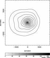
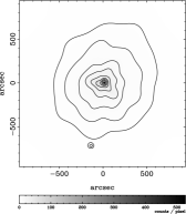
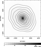
We created adaptively-smoothed images of the sample of clusters in the $B$, $C$ and $D$ bands, using an asmooth minimum significance of 6-$\sigma$. Fig. 1, 2 and 3 show the images for the Perseus, Virgo and A2199 clusters, respectively. ROSAT HRI images of the centres of the Perseus cluster, NGC 1275, and the Virgo cluster, M87, have been examined by Böhringer et al. (1993, 1995), respectively. They found the thermal plasma was displaced by the radio lobes of NGC 1275 at the centre of the Perseus cluster.

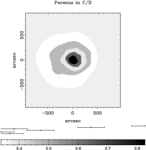
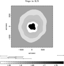
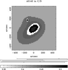
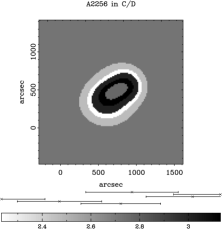
Fig. 4 and 5 are colour contour maps of the Perseus and Virgo clusters. The maps show the average X-ray colours between each of six contours. The scale below each map shows the value and statistical uncertainty of the colour of each contour. The extreme error bars on the softest and hardest points are not shown on the scales. Note that darker shades in these plots indicate softer emission. Table 3 shows the mean physical distance from the cluster centre of each contour in each cluster in pixels. It also identifies which clusters were examined using a $64\times 64$ pixel image or a $128\times 128$ image.

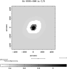
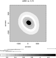
Fig. 6 shows a sample of six colour contour maps. Four of the clusters are non-cooling-flow clusters, showing interesting features. Two are cooling flow clusters, which make up most of our sample, and they reveal little substructure. The point source in A2142 is shown, but is not included in the contour statistics.

Fig. 7 and 8 show the average $B/D$ and $C/D$ colours for the contours of each of the sample of clusters. The clusters are listed in decreasing cooling flow flux order ($\dot{M}/z^{2}$, where $\dot{M}$ is the mass deposition rate, and $z$ is the redshift of the cluster) using the PSPC $\dot{M}$ values obtained by Peres et al. (1998). However, some of the clusters have highly uncertain mass deposition rates, so the ordering is not definite.

Table 2 shows a significance measure of the change in colour from the outside to the inner region for each cluster. For a cluster with contours of colour $X_{i}$, it is calculated using

$$S(X)=\frac{1}{\sqrt{3/2}\>\sigma_{X}}\left[X_{1}-\left(X_{5}+X_{6}\right)/2\right],$$ (3)

$X_{1}$ is the innermost colour value, $X_{5}$ and $X_{6}$ are the two outermost colours, $\sigma_{X}$ is the statistical uncertainty in each colour. The uncertainties are almost the same for each contour, due to our method of choosing contour levels (Section 2). $\sqrt{3/2}$ is a numerical factor to make $S(X)$ a measure of the number of 1-$\sigma$ errors. We take the mean outer two colours to decrease the chance of background contamination. The background is a large fraction of the total number of counts in the outer contour for several clusters, for example A3571, A2204, A3558 and A262.

Fig. 9 shows the variation of the significance of the $C/D$ colour, presumably due to the presence of cool gas, with the cooling flow flux, $\dot{M}/z^{2}$, for the sample of clusters. Fig. 10 shows the significance plotted against central cooling time, $t_{\mathrm{cool}}$. There is a clear anti-correlation between $t_{\mathrm{cool}}$ and the significance of a $C/D$ colour gradient. Clusters with $t_{\mathrm{cool}}\leq 2$ Gyr show colour gradients with $S(C/D)>2$. $t_{\mathrm{cool}}$ is a measure of the quality of data for a cooling flow. Cooling flow clusters with short cooling times have enough counts to make their central bins small in area.

Some of the results obtained are dependent on our choice of significance measure. If the cluster has a large soft core, as A3571, Hydra-A and A2204 seem to have in $B/D$, then using a measure based on $X_{3}+X_{4}$ instead of $X_{5}+X_{6}$ in equation (3) gives a much lower significance value. A significance based on $X_{3}+X_{4}$ would be less affected by background noise, but throws away much of the data. A more complex significance measure might be useful, but for those clusters where it might be important, noise is probably a more limiting factor.

Figure 1: Adaptively-smoothed images of the Perseus Cluster. The images are shown in bands B (left), C (middle) and D (right). The greyscale is linear and the contours are logarithmic in smoothed counts.

Figure 2: Adaptively-smoothed images of the Virgo Cluster (see Fig. 1 for a description).

Figure 3: Adaptively-smoothed images of A2199 (see Fig. 1 for a description).

Figure 4: Contour colour maps of the Perseus cluster. Areas between contours are coloured by their average X-ray colour. The points below the maps show the numerical colours, with their Poisson errors. The most central contours are the uppermost points. Darker areas indicate softer emission.

Figure 5: Contour colour maps of the Virgo cluster (see Fig. 4 for a description).

Figure 6: A selection of $C/D$ contour colour maps (see Fig. 4 for a description). The upper two clusters contain cooling flows. The others are non-cooling-flow, or low $\dot{M}$ cooling flow, clusters.

Figure 7: Variation of the ratio B/D for the sample of clusters. Each point represents the colour of a contour. The uppermost points represent the innermost contours, numbered 1.

Figure 8: Variation of the ratio C/D for the sample of clusters. Each point represents the colour of a contour. The uppermost points represent the innermost contours, numbered 1.

Figure 9: Plot of cooling flow flux, $\dot{M}/z^{2}$, against the significance measure of a colour gradient $S(C/D)$ (Section 3). The 2-$\sigma$ significance level is indicated by a dotted line.

Figure 10: Plot of the central cooling time, $t_{\mathrm{cool}}$, against the significance measure of a colour gradient $S(C/D)$ (Section 3). The 2-$\sigma$ significance level is indicated by a dotted line.

(a)		(b)
(c)		(d)

Figure 11: Theoretical predictions for the $B/D$ and $C/D$ ratios for an isothermal gas at temperatures of 1–10 keV. The lines show steps of 1 keV in temperature. The lowest temperature at the highest ratio on the $y$-axis. (a) $B/D$ and (b) $C/D$ as functions of metallicity at fixed column density ($N_{H}=10^{20}\textrm{ atom cm}^{-2}$). (c) $B/D$ and (d) $C/D$ as functions of column density at fixed metallicity ($Z=0.5Z_{\odot}$).

(a)		(b)
(c)		(d)

Figure 12: Theoretical predictions for the $B/D$ and $C/D$ ratios for an gas cooling from temperatures of 1–10 keV to 0.001 keV. The lines show steps of 1 keV in temperature. The lowest temperature at the highest ratio on the $y$-axis. (a) $B/D$ and (b) $C/D$ as functions of metallicity at fixed column density ($N_{H}=10^{20}\textrm{ atom cm}^{-2}$). (c) $B/D$ and (d) $C/D$ as functions of column density at fixed metallicity ($Z=0.5Z_{\odot}$).

(a)		(b)
(c)		(d)

Figure 13: Temperature profiles generated by fitting constant galactic obscuring column density and constant $0.3\>Z_{\odot}$ abundance to the $C/D$ colour profile. The clusters are (a) A1060 (non-cooling-flow), (b) A2199, (c) Centaurus and (d) Virgo. The errors are 1-$\sigma$, generated from the errors in $C/D$. The contours are numbered from innermost to outermost.

(a)		(b)
(c)		(d)

Figure 14: Profiles showing how the fractional cooling flow component must increase to fit the $C/D$ ratio assuming an isothermal temperature, constant galactic column density and constant $0.3\>Z_{\odot}$ abundance. The clusters are (a) A1060 (non-cooling-flow), (b) A2199, (c) Centaurus and (d) Virgo. The errors are 1-$\sigma$, generated from the errors in $C/D$. The contours are numbered from innermost to outermost.

(a)		(b)
(c)		(d)

Figure 15: Profiles showing how the intrinsic absorption must increase assuming an isothermal temperature, constant galactic column density and a constant $0.3\>Z_{\odot}$ abundance. These were calculated by assuming the cooling flow components above, and calculating the extra required column density above galactic to explain the $B/D$ ratio, assuming constant $0.3\>Z_{\odot}$ abundance. The errors are 1-$\sigma$, and were generated from the error in $B/D$, the error in the cooling flow component is ignored. The clusters are (a) A1060 (non-cooling-flow), (b) A2199, (c) Centaurus and (d) Virgo. The contours are numbered from innermost to outermost.

Table 4: Table showing the clusters and their calculated excess absorbtion, $\Delta N_{H}$ (units $10^{20}\>\mathrm{atom}\>\mathrm{cm}^{-2}$). Also shown is the used galactic column density, $N_{H,\mathrm{gal}}$ (units $10^{20}\>\mathrm{atom}\>\mathrm{cm}^{-2}$), and the significance of the excess absorption, $S(\Delta N_{H})$. The clusters are listed in cooling flux order ($\dot{M}/z^{2}$). The outer contour of A3571 was ignored as it was suspected to have background contamination. $T_{\mathrm{iso}}$ is the isothermal temperature calculated from the outer contours, which is limited to a maximum of 10 keV.

Cluster	$N_{H,\mathrm{gal}}$	$\Delta N_{H}$	$S(\Delta N_{H})$	$T_{\mathrm{iso}}$ / keV
Virgo	2.54	$13.7\pm 0.7$	19.0	$2.5\pm 0.1$
Perseus	14.9	$3.1\pm 1.1$	2.8	$3.4\pm 0.2$
2A 0335+096	17.8	$10.0\pm 4.5$	2.2	$3.1\pm 0.4$
Centaurus	8.06	$22.7\pm 2.4$	9.3	$3.4\pm 0.4$
A2199	0.86	$1.2\pm 0.4$	2.9	$3.3\pm 0.2$
Ophiuchus	20.3	$4.7\pm 3.4$	1.4	$>10.0$
KLEM44	1.56	$4.1\pm 1.6$	2.5	$3.3\pm 1.5$
A2052	2.71	$4.7\pm 2.8$	1.7	$4.3\pm 0.8$
A262	5.37	$13.1\pm 3.7$	3.6	$2.2\pm 0.2$
PKS 0745-191	35.0	$-5.0\pm 5.8$	-0.9	$3.2\pm 0.7$
A1060	5.47	$-0.5\pm 1.5$	-0.3	$2.7\pm 0.2$
A1795	1.19	$0.6\pm 0.4$	1.5	$5.8\pm 0.8$
Hydra A	4.94	$2.4\pm 1.4$	1.7	$4.1\pm 0.9$
A2029	3.05	$1.0\pm 1.3$	0.7	$7.0\pm 1.1$
A496	4.58	$5.3\pm 2.2$	2.4	$3.7\pm 0.7$
MKW3	3.04	$2.2\pm 2.2$	1.0	$3.8\pm 1.3$
A478	30.0	$9.0\pm 3.0$	3.0	$3.7\pm 0.5$
A85	3.45	$2.1\pm 1.5$	1.4	$4.8\pm 1.3$
A3112	4.0	$5.0\pm 1.7$	3.0	$3.8\pm 1.9$
Cygnus A	34.7	$5.4\pm 6.6$	0.8	$2.6\pm 0.3$
AWM7	9.81	$4.3\pm 1.6$	2.7	$3.0\pm 0.2$
A4059	1.10	$2.6\pm 2.4$	1.0	$6.1\pm 1.6$
A3571	3.71	$-3.8\pm 3.0$	-1.3	$7.7\pm 0.2$
A2597	2.49	$7.4\pm 2.9$	2.6	$3.3\pm 1.7$
A644	6.82	$-3.9\pm 2.9$	-1.3	$5.0\pm 1.9$
A2204	5.67	$-3.4\pm 5.3$	-0.6	$6.2\pm 1.5$
A2142	4.20	$0.7\pm 1.8$	0.4	$>10.0$
A3558	3.89	$1.5\pm 1.0$	1.4	$3.5\pm 0.3$
A401	10.5	$-2.7\pm 3.3$	-0.8	$6.8\pm 1.4$
Coma	0.918	$-0.3\pm 0.4$	-0.8	$5.2\pm 0.4$
A754	4.37	$1.6\pm 1.8$	0.9	$7.4\pm 0.7$
A2256	4.10	$1.8\pm 3.2$	0.6	$7.7\pm 0.8$
A119	3.44	$-1.4\pm 1.6$	-0.8	$3.2\pm 0.5$

4 Colour models

By comparing the $B/D$ and $C/D$ ratios with theoretical models, it is possible to estimate the effective temperature, metallicity and absorbing column density. We reevaluated the theoretical curves of Allen & Fabian (1997) using a more recent model of an isothermal gas; the xspec 10 mekal model based on the calculations of Mewe and Kaastra with Fe L calculations by Liedahl (Mewe, Gronenschild & van den Oord 1985; Liedahl, Osterheld & Goldstein 1995) with an absorbing phabs screen.

We iterated the calculation of the $B/D$ and $C/D$ colour ratios over the parameter space $0\leq N_{H}/(10^{20}\textrm{ atom cm}^{-2})\leq 20$, $0\leq Z/Z_{\odot}\leq 2$, and $1\leq T/\textrm{keV}\leq 10$, where $N_{H}$ is the column density of the absorbing screen, and $Z$ and $T$ are the metallicity and temperature of the cluster. Projections of the ratios for constant $Z$ or $N_{H}$ are shown in Fig. 11. The colours were calculated for an object of redshift of 0.01. We found that the choice of redshift was not significant, due to the low redshift nature of the clusters examined. The predictions of the model show some differences from those of Allen & Fabian (1997), particularly at low temperatures, where the colour ratios are higher than those predicted before.

We calculated, too, the colour ratios expected for a cooling flow model (Johnstone et al. 1992) with an absorbing screen (Fig. 12). We modelled a gas cooling to 0.001 keV over the same range of abundance, upper temperature and absorbing column density as the isothermal gas model.

Our first step was to fit the $C/D$ colour ratios for the contours of a cluster with a single component isothermal model. We assumed galactic absorption, $N_{H,\mathrm{gal}}$, for each cluster and a constant metallicity of $Z_{\mathrm{clust}}=0.3\>Z_{\odot}$. By taking the average fitted temperature of the outer three contours we derived an isothermal temperature of each cluster, $T_{\mathrm{iso}}$. Table 4 shows the fitted isothermal temperature for each cluster, with the galactic absorption used. The galactic column densities listed were obtained using the ftools nh program (Dickey and Lockman 1990), except for A478, PKS 0745-191 and A3112, for which we used the values quoted in White (2000).

Temperature profiles calculated using an isothermal model, with fixed absorption and metallicities, are shown for a sample of four clusters in Fig. 13. The errors in the temperatures were propagated directly from the errors in the observed $C/D$ ratio only. Three of the clusters are known cooling flow clusters. Applying the isothermal model to each contour shows a temperature decrease from the outer regions of the clusters to their centres. For the non-cooling-flow cluster there is no evidence of this temperature change. This is generally the case for our sample of clusters. Those with strong cooling flows show a temperature decrease, except for those masked by a strong galactic column.

4.1 Fitting metallicity gradients

The cooling flow clusters show a temperature decrease from their outer regions to their centres, assuming a single-phase isothermal gas. White (2000) found that 90 per cent of his sample of 98 clusters were consistent with isothermality (after including cooling flow effects) at the 3-$\sigma$ level. We attempted to fit the contour colours with an isothermal gas with a varying metallicity. We minimized the function

$$\chi^{2}(Z) = \left\{\frac{[B/D]_{\mathrm{obs}}-[B/D]_{\mathrm{iso}}(Z,T_{\mathrm{iso}},N_{H,\mathrm{gal}})}{\sigma_{[B/D]_{\mathrm{obs}}}}\right\}^{2}$$ (4)

$$+ \left\{\frac{[C/D]_{\mathrm{obs}}-[C/D]_{\mathrm{iso}}(Z,T_{\mathrm{iso}},N_{H,\mathrm{gal}})}{\sigma_{[C/D]_{\mathrm{obs}}}}\right\}^{2}$$

to find the optimum value of $Z$, where $[B/D]_{\mathrm{obs}}$ and $[C/D]_{\mathrm{obs}}$ are the observer contour colour values, $\sigma_{[B/D]_{\mathrm{obs}}}$ and $\sigma_{[C/D]_{\mathrm{obs}}}$ are their respective errors, and $[B/D]_{\mathrm{iso}}$ and $[C/D]_{\mathrm{iso}}$ are the predicted isothermal values as a function of $Z$.

This analysis showed that simply using an isothermal gas with a metallicity gradient was not a good fit to the observed data in the inner parts of the clusters. The fitted metallicity was $0.9Z_{\odot}$ for the inner contour of the Virgo cluster data, but the $\chi^{2}$ value was $\sim 600$. Most of the other strong cooling flows showed similar results.

4.2 Fitting cooling flow models

To fit our data it was clear that another component to the model was required. We added an extra cooling flow component, which was an obvious first candidate. If the number of counts observed in a particular band is denoted by $X_{\mathrm{obs}}$, an isothermal model predicts a count of $X_{\mathrm{iso}}(Z,T,N_{H})$, a cooling flow model predicts $X_{\mathrm{cf}}(Z,T,N_{H})$, where $T$ in this case denotes the upper cooling temperature, and the models are normalised by the values $N_{\mathrm{iso}}$ and $N_{\mathrm{cf}}$, then we can write

$$B_{\mathrm{obs}} = N_{\mathrm{iso}}\>B_{\mathrm{iso}}(Z,T,N_{H})+N_{\mathrm{cf}}\>B_{\mathrm{cf}}(Z,T,N_{H}),$$ (5)

$$C_{\mathrm{obs}} = N_{\mathrm{iso}}\>C_{\mathrm{iso}}(Z,T,N_{H})+N_{\mathrm{cf}}\>C_{\mathrm{cf}}(Z,T,N_{H}),\textrm{ and}$$ (6)

$$D_{\mathrm{obs}} = N_{\mathrm{iso}}\>D_{\mathrm{iso}}(Z,T,N_{H})+N_{\mathrm{cf}}\>D_{\mathrm{cf}}(Z,T,N_{H}).$$ (7)

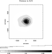
By solving the above equations we can find the cooling flow fraction in a particular band. In Band $C$ the cooling flow fraction is

$$f_{C} = \frac{N_{\mathrm{cf}}\>C_{\mathrm{cf}}}{N_{\mathrm{iso}}\>C_{\mathrm{iso}}+N_{\mathrm{cf}}\>C_{\mathrm{cf}}}$$ (8)

$$= \frac{C_{\mathrm{cf}}(C_{\mathrm{iso}}-\left[\frac{C}{D}\right]_{\mathrm{obs}}\>D_{\mathrm{iso}})}{\left[\frac{C}{D}\right]_{\mathrm{obs}}\>(D_{\mathrm{cf}}\>C_{\mathrm{iso}}-C_{\mathrm{cf}}\>D_{\mathrm{iso}})}.$$

Note that the model predictions, $X_{\mathrm{iso}}$ and $X_{\mathrm{cf}}$ are functions of metallicity, absorbing column density and temperature. We made the assumption of constant metallicity, isothermal temperature (or upper cooling temperature) and obscuration by galactic column. Those clusters with strong cooling flows show large cooling flow fractions at their centres. In Fig. 14 we present $C$ band cooling flow fraction profiles for our four example clusters. The errors shown only take account of the uncertainties in the $C/D$ ratio.

4.3 Calculating intrinsic absorption

By rearranging equations (5), (6) and (7), we can predict the observed $B/D$ colour from the $C/D$ colour and the models. Rearranging,

$$\left[\frac{B}{D}\right]_{\mathrm{pred}}=\frac{\left[\frac{C}{D}\right]_{\mathrm{obs}}-\frac{C_{\mathrm{cf}}}{D_{\mathrm{cf}}}}{\frac{C_{\mathrm{iso}}}{B_{\mathrm{iso}}}-\frac{C_{\mathrm{cf}}}{B_{\mathrm{iso}}}\frac{D_{\mathrm{iso}}}{D_{\mathrm{cf}}}}+\frac{\left[\frac{C}{D}\right]_{\mathrm{obs}}-\frac{C_{\mathrm{iso}}}{D_{\mathrm{iso}}}}{\frac{C_{\mathrm{cf}}}{B_{\mathrm{cf}}}-\frac{C_{\mathrm{iso}}}{B_{\mathrm{cf}}}\frac{D_{\mathrm{cf}}}{D_{\mathrm{iso}}}}.$$ (9)

We found that the predicted $B/D$ colour does not match the observed value. The $B/D$ ratio is more sensitive to absorption than the $C/D$ ratio (Fig. 11 and 12). Assuming the difference between the observed and predicted values of $B/D$ is due to intrinsic absorption, then it is possible to use the above equation to find the increase in absorption. We varied the obscuring column density to find $\{B,C,D\}_{\{\mathrm{iso},\mathrm{cf}\}}$ until the predicted $B/D$ ratio from equation (9) was the same as the observed one.

We then plotted a profile showing the required extra absorption above galactic as a function of contour for each cluster. Those clusters with strong cooling flows show an increase in absorption at their centres. Fig. 15 shows profiles of the required extra absorption for our example four clusters. Listed in Table 4 are the required absorption increases for each cluster in our sample. This value is the difference between the absorption in the central contour and the mean of the two outer ones. We took the mean outer contours to decrease the chance of background contamination. We looked at the difference in absorption between the centre and outside of the cluster, rather than the absolute difference from the central absorption to galactic, because the galactic absorption value is uncertain for many clusters. The errors on the values assume that all uncertainty is due to the observed $B/D$ ratio. $S(\Delta N_{H})$ shows the significance of the increased absorption using an expression with the same form as equation (3).

5 Discussion

5.1 Adaptively-smoothed images

Many of the cooling flow clusters in our sample show relatively featureless elliptical images after adaptive smoothing. We present some interesting ones, and those of the Perseus, Virgo and A2199 clusters in Fig. 1, 2 and 3. The clusters show structure which appears to vary between the different bands.

5.2 The sample of clusters

Fig. 7 and 8 show that clusters with low galactic latitude, or those masked by regions of high absorption, show low $B/D$ and $C/D$ colours. These clusters include, for example, Ophiuchus, PKS 0745-191 and Cygnus A.

Those clusters with strong cooling flows show large $C/D$ ratios, or softer X-rays, at their centres, with large $C/D$ gradients moving towards their centres. These include, for example, Virgo, Perseus, 2A 0335+096, Centaurus and A2199. They therefore contain cool gas at small radii, within a few arcminutes of the centre. This can be seen by comparison with the theoretical curves in Fig. 11. The only way of achieving the gradient is by adding cooler gas. Those clusters without strong cooling flows do not show this strong colour gradient, for example, Coma, A2256 and A119.

5.3 Comparison with models

The isothermal temperatures derived using the isothermal model in the outer regions of the clusters agree in most cases with those derived from $ASCA$ data (White 2000). There are a few clusters, most of which are absorbed by high galactic column densities, for which we find unusually low temperatures. These include Perseus, PKS 0745-191, A478 and Cygnus-A. We note that we were able to reproduce the Perseus $ASCA$ temperature result using a column of $10^{21}$ atom $\textrm{cm}^{-2}$.

Those clusters with strong cooling flows show good evidence of absorbing material at their centres. For example Virgo, Centaurus, Perseus and A478 all show significant increased levels of absorption. There is no evidence for absorbing material in those clusters without cooling flows. Abundance gradients in cooling flow clusters have been observed, for example in the Centaurus cluster (Fukazawa et al. 1994), the Virgo cluster (Matsumoto et al. 1996) and AWM7 (Ezawa et al. 1997), with the metallicities decreasing outwards from the cluster centres. Due to the relationship on $B/D$ colour from absorption and metallicity, there is some degeneracy in the two variables. At low temperatures metallicity has its strongest effect (Fig. 11), so if we have overestimated the levels of absorption, then it will be primarily for those clusters with metallicity gradients. However, we found that metallicity gradients were not sufficient by themselves to account for the observed colour gradients.

The PSPC detector limits the energy bounds of our observations. There are too few independent energy bands to make more than two colours, which limits the number of physical quantities we can fit the data. More colours will help to completely resolve any degeneracy between metallicity and absorbing column density. Data from Chandra will be able to solve this completely. The increased effective area of the telescope will also improve our statistics, reducing the uncertainties in our colours.

Allen & Fabian (1997) used a partial screening model in conjunction with a deprojection method on their data. Using a partial screening model results in larger column densities than those predicted without. Doing a similar analysis would show larger levels of absorption in our clusters, however it would add unnecessary complexity to our procedure. We also did not take the absorption results to check for consistency with the $C/D$ ratio, but do not expect the results to be significantly different.

6 Conclusions

We have presented an analysis of X-ray colour maps. The analysis technique attempts to group areas of the image together in order to maximize the signal to noise of the results, but preserving information about the structure of the object. This technique will be useful in examining data from the current generation of new X-ray telescopes. These data will show large variations in count rate, and will need analysis which is more intelligent than simple binning.

We created colour X-ray maps of the cores of a sample of 33 clusters, almost doubling the sample of Allen & Fabian (1997). The profiles generated from these maps show that there is cooling gas at the centres of those clusters with strong cooling flows. There is no evidence for cooling gas in clusters inferred from imaging deprojection or other methods to have weak, or no, cooling flow. We find a clear anti-correlation between the central cooling time of a cluster and the $C/D$ colour gradient significance. The central cooling time is an indicator of the quality of cooling flow data. We also find a correlation between the cooling flow flux and the $C/D$ significance. The maps of the non-cooling-flow clusters contain more structure as a group than those clusters with cooling flows.

We fitted a single-phase isothermal model to the $C/D$ colour of each of the contours of our sample of clusters. Those clusters with strong cooling flows show a significant decrease in the fitted temperatures of their inner contours relative to their outer contours. An isothermal gas with a varying metallicity alone was also not able to fit our data. We added a cooling flow component to the model with the same upper temperature as the isothermal plasma. Those clusters with cooling flows required the addition of a significant fraction of cooling flow model in their centres to account for the $C/D$ colour. To fit the observed $B/D$ colour we required the addition of extra absorbing material at the centres of our strong cooling flow clusters. This provides more evidence that cooling flows accumulate cold material. There was no evidence for intrinsic absorbing material for clusters without cooling flows.

References

- [1] Allen S.W., Fabian A.C., 1997, MNRAS, 286, 583
- [2] Böhringer H., Voges W., Fabian A.C., Edge A.C., Neumann D.M., 1993, MNRAS, 264, L25
- [3] Böhringer H., Nulsen P.E.J., Braun R., Fabian A.C., 1995, MNRAS, 274, L67
- [4] Dickey, J.M., Lockman F.J., 1990, ARA&A, 28, 215
- [5] Ebeling H., White D.A., Rangarajan F.V.N., MNRAS, accepted, ASMOOTH: A simple and efficient algorithm for adaptive kernel smoothing of two-dimensional imaging data
- [6] Ezawa H., Fukazawa Y., Makishima K., Ohashi T., Takahara F., Xu H., Yamasaki N.Y., 1997, ApJ, 490, L33
- [7] Fabian A.C., 1994, A&AR, 32, 277
- [8] Fukazawa Y., Ohashi T., Fabian A.C., Canizares C.R., Ikebe Y., Makishima K., Mushotzky R.F., Yamashita K., 1994, PASJ 46, L55
- [9] Liedahl, D.A., Osterheld, A.L., Goldstein, W.H., 1995, ApJ, 438, L115
- [10] Johnstone R.M., Fabian A.C., Edge A.C., Thomas P.A., 1992, MNRAS, 255, 431
- [11] Matsumoto H., Koyama K., Awaki H., Tomida H., Tsura T., Mushotzky R., Hatsukade L., 1996, PASJ, 48, 201
- [12] Mewe R., Gronenschild E.H.B.M., van den Oord G.H.J., 1985, A&AS, 62, 197
- [13] Peres C.B., Fabian A.C., Edge A.C., Allen S.W., Johnstone R.M., White D.A., 1998, MNRAS, 298, 416
- [14] Plucinsky, P.P., Snowden S.L., Briel U.G., Hasinger, G., Preffermann, E., 1993, ApJ, 418, 519
- [15] Snowden S.L., McCammon D., Burrows D.N., Mendenhall, J.A., 1994, ApJ, 424, 714
- [16] Snowden S.L., Kuntz K.D., 1998, Cookbook for ROSAT observations of extended objects, ftp://legacy.gsfc.nasa.gov/rosat/software/fortran/sxrb/esas.ps.gz
- [17] Starck J.L., Pierre M., 1998, A&AS, 128, 397
- [18] White D.A., 2000, MNRAS, 312, 663