Slow-roll inflation and CMB anisotropy data

Abstract

We emphasize that the estimation of cosmological parameters from cosmic microwave background (CMB) anisotropy data, such as the recent high resolution maps from BOOMERanG and MAXIMA-1, requires assumptions about the primordial spectra. The latter are predicted from inflation. The physically best-motivated scenario is that of slow-roll inflation. However, very often, the unphysical power-law inflation scenario is (implicitly) assumed in the CMB data analysis. We show that the predicted multipole moments differ significantly in both cases. We identify several misconceptions present in the literature (and in the way inflationary relations are often combined in popular numerical codes). For example, we do not believe that, generically, inflation predicts the relation $n_{\rm S}-1=n_{\rm T}$ for the spectral indices of scalar and tensor perturbations or that gravitational waves are negligible. We calculate the CMB multipole moments for various values of the slow-roll parameters and demonstrate that an important part of the space of parameters $(n_{\rm S},n_{\rm T})$ has been overlooked in the CMB data analysis so far.

1 Introduction

Accurate measurements of the cosmic microwave background (CMB) anisotropies provide an excellent mean to probe the physics of the early Universe, in particular the hypothesis of inflation. Recently, scientists working with the BOOMERanG (de Bernardis et al., 2000) and MAXIMA-1 (Hanany et al., 2000) CMB experiments announced the clear detection of the first acoustic peak at an angular scale $\simeq 1^{\circ}$, which confirms the most important prediction of inflation: the Universe seems to be spatially flat (Lange et al., 2000; Balbi et al., 2000).

In the framework of inflation CMB anisotropies follow from the basic principles of general relativity and quantum field theory. To predict the multipole moments of these CMB anisotropies two ingredients are necessary: the initial spectra of scalar and tensor perturbations and the “transfer functions”, which describe the evolution of the spectra since the end of inflation. The transfer functions depend on cosmological parameters such as the Hubble constant ($h$), the total energy density ($\Omega_{0}$), the density of baryons ($\Omega_{\rm b}$), the density of cold dark matter ($\Omega_{\rm cdm}$) and the cosmological constant ($\Omega_{\Lambda}$).

For the analysis of CMB maps it is a reasonable first step to test the most simple and physical model of the early Universe: slow-roll inflation with a single scalar field. Slow-roll inflation predicts a logarithmic dependence of the power spectra on the wave number $k$ (Starobinsky, 1979; Mukhanov and Chibisov, 1981; Guth and Pi, 1982; Starobinsky, 1982; Hawking, 1982). However, in most studies of the CMB anisotropy the spectral shape of power-law inflation (Abbott and Wise, 1984), corresponding to an exponential potential for the inflaton field, has been considered. This case is unphysical, since power-law inflation does never stop. Two of us (Martin and Schwarz, 2000) have shown, using analytical techniques, that the predictions of power-law and slow-roll inflation can differ significantly. Here, we confirm these results and calculate the CMB anisotropies with a full Boltzmann code developed by one of us (A. R.). The numerical accuracy of this code has been tested by comparison to analytical results (low $\ell$) and to CMBFAST v3.2 (Seljak and Zaldarriaga, 1996). In general both codes agree within $2\%$.

We use the new CMB data to test slow-roll inflation, assuming the two most popular versions of Cold Dark Matter (CDM) models (our “priors”): the standard CDM model (SCDM: $\Omega_{0}=1$, $\Omega_{\rm cdm}=1-\Omega_{\rm b}$) and the cosmic concordance model ($\Lambda$CDM: $\Omega_{0}=1$, $\Omega_{\rm\Lambda}=0.7$, $\Omega_{\rm cdm}=1-\Omega_{\rm b}-\Omega_{\rm\Lambda}$), which is motivated by the results of the high-$z$ supernovae searches (Perlmutter et al., 1998; Riess et al., 1998). In particular, we take $\Omega_{0}=1$ in agreement with the most important prediction of inflation, $h=0.60$, which is consistent with supernovae type Ia measurements [$h=0.585\pm 0.063$ at $90\%$ C.L. (Parodi et al., 2000)], and $\Omega_{\rm b}h^{2}=0.019$, as inferred from the observed abundance of D and primordial nucleosynthesis [$\Omega_{\rm b}h^{2}=0.019\pm 0.002$ (Tytler et al., 2000; Nollett and Burles, 2000)].

In this letter we recall the basic predictions of slow-roll inflation (Sec. 2) and correct errors and misconceptions that have been recently made in the literature on this issue (Sec. 3). In section 4 we compare for the first time the predictions of slow-roll inflation with the recent data of BOOMERanG and MAXIMA-1 (without any elaborated statistical technique; we remind that only $5\%$ of the BOOMERanG data have been analyzed so far).

2 Predictions of inflation

The power spectra from power-law inflation, for which the scale factor behaves as $a(\eta)\propto|\eta|^{1+\beta}$ with $\beta\leq-2$, change with a fixed power of the wavenumber $k$. For the Bardeen potential and for gravitational waves the power spectra in the matter-dominated era are respectively given by (Abbott and Wise, 1984; Martin and Schwarz, 1998)

$$k^{3}P_{\rm\Phi}=A\frac{3-n_{\rm S}}{1-n_{\rm S}}\biggl{(}\frac{k}{k_{0}}\biggr{)}^{n_{\rm S}-1},\ k^{3}P_{\rm h}=A\frac{400}{9}\biggl{(}\frac{k}{k_{0}}\biggr{)}^{n_{\rm T}},$$ (1)

where $k_{0}$ is a pivot scale and where $n_{\rm S}-1\equiv{\rm d}\ln(k^{3}P_{\rm\Phi})/{\rm d}\ln k=n_{\rm T}\equiv{\rm d}\ln(k^{3}P_{\rm h})/{\rm d}\ln k=2\beta+4$. The factor $A$ is predicted from inflation, its expression is given in Martin and Schwarz (2000). Here, $A$ is a priori free and must be tuned such that the angular spectrum is COBE-normalized. The choice of $\beta$ fixes $n_{\rm S}$ and $n_{\rm T}$ and we always have $n_{\rm S}<1$. The predictions of power-law inflation are the same for any value of the pivot scale, since $k_{0}$ can be included into the definition of $A$.

Let us now turn to slow-roll inflation which is certainly physically more relevant, since it covers a wide class of inflationary models. Slow-roll is essentially controlled by two parameters: $\epsilon\equiv-\dot{H}/H^{2}$ and $\delta\equiv-\dot{\epsilon}/(2H\epsilon)+\epsilon$, where $H$ is the Hubble rate. These two parameters can be related to the shape of the inflaton potential (Lidsey et al., 1997). All derivatives of $\epsilon$ and $\delta$ have to be negligible, e.g. $\dot{\delta}/H={\cal O}(\epsilon^{2},\epsilon\delta,\delta^{2})$, only then the slow-roll approximation is valid. Slow-roll inflation corresponds to a regime where $\epsilon$ and $|\delta|$ are constant and small in comparison with unity. The power spectra of the Bardeen potential and gravitational waves can be written as (Stewart and Lyth, 1993; Martin and Schwarz, 2000)

$$k^{3}P_{\rm\Phi} = \frac{A}{\epsilon}\biggl{[}1-2\epsilon-2(2\epsilon-\delta)\biggl{(}C+\ln\frac{k}{k_{0}}\biggr{)}\biggr{]},$$ (2)

$$k^{3}P_{\rm h} = \frac{400A}{9}\biggl{[}1-2\epsilon\biggl{(}C+1+\ln\frac{k}{k_{0}}\biggr{)}\biggr{]},$$ (3)

where $C\equiv\gamma_{\rm E}+\ln 2-2\simeq-0.7296$, $\gamma_{\rm E}\simeq 0.5772$ being the Euler constant. Slow-roll inflation predicts the value of $A$, which is given in Martin and Schwarz (2000) and has not necessarily the same numerical value as for power-law inflation. One important difference to power-law inflation is that the choice of the pivot scale $k_{0}$ now matters. It has been shown in Martin and Schwarz (2000) that the slow-roll error in the scalar multipoles is minimized at the multipole index $\ell=\ell_{\rm opt}$ if $D_{\ell_{\rm opt}}=\ln(k_{0}r_{\rm lss})$, where $r_{\rm lss}$ is the comoving distance to the last scattering surface and $D_{\ell}\equiv 1-\ln 2+\Psi(\ell)+(\ell+1/2)/[\ell(\ell+1)]$ with $\Psi(x)\equiv{\rm d}\ln\Gamma(x)/{\rm d}x$. For $\ell_{\rm opt}\gg 1$ this gives $k_{0}\simeq(e\ell_{\rm opt})/(2r_{\rm lss})$, where $r_{\rm lss}=2/(aH)_{0}$ for SCDM and $r_{\rm lss}\simeq 3.3/(aH)_{0}$ for $\Lambda$CDM. Usually the choice $k_{0}=(aH)_{0}$ is made, which corresponds to $\ell_{\rm opt}\simeq 2$. In this letter we also consider the case $\ell_{\rm opt}=200$, which roughly corresponds to the location of the first acoustic peak. Finally, from Eqs. (2) – (3) the spectral indices are inferred

$$n_{\rm S}=1-4\epsilon+2\delta,\quad n_{\rm T}=-2\epsilon.$$ (4)

An important consequence of these formulas is that the relation $n_{\rm S}=n_{\rm T}+1$ does not hold for slow-roll inflation, except in the particular case $\epsilon=\delta$.

3 CMB data analysis

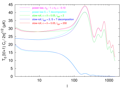
Figure 1: Comparison of CMB band powers from power-law and slow-roll inflation in the SCDM scenario. The slow-roll model has $\epsilon=\delta=0.050$ such that the scalar and tensor spectral indices agree in both cases ($n_{\rm S}=0.9$, $n_{\rm T}=-0.1$), which means for the power-law model $\epsilon=\delta\simeq 0.053$. For $\ell_{\rm opt}=2$, the usual pivot, the difference between the power-law and slow-roll spectra is large, which improves for a pivot $\ell_{\rm opt}=200$. The contribution of gravitational waves is displayed for power-law and slow-roll inflation ($\ell_{\rm opt}=2$).

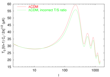
Figure 2: CMB band powers for a power-law spectrum ($n_{\rm S}=0.9$) in the $\Lambda$CDM scenario with correct (red line) and incorrect (green line) contribution of gravitational waves.

We found five misconceptions in the literature, which do have an important impact on the extraction of cosmological parameters from the measured CMB multipole moments: a- From Eqs. (1) and (2) – (3) we see that the shapes of the spectra are not the same in power-law inflation and in slow-roll inflation (even if $\epsilon=\delta$). Unfortunately, the unphysical power-law shape (1) is assumed frequently, although the relevance of deviations from the power-law shape has been discussed earlier [see e.g. Kosowsky and Turner (1995); Lidsey et al. (1997)]. This difference in the shape affects the estimates of cosmological parameters in Lange et al. (2000) and Balbi et al. (2000), since this misconception is built in into the most commonly used numerical codes: CMBFAST and CAMB (Lewis et al., 1999). In Martin and Schwarz (2000) it has been demonstrated that the difference is important and increases with $|n_{\rm S}-1|$. For instance, with the usual choice $\ell_{\rm opt}=2$, the error is $15\%$ at $\ell\simeq 200$ for $n_{\rm S}=0.9$, see Fig. 1. It has been suggested (Martin and Schwarz, 2000) to move the pivot scale to $\ell_{\rm opt}\simeq 200$, which decreases the difference from the spectral shapes. For the case considered before, the difference reduces to $\simeq 2\%$ with $\ell_{\rm opt}\simeq 200$, as can be seen in Fig. 1. For cases $\epsilon\neq\delta$ the error from the wrong shape increases [for the primordial spectra this has been studied by Grivell and Liddle (1996)]. Thus, for the accurate estimation of the cosmological parameters, one must not mistake power-law inflation for slow-roll inflation. We suggest to place the scale for which the slow-roll parameters $\epsilon$ and $\delta$ are determined in the region of the acoustic peaks, rather than in the COBE region, which decreases the error from the slow-roll approximation and one can get rid of the limitations from cosmic variance for the normalization. b- In various publications (Lange et al., 2000; Balbi et al., 2000) and codes (CMBFAST and CAMB) $n_{\rm S}\geq 1$ and $n_{\rm S}-1\neq n_{\rm T}$ are allowed in the data analysis, while working with power-law spectra (the prediction of power-law inflation). This is meaningless in the context of inflationary perturbations. For the case $n_{\rm S}=1$ the scalar amplitude is divergent and the linear approximation breaks down [see Eq. (1)]. If, nevertheless, the power–law shape is assumed, $n_{\rm S}=n_{\rm T}+1<1$ should be fulfilled. On the contrary, in slow-roll inflation, as can be checked on Eqs. (4), one can have $n_{\rm S}=1$ or $n_{\rm S}>1$, only $n_{\rm T}<0$ is compulsory. c- A third misconception is that gravitational waves are not taken into account properly. This is an important issue since a non-vanishing contribution of gravitational waves modifies the normalization and changes the height of the first acoustic peak. In Lange et al. (2000) (see the footnote [13]), it was assumed that if $n_{\rm S}>1$, there are no gravitational waves at all, a supposition in complete contradiction with the predictions of slow-roll inflation. Also, in that article, the relation $k^{3}P_{\rm h}/k^{3}P_{\rm\Phi}=-(200/9)n_{\rm T}/(1-n_{\rm T}/2)$ was used. It is valid for power-law inflation only. In Bridle et al. (2000) gravitational waves have been neglected, which restricts the analysis for their choice of $n_{\rm S}=1$ to the case $\delta=2\epsilon\ll{\cal O}(0.01)$, such that tensors contribute less than about $10\%$ of the power. d- By default in the CMBFAST and CAMB codes the contribution of gravitational waves is calculated according to the relation $C_{2}^{\rm T}/C_{2}^{\rm S}\simeq 7(1-n_{\rm S})$. Tegmark and Zaldarriaga (2000) argued, based on this relation, that power-law models with large tilt cannot explain the observed anisotropies. However, this relation is only valid for power-law inflation and the SCDM model. In particular this is no longer true when $\Lambda\neq 0$ ($\Lambda$CDM model). The reason is the so-called “late integrated Sachs-Wolfe effect”, which has been well known for a long time (Kofman and Starobinsky, 1985; Górski et al., 1992; Knox, 1995). The normalization must be performed utilizing the power spectra themselves and not the quadrupoles in order not to include an effect of the transfer function. In Fig. 2, we display the $\Lambda$CDM multipole moments (for $n_{\rm S}=0.9$) in the case where the wrong normalization is used together with the case where the normalization is correctly calculated with the help of Eqs. (2) – (3). The error is $\simeq 15\%$ at $\ell\simeq 200$. This weakens the mentioned argument of Tegmark and Zaldarriaga (2000) and in fact questions any analysis that uses the CMBFAST default scalar-tensor ratio together with a non-vanishing cosmological constant. e- Finally, CMBFAST and the pre-July 2000 versions of CAMB calculate the low-$\ell$ multipoles in the tensorial sector inaccurately. In the case of power-law inflation and the SCDM model they can be well approximated by

$$C_{\ell}^{\rm T}=\frac{9\pi}{4}(\ell-1)\ell(\ell+1)(\ell+2)A_{\ell}(n_{\rm T}),$$ (5)

with,

$$A_{\ell}(n_{\rm T})\equiv\frac{400A}{9}\int_{0}^{\infty}{{\rm d}y\over y^{1-n_{\rm T}}}\biggl{|}\int_{0}^{y}\frac{j_{2}(x)j_{\ell}(y-x)}{x(y-x)^{2}}{\rm d}x\biggr{|}^{2},$$ (6)

where $j_{\ell}$ is a spherical Bessel function. For $n_{\rm T}=0$, this gives in agreement with Grishchuk (1993): $C_{3}^{\rm T}/C_{2}^{\rm T}\simeq 0.393$. The code developed by one of us (A.R.) reproduces this value with a precision better than $1\%$, whereas CMBFAST gives $C_{3}^{\rm T}/C_{2}^{\rm T}\simeq 0.361$, i.e. an error of $\simeq 8\%$. Above $\ell=4$ both codes agree reasonably well. This problem has been fixed in the July 2000 version of CAMB.

4 Test of slow-roll inflation

We now consider the most simple and physical model for inflation (i.e. slow-roll inflation optimized with $\ell_{\rm opt}=200$) for the SCDM and $\Lambda$CDM scenarios and compare its predictions with the observational data of COBE/DMR (Bennett et al., 1996), BOOMERanG and MAXIMA-1. We demonstrate that a large region of the parameter space $(n_{\rm S},n_{\rm T})$ [or equivalently $(\epsilon,\delta)$], forbidden in the case of power-law inflation but allowed in the case of slow-roll inflation, contains models which fit the data as good as the models usually considered in the data analysis.

The data are very often presented in terms of band-power $\delta T_{\ell}^{2}\equiv T_{0}^{2}\ell(\ell+1)C_{\ell}/(2\pi)$, with $T_{0}\simeq 2.7\mbox{K}$. For any value of $\epsilon$ and $\delta$, $\delta T_{\ell}^{2}$ can be approximatively expressed in terms of the band-power for $\epsilon$, $\delta\ll 1$

$$\delta T_{\ell}^{2}(\epsilon,\delta)\simeq\frac{\delta T_{\ell}^{2}(\epsilon,\delta\ll 1)}{1+R_{10}}\biggl{[}1-2(2\epsilon-\delta)\ln\frac{\ell}{10}\biggr{]}.$$ (7)

A corresponding formula for power-law inflation has been presented in Turner et al. (1993) [see remark before Eq. (33)]. For the SCDM and $\Lambda$CDM scenarios considered here (see the introduction), we have respectively for the first peak: $\delta T_{207}^{2}(\epsilon,\delta\ll 1)\simeq 3705(\mu\mbox{K})^{2}$, $\delta T_{222}^{2}(\epsilon,\delta\ll 1)\simeq 6422(\mu\mbox{K})^{2}$, and for the second peak $\delta T_{497}^{2}(\epsilon,\delta\ll 1)\simeq 1952(\mu\mbox{K})^{2}$, $\delta T_{565}^{2}(\epsilon,\delta\ll 1)\simeq 3102(\mu\mbox{K})^{2}$. In the previous equation, we have assumed $\delta T_{\ell}^{2}(\epsilon,\delta)\simeq\delta T_{\ell}^{{\rm S}\,2}(\epsilon,\delta)$ which is valid only if $\ell\gg 1$ in order for the tensorial modes to be negligible. The quantity $R_{10}$ is defined by $R_{10}\equiv\delta T_{10}^{{\rm T}\,2}/\delta T_{10}^{{\rm S}\,2}$ and appears because the spectrum is normalized to the multipole $C_{10}$. At the leading order, it can be expressed as $R_{10}\simeq-5.31n_{\rm T}$ and at the next-to-leading order, it is given by

$$R_{10}=10.62\epsilon[1+3.96\epsilon-3.85\delta-2(\epsilon-\delta)\ln(100e)].$$ (8)

Eq. (7) permits us to roughly understand how the spectrum is modified when the slow-roll parameters are changed. For fixed $2\epsilon-\delta$, i.e. for a fixed scalar spectral index $n_{\rm S}$, increasing $\epsilon$, i.e. increasing the value of $n_{\rm T}$, lowers $\delta T_{\ell}^{2}$. Increasing $2\epsilon-\delta$ (i.e. decreasing $n_{\rm S}$) while $\epsilon$ (i.e. $n_{\rm T}$) remains constant has the same effect.

In Figs. 3 (SCDM scenario) and 4 ($\Lambda$CDM scenario), we display the theoretical predictions of slow-roll inflation for some values of the slow-roll parameters. Without performing a $\chi^{2}$-analysis, our main conclusion is that there exist models that reasonably fit available CMB data, which were not included in the estimates of cosmological parameters before, in particular in the data analysis of the recent CMB maps (Lange et al., 2000; Balbi et al., 2000). This includes models with $n_{\rm S}-1\neq n_{\rm T}$ and non-negligible gravitational waves contribution. For instance, the model $\epsilon=0.02$, $\delta=0.04$ (i.e. $n_{\rm S}=1$ and $n_{\rm T}=-0.04$) in the $\Lambda$CDM scenario, see Fig. 4 goes through all the MAXIMA-1 data points (at 1$\sigma$) but one. In this particular case, gravitational waves represent $33\%$ of the power at $\ell=2$, i.e. $R_{2}=0.33$. This provides a good example which violates common (unjustified) believes about inflation. Let us stress that for both figures we did not optimize the fits by exploring the $10\%$ resp. $4\%$ uncertainty in the calibration of the BOOMERanG and MAXIMA-1 results, nor did we optimize the fits by varying $h$ and $\Omega_{\rm b}h^{2}$ nor any other parameters.

5 Conclusion

It is impossible to extract the values of cosmological parameters from the CMB anisotropy data without assumptions on the initial spectra. For this purpose, slow-roll inflation is the best model presently known and is consistent with presently available data. Unfortunately, very often, only power-law inflation is considered. The difference between both models is in general significant, which implies that only a limited part of the space of parameters has been correctly studied so far. Data analysis has been based on unjustified prejudices that $n_{\rm S}$ may be greater than one in power-law inflation, that the relation $n_{\rm S}-1=n_{\rm T}$ must hold in general and that, gravitational waves are negligible in general. We want to stress that a subdominant effect (as the contribution of gravitational waves in many inflation models) is not necessarily negligible. Although very important on the conceptual side, the previous misconceptions were not crucial for the COBE/DMR experiment. For the next generation of measurements, which aim to extract cosmological parameters with a precision of a few percent, distinguishing power-law inflation from slow-roll inflation becomes mandatory. We think that a correct analysis of the CMB data should start from the spectra given in Eqs. (2)–(3) and should be performed in the whole space of parameters ($0<\epsilon\ll 1,|\delta|\ll 1)$. This should result in the determination of the best $\epsilon$ and $\delta$. The present letter hopefully motivates more detailed tests of the most simple inflationary scenario: slow-roll inflation.

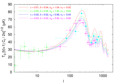
Figure 3: CMB band powers for slow-roll inflation in the SCDM scenario for different values of the slow-roll parameters together with the data points of the COBE/DMR (crosses), BOOMERanG (open boxes) and MAXIMA-1 (filled boxes) experiments.

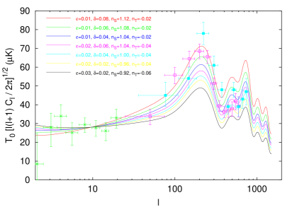
Figure 4: As Fig. 3 but for the $\Lambda$CDM scenario.

References

- Abbott and Wise (1984) Abbott, L. F., and Wise, M. B. 1984, Nucl. Phys. B244, 541
- Balbi et al. (2000) Balbi, A., et al. 2000, astro-ph/0005124
- Bennett et al. (1996) Bennett, C. L. et al. 1996, ApJ, 464, L1
- Bridle et al. (2000) Bridle, S. L., et al. 2000, astro-ph/0006170
- de Bernardis et al. (2000) de Bernardis, P., et al. 2000, Nature, 404, 955
- Górski et al. (1992) Górski, K. M., Silk, J., and Vittorio, N. 1992, Phys. Rev. Lett., 68, 733
- Grishchuk (1993) Grishchuk, L. P. 1993, Phys. Rev. D, 48, 3513
- Grivell and Liddle (1996) Grivell, I. J., and Liddle, A. R. 1996, Phys. Rev. D, 54, 7191
- Guth and Pi (1982) Guth, A., and Pi, S. Y. 1982, Phys. Rev. Lett., 49, 1110
- Hanany et al. (2000) Hanany, S., et al. 2000, astro-ph/0005123
- Hawking (1982) Hawking, S. 1982, Phys. Lett., 115B, 295
- Knox (1995) Knox, L. 1995, Phys. Rev. D, 52, 4307
- Kofman and Starobinsky (1985) Kofman, L. A., and Starobinsky, A. A. 1985, Sov. Astron. Lett., 11, 271
- Kosowsky and Turner (1995) Kosowsky, A., and Turner, M. S. 1995, Phys. Rev. D, 52, R1739
- Lange et al. (2000) Lange, A. E., et al. 2000, astro-ph/0005004
- Lewis et al. (1999) Lewis, A., Challinor, A., and Lasenby, A. 1999, astro-ph/9911177; http://www.mrao.cam.ac.uk/~aml1005/cmb/
- Lidsey et al. (1997) Lidsey, J. E., et al. 1997, Rev. Mod. Phys., 69, 373
- Martin and Schwarz (1998) Martin, J., and Schwarz, D. J. 1998, Phys. Rev. D, 57, 3302
- Martin and Schwarz (2000) Martin, J., and Schwarz, D. J. 2000, Phys. Rev. D, 62, 103520
- Mukhanov and Chibisov (1981) Mukhanov, V., and Chibisov, G. 1981, JETP Lett., 33, 532
- Nollett and Burles (2000) Nollett, K. M., and Burles, S. 2000, astro-ph/0001440
- Parodi et al. (2000) Parodi, B. R., et al. 2000, ApJ, 540, 634
- Perlmutter et al. (1998) Perlmutter, S., et al. 1998, Nature, 391, 51
- Riess et al. (1998) Riess, A. G., et al. 1998, AJ, 116, 1009
- Seljak and Zaldarriaga (1996) Seljak, U., and Zaldarriaga, M. 1996, ApJ, 469, 437; http://www.sns.ias.edu/~matiasz/CMBFAST/cmbfast.html
- Starobinsky (1979) Starobinsky, A. A. 1979, JETP Lett., 30, 682
- Starobinsky (1982) Starobinsky, A. A. 1982, Phys. Lett., 117B, 175
- Stewart and Lyth (1993) Stewart, E. D., and Lyth, D. H. 1993, Phys. Lett., 302B, 171
- Tegmark and Zaldarriaga (2000) Tegmark, M., and Zaldarriaga, M. 2000, Phys. Rev. Lett., 85, 2240
- Turner et al. (1993) Turner, M. S., White, M., and Lidsey, J. E. 1993, Phys. Rev. D, 48, 4613
- Tytler et al. (2000) Tytler, D., et al. 2000, Phys. Scr., T85, 12