An ISOCAM absorption survey of the structure of pre-stellar cloud cores

Abstract

We present the results of a mid-infrared ($\lambda\simeq$ 7 $\mu$m) imaging survey of a sample of 24 starless dense cores carried out at an angular resolution of 6$\arcsec$ with the ISOCAM camera aboard the Infrared Space Observatory (ISO). The targeted cores are believed to be pre-stellar in nature and to represent the initial conditions of low-mass, isolated star formation. In previous submillimeter dust continuum studies of such pre-stellar cores, it was found that the derived column density profiles did not follow a single power-law such as $N_{H_{2}}\propto\bar{r}^{-1}$ throughout their full extent but flattened out near their center. These submillimeter observations however could not constrain the density profiles at radii greater than $\sim$ 10000 AU. The present absorption study uses ISOCAM’s sensitivity to map these pre-stellar cores in absorption against the diffuse mid-infrared background. The goal was to determine their structure at radii that extend beyond the limits of sensitivity of the submillimeter continuum maps and at twice as good an angular resolution. Among the 24 cores observed in our survey, a majority of them show deep absorption features. The starless cores studied here all show a column density profile that flattens in the center, which confirms the submillimeter emission results. Moreover, beyond a radius of $\sim 5000-10000$ AU, the typical column density profile steepens with distance from core center and gets steeper than $N_{H_{2}}\propto\bar{r}^{-1}$, until it eventually merges with the low-density ambient molecular cloud. At least three of the cores present sharp edges at $R\sim 15000-30000$ AU and appear to be decoupled from their parent clouds, providing finite reservoirs of mass for subsequent star formation.

1 Introduction

Although our general understanding of low-mass star formation has made significant theoretical and observational progress in the past three decades (see, e.g., the volumes by Levy & Lunine 1993 and Mannings, Boss, & Russell 2000 for comprehensive reviews), the earliest stages of the star formation process remain poorly known. These stages immediately preceding and immediately following the onset of protostellar collapse are of great interest since to some extent they must govern the origin of stellar masses, i.e., the stellar initial mass function.

According to present ideas on isolated star formation (e.g. Shu, Adams, & Lizano 1987), the first evolutionary phase in the path from molecular cloud to main sequence star involves the formation of gravitationally-bound, starless dense cores (e.g. Myers 1999). These “pre-protostellar” (or “pre-stellar” for brevity) cores (cf. Ward-Thompson et al. 1994) are thought to be initially supported against their self-gravity by magnetic and/or turbulent pressure, and to progressively evolve toward higher degrees of central concentration through ambipolar diffusion (e.g. Mouschovias 1991) and/or the dissipation of turbulence (e.g. Nakano 1998). At some not yet well understood point, the cores become unstable and collapse dynamically to form accreting protostars which quickly become detectable in the radio range as Class 0 objects (André, Ward-Thompson, & Barsony 1993) and subsequently in the infrared as Class I sources (eg. Lada 1987). Additional complications arise in regions of multiple star formation (such as the $\rho$ Ophiuchi central cloud) where external triggers rather than self-initiated ambipolar diffusion may be responsible for cloud fragmentation and core formation (e.g. Loren & Wootten 1986; Boss 1995; Whitworth et al. 1996; Motte, André, & Neri 1998 – hereafter MAN98).

A good knowledge of the initial conditions for rapid protostellar collapse in star-forming cores is crucial to get at a proper theoretical description of early protostar evolution. In particular, recent studies show that the mass-infall rate during the protostellar phase is quite sensitive to the core radial density profile at the onset of dynamical collapse. When the initial density profile is flatter than $\rho\propto r^{-2}$ near core center, then the mass-infall rate is expected to feature a strong initial peak, followed by a sharp decline, at the beginning of the main accretion phase (e.g. Foster & Chevalier 1993; Henriksen, André, & Bontemps 1997). The outer core density profile also plays a fundamental role by determining whether the mass reservoir ultimately available for star formation is effectively finite or infinite. If the radial density profile approaches $\rho\propto r^{-2}$ up to large radii as in the standard paradigm of isolated star formation (Shu et al. 1987), then the mass reservoir is much larger than a typical stellar mass and feedback processes such as outflow/inflow interactions (e.g. Velusamy & Langer 1998) must eventually stop accretion onto the central protostar. On the other hand, if the initial core density profile becomes steeper than $\rho\propto r^{-3}$ beyond some finite radius, then the mass reservoir is limited and the mass accretion rate will naturally drop to negligible values after some time. In this case, the final stellar mass may be essentially determined at the pre-collapse stage.

Direct observational constraints on the radial density structure at the onset of protostellar collapse have been obtained through (sub)millimeter dust continuum mapping of a large number of starless cores and Class 0/Class I protostellar envelopes with the JCMT and IRAM 30 m telescopes (e.g. Ward-Thompson et al. 1994; André, Ward-Thompson, & Motte 1996 – hereafter AWM96; Ward-Thompson, Motte, & André 1999 – hereafter WMA99). General trends have been found: while protostellar envelopes are always highly centrally condensed, with radial density profiles consistent with $\rho\propto r^{-1.5}$ or $\rho\propto r^{-2}$ (e.g. Ladd et al. 1991, Motte & André 1999), starless cores have radial profiles that flatten out near their centers and become much flatter than $\rho\propto r^{-2}$ at radii less than a few thousand AUs (see André, Ward-Thompson, & Barsony 2000 for a review). It is however necessary to bear in mind the limitations of (sub)millimeter continuum emission maps: since the dust emission from the outer parts of cores is intrinsically very weak, (sub)millimeter mapping is mostly sensitive to the inner density structure of starless cores. The outer density structure of cores and the possible presence of edges are difficult to constrain from (sub)millimeter observations. Fortunately, starless cores can also be studied in absorption at mid-IR wavelengths (e.g. Abergel et al. 1996, Egan et al. 1998), and this technique turns out to be more sensitive to the outer parts of cores. Another advantage of the mid-IR absorption technique over (sub)millimeter emission mapping is that the column density structure of the absorbing material may be derived without any assumption about the dust temperature distribution.

In order to gain further, independent insight into cloud core structure prior to protostar formation, we undertook dedicated mid-IR imaging observations toward a broad sample of starless dense cores with the ISOCAM mid-IR camera aboard the Infrared Space Observatory (ISO). The present paper discusses the results of this mid-IR imaging program, whose immediate goal was to detect the sample cores in absorption against the diffuse mid-IR background produced by the mean galactic interstellar radiation field (e.g. Mathis, Mezger & Panagia 1983) and/or arising from the envelopes of the parent molecular clouds (e.g. Bernard et al. 1993).

The layout of the paper is as follows. In Sect. 2, we give the properties of the core sample and explain observational details. In Sect. 3, we show our ISOCAM absorption maps and analyze the associated absorption profiles in terms of column density structure. In Sect. 4, we compare our results with various theoretical models of core structure and discuss possible implications for our understanding of the pre-stellar stage of star formation. Our main conclusions are summarized in Sect. 5.

2 Observations and Data Reduction

2.1 Starless core sample

The 24 starless fields of the present survey were selected from various dark cloud and nebula catalogs (e.g. Parker 1988, Benson & Myers 1989, Bourke, Hyland & Robinson 1995, Schneider & Elmegreen 1979), on the grounds that they contained no IRAS point sources associated with a young stellar object and had an estimated mid-infrared (mid-IR) background stronger than $\sim 1$ MJy/sr at $\sim$ 7 $\mu$m. We also included a map of the dark cloud Oph D (also called L1696A) situated in the $\rho$ Ophiuchi complex, and already observed in absorption by ISOCAM (Abergel et al. 1998). The background at 7 $\mu$m was originally estimated from IRAS images, as were the 7 $\mu$m flux densities of the IRAS sources appearing in the fields. Fields containing IRAS point sources with estimated flux densities larger than 1.5 Jy at 7.75 $\mu$m (LW6 filter [7-8.5 $\mu$m]) or larger than 0.7 Jy at 6.75 $\mu$m (LW2 filter [5-8.5 $\mu$m]) had to be shifted away from the sources and/or the integration time had to be shortened in order to avoid saturating the ISOCAM detectors (see 2.2 below). The selected regions span a wide range of properties (e.g. morphologies, environments), but are all located in nearby molecular cloud complexes (distance $\leq$ 500 pc) either actively forming stars or supposed to be future hosts of star-formation activity.

Table 1: List of starless cores observed with ISOCAM

Source	R.A.(2000)	Dec. (2000)	Dist.	Filter	Map RMS	$<$I${}_{MIR}>$	I${}_{zodi}^{\ddagger}$	Absorp.	References
								Contrast
			(pc)		(MJy/sr)	(MJy/sr)	(MJy/sr)	(%)
L1517B∗	04h55m05$\aas@@fstack{s}$2	30$\degr$38$\arcmin$39$\arcsec$	140	LW2	0.07	4.4	3.8	5	(4),(6),(13)
L1512∗	05h04m09$\aas@@fstack{s}$7	32$\degr$43$\arcmin$09$\arcsec$	140	LW6	0.15	12.4	-	3	(4),(5),(6),(11),(15)
L1544∗	05h04m18$\aas@@fstack{s}$1	25$\degr$11$\arcmin$08$\arcsec$	140	LW2	0.05	4.8	4.2	8	(4),(11),(14),(15),(16)
L1582A	05h32m03$\aas@@fstack{s}$0	12$\degr$30$\arcmin$16$\arcsec$	400	LW2	0.16	8.6	3.7	44	(4),(6)
L1672	05h54m24$\aas@@fstack{s}$0	01$\degr$58$\arcmin$53$\arcsec$	200	LW2	0.19	4.7	3.4	31	(10)
BHR78	12h36m18$\aas@@fstack{s}$7	$-$63$\degr$12$\arcmin$37$\arcsec$	200	LW6	0.61	17.2	-	11	(3)
BHR111	15h42m19$\aas@@fstack{s}$7	$-$52$\degr$47$\arcmin$54$\arcsec$	250	LW6	0.41	19.5	10.0	6	(3)
R7∗∗	16h21m45$\aas@@fstack{s}$9	$-$23$\degr$42$\arcmin$51$\arcsec$	160	LW6	0.92	-	-	-	(8)
OphD∗∗	16h28m30$\aas@@fstack{s}$4	$-$24$\degr$18$\arcmin$29$\arcsec$	160	LW2†	0.3	14.8	5.7	28	(1),(8),(9)
R53∗∗	16h31m44$\aas@@fstack{s}$1	$-$24$\degr$48$\arcmin$12$\arcsec$	160	LW2	0.2	11.4	-	20	(8)
SA187	16h32m17$\aas@@fstack{s}$2	$-$44$\degr$53$\arcmin$40$\arcsec$	200	LW6	0.92	-	-	6	(12)
L1709A∗∗	16h32m42$\aas@@fstack{s}$1	$-$23$\degr$54$\arcmin$09$\arcsec$	160	LW2	0.17	12.8	10.5	17	(4),(6),(8),(11)
R60∗∗	16h33m11$\aas@@fstack{s}$8	$-$24$\degr$41$\arcmin$30$\arcsec$	160	LW2	0.13	10.1	-	7	(8)
L1709C∗∗	16h33m53$\aas@@fstack{s}$4	$-$23$\degr$42$\arcmin$32$\arcsec$	160	LW2	0.10	8.2	-	16	(4),(6),(8),(11)
R63∗∗	16h33m58$\aas@@fstack{s}$3	$-$24$\degr$30$\arcmin$03$\arcsec$	160	LW2	0.14	9.3	5.0	16	(8)
L1689B∗∗	16h34m40$\aas@@fstack{s}$1	$-$24$\degr$37$\arcmin$00$\arcsec$	160	LW2	0.05	8.3	4.3	19	(2),(4),(8),(11),(15)
L204B	16h47m32$\aas@@fstack{s}$0	$-$11$\degr$59$\arcmin$15$\arcsec$	170	LW2	0.11	15.7	-	4	(4),(11)
B68	17h22m34$\aas@@fstack{s}$7	$-$23$\degr$47$\arcmin$50$\arcsec$	200	LW2	0.19	11.5	8.8	2	(4),(10)
BHR140	17h22m53$\aas@@fstack{s}$9	$-$43$\degr$22$\arcmin$13$\arcsec$	400	LW6	0.34	10.2	6.8	9	(3)
L310	18h07m11$\aas@@fstack{s}$9	$-$18$\degr$21$\arcmin$35$\arcsec$	200	LW6	0.54	30.0	7.1	39	(11)
L328	18h17m00$\aas@@fstack{s}$4	$-$18$\degr$01$\arcmin$52$\arcsec$	200	LW6	0.7	42.9	7.4	40	(11)
L429	18h17m06$\aas@@fstack{s}$4	$-$08$\degr$15$\arcmin$51$\arcsec$	200	LW6	0.2	8.6	6.8	17	(11)
GF5	18h39m16$\aas@@fstack{s}$4	$-$06$\degr$38$\arcmin$15$\arcsec$	200	LW6	2.0	75.2	7.2	30	(13)
B133	19h09m08$\aas@@fstack{s}$8	$-$06$\degr$53$\arcmin$20$\arcsec$	400	LW6	0.13	7.9	-	3	(4),(7)

(1)=Abergel et al. 1996; (2)=AWM96; (3)=Bourke, Hyland & Robinson 1995; (4)=Benson & Myers 1989; (5)=Caselli, Myers, Thaddeus 1995; (6)=Hilton & Lahulla 1995; (7)=Keene 1981; (8)=Loren 1989; (9)=Loren et al. 1990; (10)=Leung, Kutner & Mead 1982; (11)=Parker 1988; (12)=Sandqvist & Lindroos 1976, Sandqvist 1977; (13)=Schneider & Elmegreen 1979; (14)=Tafalla et al. 1998; (15)=Ward-Thompson et al. 1994; (16)=Williams et al. 1999

^†Oph D was also mapped in the LW3, LW6 and LW9 filters (see text and Fig. 1cd). The zodiacal intensity is 45 MJy/sr in LW3.

^‡Values of I_zodi come from the zodiacal light model of Kelsall et al. (1998). Typical uncertainty is $\sim$ 20%.

^∗Cores belonging to Taurus molecular complex.

^∗∗Cores belonging to $\rho$ Ophiuchi molecular complex.

The properties of the observed cloud cores are summarized in Table 1. Column 1 lists the names of the sources as found in the dark cloud catalogues, columns 2 and 3 list the J2000 coordinates of the centre of the ISOCAM field. The image centres are sometimes shifted from their original positions as given in the dark cloud catalogues (see above). Column 4 gives the distances to the clouds. For the clouds not belonging to the $\rho$ Ophiuchi (adopted distance d = 160 pc) and Taurus (d = 140 pc) molecular complexes, we used the values from the study of Hilton & Lahulla (1995) or the results of Dame et al. (1987) on the locations of the major (giant) molecular clouds in the Galaxy to give an estimate of the distances by relating the cores to known molecular complexes according to their galactic coordinates. Column 5 gives the ISOCAM filter(s) we used for the observations of each core. Column 7 lists the mean mid-IR intensity measured off the absorption features. Included in the values listed in column 7 is the zodiacal light emission (given in Column 8). Column 9 lists the relative contrast between the intensity of the main absorption feature and the mean mid-IR intensity (column 7), in percentage of the mean mid-IR intensity .

Finally, column 10 gives the references of the dark cloud catalogues, from which our fields were selected, as well as the references of a few studies containing interesting information on the sources. From Table 1, it can be seen that the majority of the fields we observed contain absorption features. Figure 1 shows eleven cores with deep absorption (i.e., L1544, L1582A, Oph D, R53, L1709A, R63, L1689B, L310, L328, L429, GF5 – see Section 3.1)).

2.2 ISOCAM observations

2.2.1 Observational parameters

The dense cores were mapped between April 1997 and March 1998 using the LW2 (5–8.5 $\mu$m) and LW6 (7–8.5 $\mu$m) filters of ISOCAM (Cesarsky et al. 1996), the spectro-imager aboard ISO (Kessler et al. 1996), centered at 6.75 $\mu$m and 7.75 $\mu$m respectively (except for Oph D, see below). These wavelengths approximately correspond to a minimum in the dust extinction curve (see the model of Draine & Lee 1984 for diffuse clouds), providing a good opportunity to peer deep inside dark clouds. We used a pixel field of view of 6$\arcsec$, which also roughly corresponds to the FWHM size of the ISOCAM point spread function (PSF) at $\sim$ 7 $\mu$m. For a “standard” observation, an area of $10.7\arcmin\times 11\arcmin$ was covered for each core with a raster map of $6\times 4$ images and an overlap of 17 pixels in right ascension and of 6 pixels in declination. At each raster position, about 18 single read-outs were taken with an integration time per read-out of 2.1s. About 50 stabilisation read-outs had to be added at the beginning of each observation to allow the detectors to lose memory of the previous observation. For a few dense cores (L1672, SA187, and GF5), the field contained strong IRAS point sources and a shorter (0.28s) integration time per read-out was adopted in order to avoid saturation on the camera detectors. In these cases, the number of read-outs was 44 at each raster position and the total area mapped was $19.7\arcmin\times 18.8\arcmin$ for L1672 and SA187. In addition to the existing LW2 (5–8.5 $\mu$m) and LW3 (12–18 $\mu$m) maps of Abergel et al. (1996, 1998) with 6$\arcsec$ pixels, we took two new images of Oph D in the filters LW6 (7–8.5 $\mu$m) and LW9 (14–16 $\mu$m) with a pixel field of view of 3$\arcsec$. The Oph D field was covered by a raster of $6\times 3$ images with an overlap of 22 pixels in both directions. The raster was tilted by 20$\degr$ with respect to the Celestial North in order to follow the core’s elongation (see Fig. 2d of MAN98 and Fig. 1 of Abergel et al. 1998). For these images of Oph D, 15 exposures were taken at each raster position with an integration time of 10 sec per read-out. The total area covered was $2.6\arcmin\times 4.1\arcmin$.

2.2.2 Data reduction

The data were reduced using the CIA (CAM Interactive Analysis) software package. First, glitches due to cosmic rays were removed using a spatial and temporal filtering algorithm (Starck et al. 1999), then a dark current image was subtracted from all the frames. Because of the time lag in the response of the detectors, transient effects had to be corrected for. For this purpose, we used the algorithm developed by Abergel et al. (1996). Finally, the images were divided by a flatfield image to correct for the non-uniform response of the detectors over the array. Most images were made up of over 500 frames that covered a large surface area. This enabled us to use a median image of all the frames as a flatfield image. Flatfielding is here a critical operation as we are looking for intensity variations in dark objects and any flux mismatch between two contiguous raster images appears as a step in an intensity profile. Additional pixels had to be masked where the trails of glitches still affected the response of the detectors or induced a downward step in the flux level.

2.2.3 Noise estimation

In order to estimate the rms noise levels in our final images, we first derived the rms level of the temporal fluctuations for each pixel of a given raster map, taking into account the overlap of the individual raster frames (each sky position in the map was observed on average in two independent individual frames). The resulting average rms noise per pixel depends on the level of the diffuse mid-IR emission in the raster, and thus varies from core to core. Typical values are $\sim$ 0.05 MJy/sr for regions with low mid-IR background (e.g. Taurus, Eastern part of the $\rho$ Oph complex) and $\sim$ 0.1 MJy/sr for regions with high mid-IR background (e.g. L328 and L310). This temporal rms noise however does not take flatfield noise (estimated to be $\sim$ 5%) into account and could be underestimating the total amount of noise. Another approach to estimating the noise in an image is by calculating the rms noise level of the spatial fluctuations over regions showing very little structure. By doing so, we a priori overestimate the noise level since we do not discriminate between true instrumental noise in the image and small-scale spatial structure in the (emitting and/or absorbing) source. The rms values listed in Table 1 and the error bars used in the profiles of Sect. 3.4 below correspond to such spatial estimates and should thus be taken as upper limits. Note that in the densest areas, we can distinguish between small-scale structure and instrumental noise or mid-IR emission fluctuations by checking for the presence on small scales of cold, IR-absorbing condensations in high-resolution millimeter continuum maps (see 2.3 below).

2.3 Millimeter observations

In order to check that the dark patches seen in the ISOCAM images (see Fig. 1) were actually due to the presence of cold absorbing dense cores/condensations, and not to small-scale fluctuations of the mid-IR background and/or foreground, we carried out 1.3 mm continuum observations of a selected subset of our fields (see Table 2). We used the IRAM 30 m telescope equipped with the 37-channel MPIfR bolometer array in March 1998 and March/April 1999 to map the 1.3 mm dust emission of those fields that presented clear and compact absorption-like features in the ISOCAM images. On-the-fly 1.3 mm maps were taken in the dual-beam raster mode with a scanning velocity of 4$\arcsec$/sec, a spatial sampling of 2$\arcsec$ in azimuth and 4$\arcsec$ in elevation, and a chopping frequency of 2 Hz. The chop throw was set to 60$\arcsec$ for maps larger than 300$\arcsec$ and 45$\arcsec$ for smaller maps. The (FWHM) beam size of the telescope was measured to be approximately 11$\arcsec$-12$\arcsec$ on maps of Uranus. The zenith atmospheric optical depth, monitored by ‘skydips’ every 1-2 hours, was between $\sim$ 0.15 and $\sim$ 0.5. The final co-added maps are about 7$\arcmin\times 7\arcmin$ in size and consist of $\sim$ 5–6 individual coverages taken at different hour angles to improve the reconstruction technique. The data were reduced with the IRAM software for bolometer arrays (”NIC”; cf. Broguière, Neri & Sievers 1995), which uses the EKH restoration algorithm (Emerson, Klein, & Haslam 1979). The typical rms noise was $\sim$ 8 mJy/11$\arcsec$beam.

The same dense cores listed in Table 2 were also observed in the C¹⁸O(1-0) molecular line at the IRAM 30 m telescope, in order to obtain estimates of the column density in the outer parts of the cores. We used the position switching mode along cuts of about 10$\arcmin$ length sampled every 20$\arcsec$ through each of the cores, and oriented along and perpendicular to the axis of the core. The OFF position, which was checked to be free of emission, was typically taken between 15$\arcmin$ and 30$\arcmin$ away from the nominal source position. Our goal was to get good signal-to-noise ratio in the outer parts of the core in order to estimate the H₂ column density, $N_{H_{2}}$, as far from the core centre as possible (typically $\sim$ 200$\arcsec$). The total (ON+OFF) integration time was 2 minutes on average and up to 10 or 25 minutes in the outer parts of the cores in order to reach an rms sensitivity better than $\sim$ 0.1 K km s^-1. The spectral resolution was 20 kHz and the observing frequency 109 GHz. Additional N₂H⁺(1-0), H₂CO(2-1), and DCO⁺(2-1) spectra were taken at a few positions for selected cores.

During these continuum and line runs at the 30 m telescope, the pointing, as well as the focus, was checked every $\sim$ 1 hour and found to be better than $\sim 5\arcsec$ in both azimuth and elevation.

3 Results and analysis

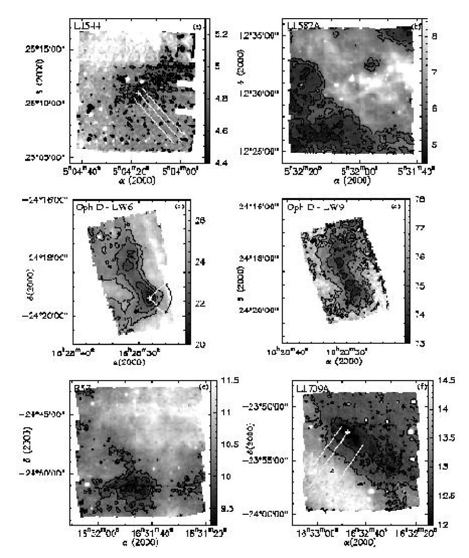
Figure 1: ISOCAM images of the sample of 11 dense cores presenting strong absorption features (see text). The cores appear as dark patches against a brighter background emission. The ISOCAM psf is $\sim$ 6$\arcsec$ (FWHM) at $\sim$ 7 $\mu$m; the pixel size is also 6$\arcsec$ (3$\arcsec$ in the case of Oph D). White crosses and triangles show the core centers and positions where the C¹⁸O column density was measured (section 3.3.2), respectively. The dotted lines/sectors illustrate the way averages were performed (section 3.4). The greyscale is indicated in MJy/sr at the right of each image. Contour levels are: a) for L1544, 4.55, 4.65, 4.75 MJy/sr; b) for L1582A, 5, 5.5, 6 MJy/sr; c) for Oph D LW6 (7.75 $\mu$m), 21, 22, 23, 24 MJy/sr; d) for Oph D LW9 (15 $\mu$m), 74, 75, 76 MJy/sr; e) for R53, 9.5, 9.75, 10 MJy/sr; f) for L1709A, 24, 25, 26 MJy/sr.

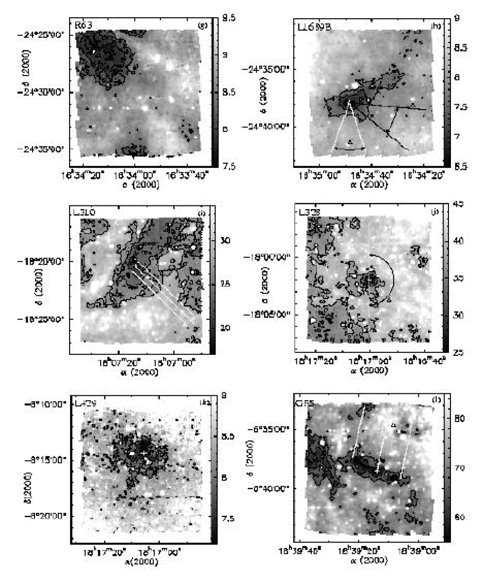
Figure 1: (cont’d) Contour levels: g) for R63, 7.75, 8, 8.25 MJy/sr; h) for L1689B, 7, 7.5, 8 MJy/sr; i) for L310, 20, 22.5, 25, 27.5 MJy/sr; j) for L328, 30, 34, 38 MJy/sr; k) for L429, 7.3, 7.7, 8.1, 8.5 MJy/sr; l) for GF5, 57, 62, 67 MJy/sr.

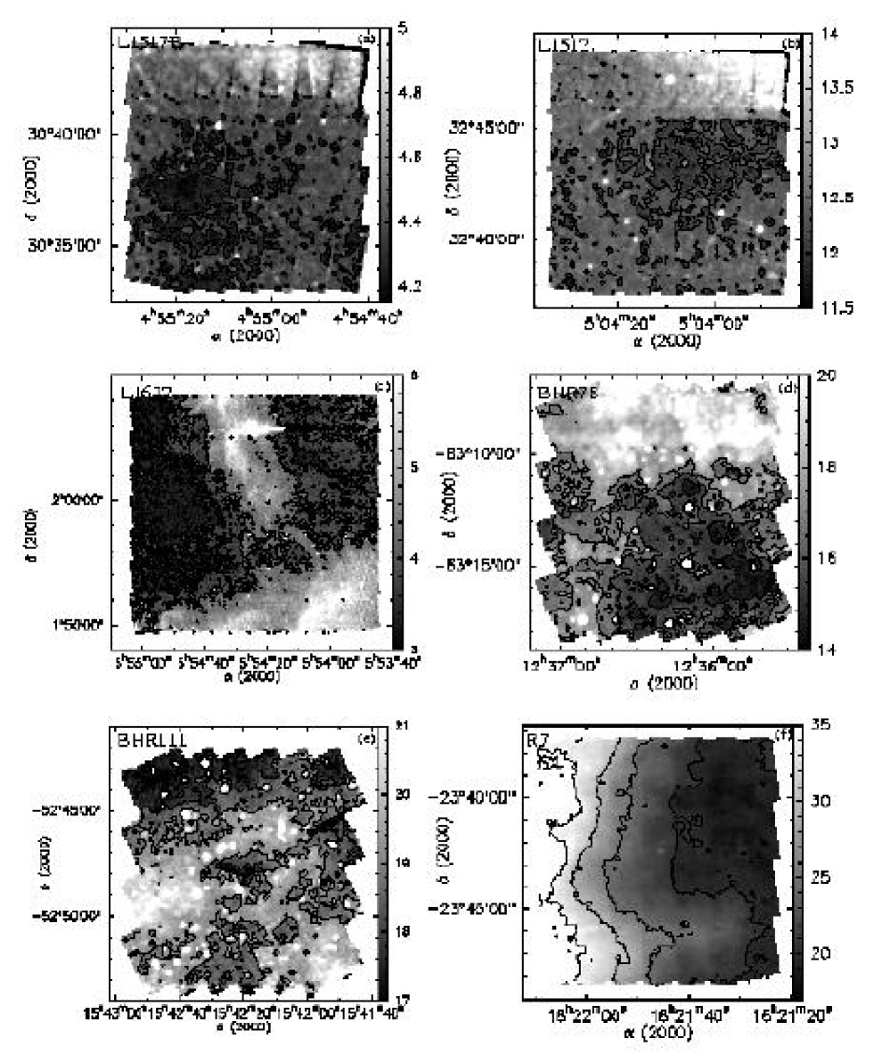
Figure 2: ISOCAM images of the remaining cores. The fainter absorption features led us to enhance the contrast of the images, which resulted in poorer image appearance (the flatfield noise is clearly visible in some cases). Contour levels are: a) for L1517B, 4.3 MJy/sr; b) for L1512, 12.2 MJy/sr; c) for L1672, 3.5, 4 MJy/sr; d) for BHR78, 15, 16, 17; e) for BHR111, 17, 18, 19 MJy/sr; f) for R7, 20, 25, 30, 35 MJy/sr.

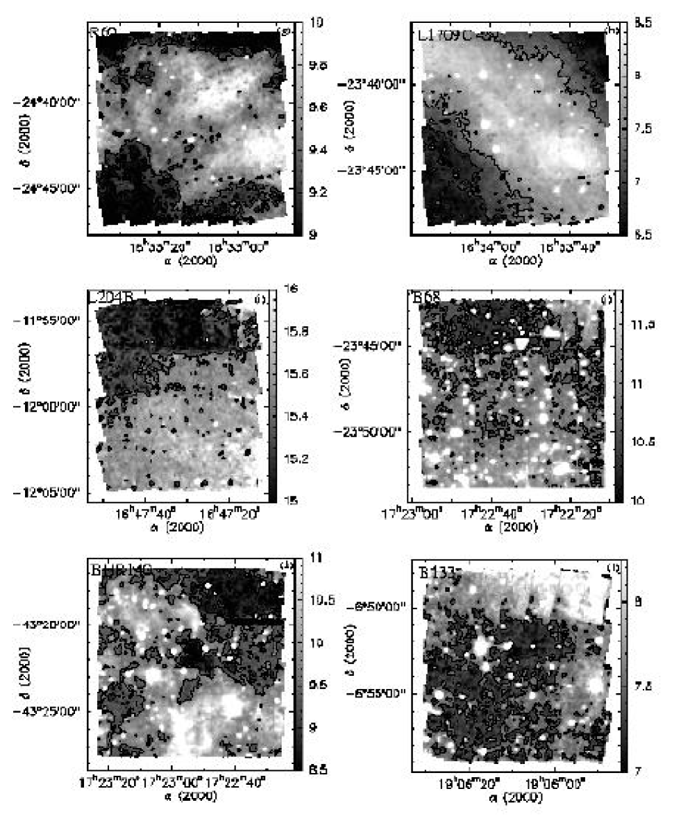
Figure 2: (cont’d) Contour levels: g) for R60, 9.1, 9.3 MJy/sr; h) for L1709C, 6.9, 7.4 MJy/sr; i) for L204B, 12.2 MJy/sr; j) for B68, 5.4, 5, 6 MJy/sr; k) for BHR140, 9, 9.5 MJy/sr; l) for B133, 7.4 MJy/sr.

3.1 ISOCAM images

Out of the 24 dark cloud fields in our programme, 23 show absorption-like features in the mid-IR.

Figure 3: (a) North-South intensity cut through the $\lambda=7.75$ $\mu$m ISOCAM image of L328 (see Fig. 1), at $\alpha\sim 18^{h}17^{m}00\aas@@fstack{s}$ (b) North-South intensity cut through the $\lambda=6.75$ $\mu$m ISOCAM image of L1689B at $\alpha\sim 16^{h}34^{m}50\aas@@fstack{s}$ Both cloud cores clearly show up in absorption against the diffuse mid-infrared background.

The fields presenting such features can be divided into two broad categories, those that show deep ($\;\buildrel>\over{\sim}\;$ 10% - cf. column 9 of Table 1), compact absorption features likely associated with dense cores, and those presenting weaker ($\;\buildrel<\over{\sim}\;$ 10%) and more diffuse absorption whose nature is also more uncertain. Figure 1 presents the ISOCAM images of 11 fields with strong absorption features, to which we added the widely studied core L1544 (e.g. Ward-Thompson et al. 1994, Tafalla et al. 1998, Williams et al. 1999, Ohashi et al. 1999), and from which we withdrew L1709C (the absorption features lying in the corners of the image, making the analysis difficult). The remaining fields are presented in Fig. 2. Figure 3 shows examples of cuts through two of the deep absorption features (for L328 and L1689B). The morphologies encountered in the fields with compact absorption vary from spherical cores like L328 to more elongated, filamentary structures (e.g. L1689B, GF5).

3.2 Comparison with the millimeter continuum maps

All of the cores observed at 1.3 mm (Table 2) present extended, weak dust continuum emission which we were able to map. For all cores, the peak of the mid-IR absorption does correspond with a peak in the millimeter emission. This is illustrated in Fig. 4 which shows the mid-IR ISOCAM absorption contours superimposed on the 1.3 mm continuum maps of the eight cores positively detected at 1.3 mm (the maps of Oph D and L1544 are also shown in MAN98 and WMA99, respectively).

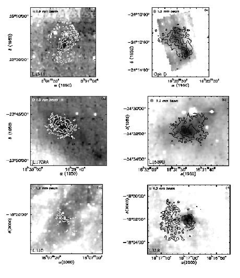
Figure 4: IRAM 1.3 mm continuum emission maps smoothed to 13$\arcsec$ FWHM resolution (contours) superimposed on ISOCAM 7 $\mu$m absorption image (greyscale). Contour levels are: a) 20, 40, 60 mJy/beam for L1544; b) 30, 50, 70 mJy/beam for Oph D; c) 20, 40, 60 mJy/beam for L1709A; d) 10, 30, 50 mJy/beam for L1689B; e) 20, 40, 60 mJy/beam for L310; f) 20, 40 mJy/beam for L328.

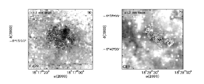
Figure 4: (cont’d) Contour levels are: g) 25, 50, 75, 100 mJy/beam for L429; h) 10, 20, 30, 40 mJy/beam for GF5.

The good agreement between the respective images of these cores in both types of data confirms that the features we see with ISOCAM are due to absorption by the (rather large) column density of cold dust traced at 1.3 mm, and not by fluctuations in the mid-IR background. Furthermore, the similar morphologies seen in both wavebands suggest that the mid-IR absorption images trace the same dust as the millimeter emission maps, which justifies a detailed comparison of the column density profiles derived from both tracers.

Table 2: Core parameters deduced from millimeter observations.

Name	$R_{flat}$	$N_{H_{2}}^{flat}$	$R_{out}$	$N_{H_{2}}^{out}$	$I_{zodi}^{MIR}$	$I_{fore}^{MIR}$	$I_{back}^{MIR}$
	(AU)	cm-2	(pc)	cm-2	(MJy/sr)	(MJy/sr)	(MJy/sr)
	(1)	(2)	(3)	(4)	(5)	(6)	(7)
L1544	1900	4.5 $\times 10^{22}$†	0.08	2$\times 10^{21}$	4.2	4.2${}^{+0.2}_{-0.7}$	0.7${}^{+0.7}_{-0.2}$
Oph D (LW2)	3400	5$\times 10^{22}$	0.05	3.2$\times 10^{21}$	5.7	5.7${}^{+1.5}_{-1.1}$	9.1${}^{+1.0}_{-1.3}$
Oph D (LW3)	“	“	“	“	45	42.1${}^{+2.6}_{-1.0}$	9.5${}^{+2.0}_{-2.4}$
L1709A	6400	4.5$\times 10^{22}$	0.18	3.1$\times 10^{21}$	10.5	11.3${}^{+0.6}_{-1.3}$	1.7${}^{+1.3}_{-0.6}$
L1689B s	4000	4$\times 10^{22}$	0.16	2$\times 10^{21}$	4.3	4.5${}^{+1.2}_{-1.0}$	3.8${}^{+1.0}_{-1.2}$
L1689B w	4000	4$\times 10^{22}$	0.29	4.8$\times 10^{21}$	4.3	4.3${}^{+1.0}_{-0.4}$	4.3${}^{+0.3}_{-0.7}$
L310	8000	1.7$\times 10^{22}$	0.11	1$\times 10^{21}$	7.1	7.1${}^{+0.3}_{-1.2}$	19.2${}^{+1.1}_{-0.2}$
L328	5000	3$\times 10^{22}$	0.14	2.4$\times 10^{21}$	7.4	7.4${}^{+6}_{-1.5}$	34.5${}^{+0.9}_{-5.3}$
L429	2400	5$\times 10^{22}$	0.26	8$\times 10^{21}$	6.8	6.8${}^{+0.2}_{-1.4}$	2.3${}^{+1.3}_{-0.1}$
GF5	5000	2$\times 10^{22}$	0.26	2$\times 10^{21}$	7.2	9.1${}^{+17.6}_{-2.5}$	70.8${}^{+1.5}_{-16.6}$

Notes to Table 2:

(1) $R_{flat}$ is the radius of the flat inner part of the core column density profile (see WMA99 and Sect. 3.4). For L1544, Oph D and L1689B, $R_{flat}$ was taken from the millimeter continuum measurements of WMA99 and corresponds to the geometrical average of the major and minor axes of the ellipse. For L1709A, L310, L328, L429 and GF5, $R_{flat}$ is the radius of the flat inner part of the ISOCAM profile.

(2) $N_{H_{2}}^{flat}$ is the column density averaged over the flat inner region of the core of radius $R_{flat}$ as deduced from our millimeter continuum measurements (see section 3.3.1).

(3) $R_{out}$ is the radius at which the C¹⁸O column density was measured in the outer parts of the core (see section 3.3.2).

(4) $N_{H_{2}}^{out}$ is the column density inferred from C¹⁸O(1-0) observations at $R_{out}$ (see section 3.3.2).

(5) $I^{MIR}_{zodi}$ is the zodiacal light emission in the mid-IR (see col. [8] of Table 1).

(6), (7) $I_{back}^{MIR}$ & $I_{fore}^{MIR}$ are the mid-IR background and foreground intensities as deduced from Eq. (1) and the values of the central and outer column densities, using the additional constraint that $I_{fore}\geq I_{zodi}$ (see section 3.3.3).

^†The values of $N_{H_{2}}^{flat}$ and $<N_{H_{2}}>_{13\arcsec}$ given in Table 2 of WMA99 are too large by $\sim$15 % and $\sim$ 70 %, respectively.

3.3 Modelling of the mid-infrared absorption

In order to derive information about the column density structure from the mid-IR intensity, we have used a simple geometrical model: each dense core is embedded within a lower-density parent molecular cloud. On the line of sight to the core, we measure i) a background intensity arising from the rear side of the parent cloud that is attenuated by the absorption from the core, and ii) a foreground intensity arising from the front side of the parent cloud. We can thus express the mid-IR intensity along the line of sight as:

$$I(\bar{r}) = [<I_{back}>+\delta I_{back}(\bar{r})]\cdot e^{-\tau_{\lambda}(\bar{r})}$$ (1)

$$+[<I_{fore}>+\delta I_{fore}(\bar{r})],$$

where $I_{back}$ and $I_{fore}$ are the background and foreground intensities respectively, and $\tau_{\lambda}(\bar{r})$ is the dust opacity at a projected radius $\bar{r}$ from core center and at observed wavelength $\lambda$. The foreground emission, $I_{fore}(\bar{r})$, includes the contribution from the zodiacal light emission, $I_{zodi}$.

The mid-infrared background emission, $I_{back}(\bar{r})$, is thought to arise from very small grains presenting aromatic emission features (Léger & Puget 1984, Allamandola, Tielens & Barker 1989, Boulanger et al. 1996). These grains/molecules are excited by the interstellar far-UV (FUV) radiation field and re-emit this energy as a group of spectral lines/bands in the mid-infrared, the Unidentified Infrared Bands (UIBs). The ISOCAM LW2=[5.0, 8.5 $\mu$m] and LW6=[7.0, 8.5 $\mu$m] filters that we used for our observations include the 6.2 $\mu$m and 7.7 $\mu$m emission features of these UIBs.

According to recent studies, the small particles responsible for the UIBs are distributed throughout molecular clouds but because of high interstellar extinction in the FUV band, they are ususally only excited in the outer regions where $A_{v}\lower 2.15277pt\hbox{$\;\buildrel<\over{\sim}\;$}1$ (Hollenbach & Tielens 1997, Bernard et al. 1993). For this reason, the interiors of (quiescent) clouds should be relatively free of UIB emission, and only their outer envelopes should significantly contribute to the mid-IR background and foreground (e.g. Bernard et al. 1993, Boulanger et al. 1998).

As a first step, we neglected the spatial fluctuations of the background and foreground, $\delta I_{back}(\bar{r})$ and $\delta I_{fore}(\bar{r})$, and thus assumed $I_{back}$ and $I_{fore}$ to be equal to their mean values across the field, $<I_{back}>$ and $<I_{fore}>$ (see 3.5.2 below for a critical discussion of this assumption).

For a given gas-to-dust ratio, the H₂ column density $N_{H_{2}}$ is related to the dust opacity by $\tau_{\lambda}(\bar{r})=\sigma_{\lambda}\cdot N_{H_{2}}(\bar{r})$, where $\sigma_{\lambda}$ is the dust extinction cross section at the wavelength of observation $\lambda$. We assume $\sigma_{\lambda}$ to follow the Draine & Lee (1984) dust model in the mid-IR as a first approximation, but the value is rather uncertain (see section 3.5). We adopted $\sigma_{6.75\mu m}=1.2\times 10^{-23}$ cm² for the LW2 filter, $\sigma_{7.75\mu m}=1.35\times 10^{-23}$ cm² for the LW6 filter, and $\sigma_{15\mu m}=1.6\times 10^{-23}$ cm² for the LW9 filter, i.e., we calculated $\sigma_{\lambda}$ at the central wavelength of each filter. A more accurate value could be obtained by integrating the extinction curve over the response of the ISOCAM filters, but as we will see in the following, the exact value of $\sigma_{\lambda}$ has only little influence on the derived column density profiles.

The quantities $I_{back}$ and $I_{fore}$ are unknown, but they can be constrained using independent measurements of the H₂ column density at two different radii. These constraints enable the ISOCAM absorption profile to be converted into a column density profile.

3.3.1 Central column density from millimeter continuum data

We used our 1.3 mm continuum maps to estimate the column density averaged over the flat central region of each core. As millimeter dust continuum emission is optically thin, the column density averaged over the flat inner part (of radius $R_{flat}$) of the core (see WMA99) may be derived from the 1.3 mm flux density integrated over the same area, $S_{1.3mm}^{flat}$ (cf. AWM96, MAN98):

$$N^{flat}_{1.3mm}=S^{flat}_{1.3mm}/[\Omega^{flat}\kappa_{1.3mm}\mu m_{H}B_{1.3mm}(T)],$$ (2)

where $\Omega^{flat}$ is the solid angle of the flat inner region, $\kappa_{1.3mm}$ is the dust opacity per unit mass column density at $\lambda$ = 1.3 mm, $\mu=2.33$ is the mean molecular weight, and $B_{1.3}(T)$ is the Planck function at $\lambda$ = 1.3 mm, for a dust temperature $T$. We assumed a single, representative dust temperature $T_{d}=12.5$ K for all the cores. Based on recent ISOPHOT measurements of L1544, Oph-D, L1689B, and other similar starless cores (e.g. Ward-Thompson & André 1999, Lehtinen et al. 1998), we believe that this value of $T_{d}$ is likely to be within $\pm 3$ K of the true dust temperature in most cases. Considering the additional uncertainty on the millimeter dust mass opacity in dense cores, which we took equal to $\kappa_{1.3mm}=0.005$ cm²g^-1 (see, e.g., Preibisch et al. 1993, AWM96, and Kramer et al. 1999), the estimates of $N_{H_{2}}^{flat}$ listed in Table 2 are uncertain by a factor of $\lower 2.15277pt\hbox{$\;\buildrel>\over{\sim}\;$}2$ on either side of their nominal values.

3.3.2 Outer column density from millimeter line data

The second value of the column density we can use to calibrate the ISOCAM column density profile is given by our C¹⁸O(1-0) line observations of the outer parts of the cores. Assuming optically thin emission and Local Thermodynamical Equilibrium (LTE), we can determine the value of the C¹⁸O column density from the following equation:

$$N_{C^{18}O}(cm^{-2})=4.76\times 10^{13}\frac{T_{k}+0.88}{\exp(-\frac{5.27}{T_{k}})}\int_{-\infty}^{+\infty}T_{A}^{*}(v)dv,$$ (3)

where $T_{A}^{*}$ is the measured antenna temperature of the C¹⁸O(1-0) line, $T_{k}$ is the gas kinetic temperature in the cloud, and $dv$ is in km s^-1 (e.g. Rohlfs & Wilson 1996). We used Eq. (2) with $T_{k}=10$ K to estimate the C¹⁸O column density in the outer parts of the core. This method would not be reliable towards the center of the core where C¹⁸O(1-0) may be optically thick. Moreover at the centre, the possibility of depletion of gas molecules onto grains makes the estimation of the column density unreliable (e.g. Kramer et al. 1999). We adopted the following relation between H₂ and C¹⁸O column densities (Frerking, Langer & Wilson 1982): $N_{H_{2}}=5.53\times 10^{6}N_{C^{18}O}+1.22\times 10^{21}$ cm^-2. The values of the column density $N_{H_{2}}^{out}$ derived in this way, as well as the distance $R_{out}$ from the core centre at which it was evaluated, are given in Table 2. The exact position where $N_{H_{2}}^{out}$ was measured is indicated by a triangle-symbol on the images of Fig. 1. The uncertainty on the H₂ column density derived from molecular line data has two major origins: first, the excitation state of the C¹⁸O(1-0) molecules is not accurately known and the LTE hypothesis is only an approximation (cf. White et al. 1995), and second, the C¹⁸O abundance ratio with respect to H₂ is also uncertain in our cores. Based on comparisons with more sophisticated calculations performed with a Monte-Carlo radiative transfer code (Blinder 1997) for a realistic pre-stellar core model, we judge that our LTE estimate of the column density in the outer parts of each core, $N_{H_{2}}^{out}$, is good to better than a factor of $\sim 2$.

3.3.3 Estimates of the background and foreground intensities

Given the values of $N_{H_{2}}^{flat}$ and $N_{H_{2}}^{out}$ derived from millimeter observations, it is easy to estimate $I_{back}$ and $I_{fore}$ using Eq (1) for $\bar{r}=R_{flat}$ and $\bar{r}=R_{out}$, and then deduce the column density from the mid-IR intensity at any position in the ISOCAM image. The values of $I_{back}$ and $I_{fore}$ that we calculated in this way, using the independent constraints that $I_{back}\geq 0$ and $I_{fore}\geq I_{zodi}$, are listed in Table 2. In addition to ‘best’ values, we give permitted ranges for $I_{back}$ and $I_{fore}$ that were determined using the maximum and minimum values of $N_{H_{2}}^{out}$ and $N_{H_{2}}^{flat}$ (given the factor $\sim 2$ uncertainty on both these quantities).

Another approach consists in estimating the values of $I_{back}$ and $I_{fore}$ directly from the ISOCAM images. The sum $I_{back}+I_{fore}$ is constrained by the mean mid-IR intensity $<I_{MIR}>$ measured in the map outside the dense core (cf. column 7 of Table 1; this also corresponds to the “baseline level” measured on intensity cuts such as those of Fig. 3). Furthermore, one can set straightforward lower and upper limits on the foreground intensity since $I_{fore}$ has to be less than the value of the minimum intensity in the image, $I_{min}$, and greater than the zodiacal emission, $I_{zodi}$. Hence, $I_{zodi}<I_{fore}<I_{min}$ and, since $I_{back}+I_{fore}=$  $<I_{MIR}>$,   $<I_{MIR}>-I_{min}$  $<I_{back}<$ $<I_{MIR}>-I_{zodi}$.

This second method assumes that $<I_{MIR}>$ can be measured outside the dense core, which is not necessarily the case if, e.g., the core extends beyond the limits of the ISOCAM map. Moreover, according to Eq. (1), the minimum intensity in the image is equal to the intensity at the maximum of the absorption ($I_{min}=<I_{back}>\cdot e^{-\tau_{max}}+<I_{fore}>$), which in practice can greatly overestimate the value of $<I_{fore}>$ since one typically has $\tau_{max}\lower 2.15277pt\hbox{$\;\buildrel<\over{\sim}\;$}1$ (see below). For these reasons, we preferred to adopt the first approach based on millimeter measurements of the central and outer column densities (see above).

In the case of the Oph D dense core, however, it is possible to determine accurate values of $I_{back}$ and $I_{fore}$ at more than one wavelength using both methods, since large-scale ($\sim 0.8\degr\times 0.8\degr$) ISOCAM images of the $\rho$ Oph main cloud are available (cf. Abergel et al. 1996). This provides an important consistency check. At 6.75 $\mu$m, we obtain $I_{fore}^{6.75}=5.7^{+1.5}_{-1.1}$ MJy/sr and $I_{back}^{6.75}=9.1^{+1.0}_{-1.3}$ MJy/sr using millimeter observations (see Table 2), while we find $4.6$ MJy/sr $<I_{fore}^{6.75}<8.5$ MJy/sr and $6.3$ MJy/sr $<I_{back}^{6.75}<10.2$ MJy/sr using the second method. The agreement is thus very good. The background and foreground intensities can also be estimated at $\sim 15$ $\mu$m (cf. Table 2). As can be seen in Fig. 5c) and 5d) below, they yield a column density profile for Oph D which is virtually identical to that derived at 6.75 $\mu$m. Furthermore, our estimated values ($I_{fore}^{15}=42.1^{+2.6}_{-1.0}$ MJy/sr and $I_{back}^{15}=9.5^{+2.0}_{-2.4}$ MJy/sr) are consistent with the idea that the mid-IR background is primarily due to the emission of UIB carriers while the foreground is dominated by the zodiacal light. Indeed, the emission spectrum of aromatic particles is such that the ratio of the LW2-filter to LW3-filter intensities is $\sim 1$ (Boulanger et al. 1996), which is precisely what we find for the background emission in Oph D. By contrast, the 7–15 $\mu$m spectrum of the foreground emission is rising and compatible with that of the zodiacal light ($I_{zodi}\sim 5.7$ MJy/sr at $\sim 7$ $\mu$m and $I_{zodi}\sim 45$ MJy/sr at $\sim 15$ $\mu$m).

The results of these inter-comparisons on Oph D confirm the validity of the millimeter method we used to determine $I_{back}$ and $I_{fore}$ for the other cores.

We note that for many sources $I_{fore}\sim I_{zodi}$ in Table 2, suggesting that the zodiacal emission is often the main contributor to the foreground. This situation is expected if most of the target clouds are illuminated from behind, which is indeed believed to be the case for the $\rho$ Oph cloud, located in front of the Sco OB2 association (e.g. de Geus et al. 1989, de Geus 1992). As most of our fields were chosen to be nearby and devoid of strong (e.g. foreground) infrared sources, the fact that the front sides of the clouds appear to contribute negligible foreground emission is likely the result of a selection effect.

3.4 Radial column density profiles

3.4.1 Derivation of the profiles

In order to characterize the radial structure of each core and reduce the influence of spatial fluctuations in the background and foreground, we first derived mean radial intensity profiles by averaging the mid-IR emission in the ISOCAM images according to the apparent morphology of the core. For L1689B, we averaged the intensity over elliptical annuli of increasing radii separately for a 40°sector in the South and a 40°sector in the Western side of the core. For L328, OphD and L429, the intensity was averaged over circular annuli of increasing radius. Only the South-Western sector of the profile was considered for Oph D and only the Western half for L328. For very elongated, filamentary structures (L310, L1709A, L1544, GF5), we averaged cuts perpendicular to the main axis of the cores, but only kept the Southern half of the absorption intensity profile (except GF5 for which the North side was kept). The sectors over which the profiles were averaged (for the elliptically/spherically symmetric cores L1689B, L328 and L429) are shown as dotted lines on Fig. 1 as are the ranges of cuts which were averaged for the filamentary cores (L1544, L1709A, L310, GF5).

The radial column density profiles $N_{H_{2}}^{0}(\bar{r})$ that were derived in this way using our ‘best’ values for $I_{back}$ and $I_{fore}$ (see above) are displayed in Fig. 5 as crosses. The vertical cross sizes represent statistical error bars on the mean radial profile, estimated from the dispersion of the values averaged at each radius, divided by the square root of the number of values. In addition to these random errors at each radius, there is also a global uncertainty on the column density profiles resulting from our uncertain knowledge of $I_{back}$ and $I_{fore}$. The dashed curves lying above and below the ‘best’ profiles limit the range of column density profiles that are consistent with the mid-IR absorption data, given the permitted range of values for $I_{back}$ and $I_{fore}$ in each case (see Table 2). The upper dashed curve corresponds to the profile for the smallest value of $I_{back}$ and the greatest value of $I_{fore}$, while the lower dashed curve corresponds to the greatest value of $I_{back}$ and the smallest value of $I_{fore}$. It is important to stress that there is a simple, global relation between each permitted profile, $N_{H_{2}}(\bar{r})$, and the ‘best’ profile, $N_{H_{2}}^{0}(\bar{r})$, of the type:

$$N_{H_{2}}(\bar{r})=\frac{1}{\sigma_{\lambda}}\cdot\ln\biggl{(}\frac{1}{A\,e^{-\sigma_{\lambda}N_{H_{2}}^{0}(\bar{r})}+B}\biggr{)},$$

where $A$ and $B$ are two parameters depending only on $N_{H_{2}}^{flat}$ and $N_{H_{2}}^{out}$, and $\sigma_{\lambda}$ is again the extinction cross-section at the mid-IR wavelength $\lambda$.

For comparison with the profiles derived from the ISOCAM images, the thin solid curves in Fig. 5 represent the column density profiles of finite-sized sphere models with uniform density for $r<R_{flat}$, $\rho\propto r^{-2}$ for $R_{flat}<r<R_{edge}$, and surrounded by a medium of uniform column density. The dotted curves plotted in Fig. 5 are $N_{H_{2}}\propto\bar{r}^{-1}$ power laws (which correspond to the column density profile of a singular isothermal sphere at 10 K). These models as well as other theoretical models will be discussed in Sect. 4. (Note that the convolution with the ISOCAM psf has no effect on the models beyond an angular radius of $\sim$ 6$\arcsec$.)

Table 3: Core parameters derived from the ISOCAM absorption analysis

Source	$N_{H_{2}}^{flat}$	$N_{H_{2}}^{peak}$	$\tau_{max}^{7\mu m}$	$R_{flat}^{ISO}$	$R_{mid}^{ISO}$	$R_{edge}^{ISO}$	$n_{H_{2}}^{flat}$	$M_{flat}$	$M_{edge}$	$m_{1}$	$m_{2}$	$\frac{n_{flat}}{n_{out}}$
Name	(cm-2)	(cm-2)		(0.01 pc)	(pc)	(pc)	(cm-3)	(M⊙)	(M⊙)
	(1)	(2)	(3)	(4)	(5)	(6)	(7)	(8)	(9)	(10)	(11)	(12)
L1544	5.4$\times$1022	6.0$\times$1022	0.7	1.4	0.028	0.043	4$\times$105	0.5	1.9	$-$1.6${}^{+0.1}_{-0.2}$	$-$4.4${}^{+0.7}_{-0.1}$	20
Oph D	5$\times$1022	6.6$\times$1022	0.7	1.6	0.028	0.066	3.0$\times$105	0.8	2.0	$-$0.8${}^{+0.1}_{-0.2}$	$-$2.8${}^{+0.7}_{-2.6}$	80
L1709A	4.5$\times$1022	5.1$\times$1022	0.6	3.2	0.18	$>$0.32	1.2$\times$105	2.4	$>$29	$-$1.2${}^{+0.5}_{-0.4}$	-	70
L1689B	4.5$\times$1022	5.8$\times$1022	0.7	3.2	0.096	0.136	1.4$\times$105	2.2	11	$-$1.4${}^{+0.3}_{-0.2}$	$-$4.3${}^{+1.9}_{-2.9}$	50
(South)
L1689B	4.7$\times$1022	6.0$\times$1022	0.7	4	0.28	$>$0.40	1.2$\times$105	3.5	$>$70	$-1.0^{+0.4}_{-0.8}$	-	50
(West)
L310	3.4$\times$1022	3.7$\times$1022	0.5	4	0.07	0.1	9$\times$104	1.5	7.7	$-$1.5${}^{+0.1}_{-0.1}$	-	$>$10
L328	4.4$\times$1022	5.8$\times$1022	0.8	2.5	0.03	0.12	1.8$\times$105	1.1	6.4	$-$1.7${}^{+0.4}_{-0.7}$	$-$1.7${}^{+0.4}_{-0.7}$	$>$20
L429	9.6$\times$1022	1.2$\times$1023	1.6	$\sim$1.2	0.35	$>$0.5	6$\times$105	$\sim$0.4	$>$60	$-$0.9${}^{+0.5}_{-0.5}$	-	$>$600
GF5	2.7$\times$1022	3$\times$1022	0.4	2.5	0.2	$>$0.4	1$\times$105	0.7	$>$30	$-$0.9${}^{+0.2}_{-0.2}$	-	$>$140

Notes to Table 3:

(1) Column density averaged over the flat inner part of the core of radius $R_{flat}^{ISO}$.

(2) Peak column density read from the ISOCAM profiles of Fig. 5.

(3) Opacity at the centre of the core at $\sim$ 7 $\mu$m.

(4) $R_{flat}^{ISO}$ is the radius of the flat inner part of the ISOCAM profiles of Fig. 5 and is slightly different from $R_{flat}$ (cf. Table 2) for L1544, Oph D and L1689B.

(6) Radius of the core edge (when there is one).

(7) Average density over the flat inner core region, estimated from a piecewise power-law model fitting the profile (see text).

(8) Integrated core mass within a circular area of radius $R_{flat}^{ISO}$.

(9) Integrated core mass within a circular area of radius $R_{edge}^{ISO}$.

(10) Index of the power-law fitting the column density profile between $R_{flat}^{ISO}$ and $R_{mid}^{ISO}$ (Column 4).

(11) Index of the power-law fitting the column density profile between $R_{mid}^{ISO}$ (Column 4) and $R_{edge}^{ISO}$.

(12) Density contrast between the centre and the edge of the core. For Oph D, L1689B and L1709A, the value of $n_{out}$ was taken from the large scale ¹³CO observations of Loren (1989a), and for L1544, it comes from Butner et al. (1995). As no estimate of $n_{out}$ is available for the remaining cores in the literature, a lower limit for the density contrast was estimated from the model described in Section 4.1.

3.4.2 Results

It can be seen from Fig. 5 that all the column density profiles present a flattening in their inner regions - though this flattening is only marginal in the case of L429. On the other hand, the slopes and shapes of the outer parts of the profiles appear to vary from core to core and may be separated into two broad categories. For four of the cores (GF5, L429, L1709A and the Western part of L1689B), the profile beyond the flat inner part follows a near power law with projected radius $\bar{r}$, i.e. $N_{H_{2}}\propto\bar{r}^{-1}$, and does not show any clear steepening up to the boundary of the image. By contrast, for the other cores (L328, Oph D, L310, L1544 and the Southern side of L1689B), the profile steepens beyond some radius $R_{mid}$, until it merges with the ambient molecular cloud. Three cores in our sample present “edges”, defined as regions where the column density profile drops significantly steeper than a $N_{H_{2}}\propto\bar{r}^{-1}$ power law. Globally, we may divide each column density profile into four parts: a flat inner region of radius $R_{flat}^{ISO}$, followed by a near power-law portion of index $m_{1}$ up to a radius $R_{mid}^{ISO}$, a region with a steep slope $m_{2}$ from $R_{mid}^{ISO}$ to $R_{edge}^{ISO}$ that marks the core “edge”, and finally a relatively flat plateau once the column density has reached the average value it has in the ambient molecular cloud. Depending on the cases, one or two parts may be absent.

The values of the core opacities at 7 $\mu$m, the column densities, as well as the masses, average slopes, and density contrast deduced from the ISOCAM profiles of Fig. 5 are given in Table 3. The peak column density, $N^{peak}_{H_{2}}$, was read on the profiles shown in Fig. 5. (In most cases, $N^{peak}_{H_{2}}>N^{flat}_{H_{2}}$ because the central plateau is not strictly flat). The average slopes $m_{1}$ and $m_{2}$ of the column density profile between $R_{flat}^{ISO}$ and $R_{mid}^{ISO}$, and between $R_{mid}^{ISO}$ and $R_{edge}^{ISO}$, respectively, were derived by fitting segments of straight lines to the data. The maximum values of $m_{1}$ and $m_{2}$ were obtained by assuming the maximum possible value of $N^{flat}_{H_{2}}$ together with the minimum possible value of $N_{H_{2}}^{out}$ (taking into account the factor of $\sim$ 2 uncertainty), while the minimum values of $m_{1}$ and $m_{2}$ were obtained by assuming the minimum possible value of $N^{flat}_{H_{2}}$ together with the maximum possible value of $N_{H_{2}}^{out}$.

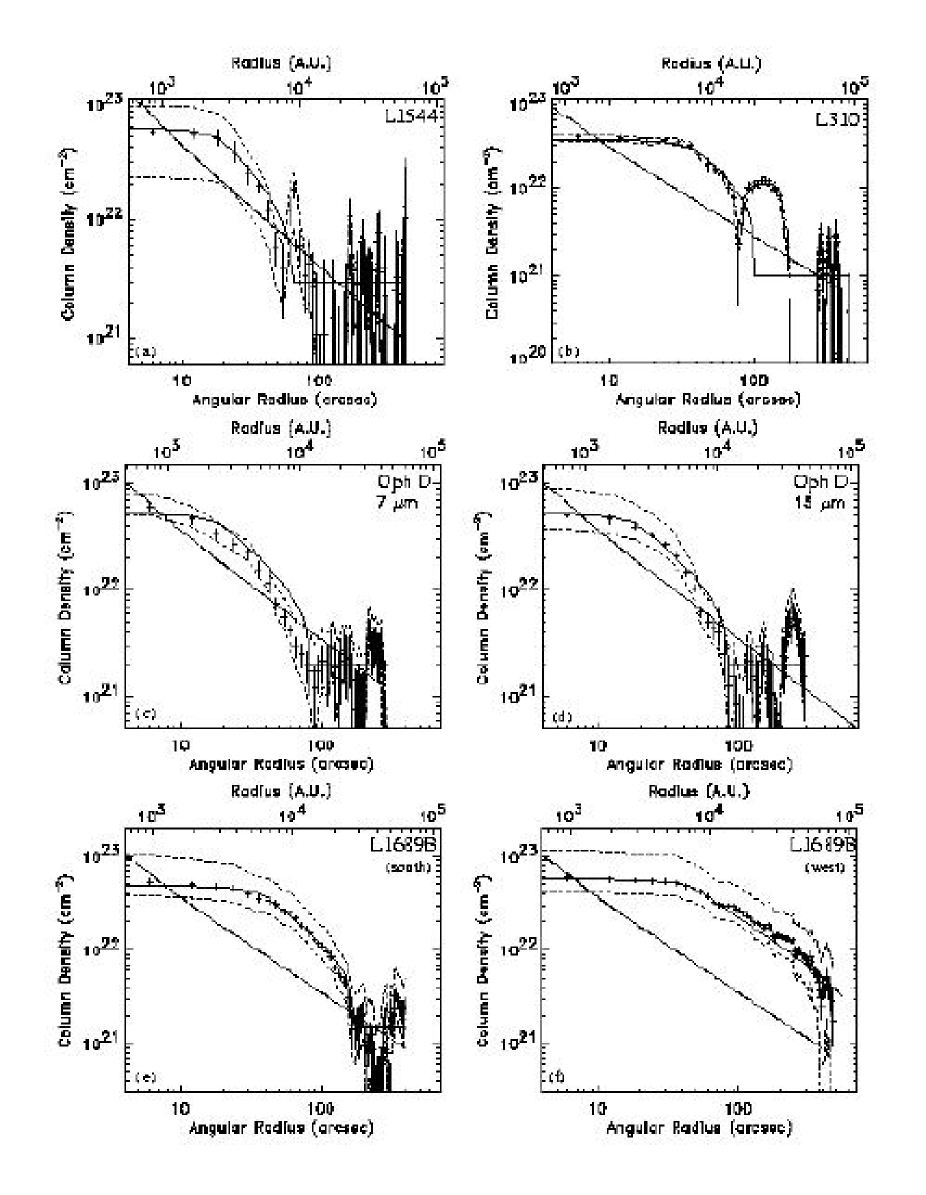
Figure 5: Column density profiles of the target pre-stellar cores (crosses), as well as global error bars (dashed curves), derived from the ISOCAM images and adjusted so as to match the values obtained in the flat central region with 1.3 mm continuum data and in the outer region with C¹⁸O(1–0) line observations (see § 3.3). Theoretical models are plotted for comparison (see § 4).

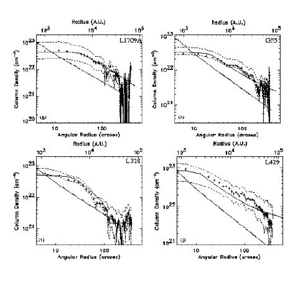
Figure 5: (cont’d) The dotted line is an $N_{H_{2}}\propto\bar{r}^{-1}$ power-law (corresponding to the profile of a singular isothermal sphere at T=10 K), convolved with the ISOCAM psf. The thin solid line corresponds to the column density profile of a finite-sized sphere model with uniform density for $r<R_{flat}$, $\rho\propto r^{-2}$ for $R_{flat}<r<R_{edge}$, and surrounded by a medium of uniform column density.

3.5 Uncertainties, difficulties, limitations

3.5.1 Dust extinction curve in the mid-IR

Among the parameters involved in the relationship between the mid-IR intensity and the H₂ column density is the dust extinction coefficient $\sigma_{\lambda}$. This paragraph focuses on the influence of $\sigma_{\lambda}$ on the derived column density profiles. The uncertainty on $\sigma_{\lambda}$ stems from two main factors. First, the ISOCAM filters encompass a certain bandwidth over which the value of $\sigma_{\lambda}$ varies. In our study, we used for $\sigma_{\lambda}$ the value for the wavelength at the centre of the filter (ie at 6.75 $\mu$m for the LW2 filter and 7.75 $\mu$m for the LW6 filter). Considering the rapid variations (steep increase) of $\sigma_{\lambda}$ towards 8 $\mu$m (eg. Draine & Lee 1984), the values we adopted in § 3.3 above could be underestimated by up to a factor of $\sim$ 2. Second, the dust properties in dense cores are known to depart from those calculated by Draine & Lee (1984) for the diffuse interstellar medium (Krügel & Siebenmorgen 1994, see in particular their Fig. 12). In environments like dense cores, in which temperatures can be as low as $\sim$10 K and densities as high as $\sim 10^{5}$-$10^{6}$ cm^-3, coagulation of particles, fluffiness and the presence of ice mantles on the grains can change the value of the dust extinction coefficient, depending on the nature of the grains (amorphous carbon or coated silicate grains). By using the Draine & Lee value, we could thus be underestimating the value of the extinction coefficient by a factor of $\sim$ 2.

To check how the column density profile was affected by the value of $\sigma_{\lambda}$, we calculated it for different values of $\sigma_{\lambda}$. As the innermost parts of the core are denser and more shielded from the interstellar radiation field (and thus colder), they are more likely to be affected by grain coagulation and forming of ice mantles, resulting in a higher extinction coefficient than in the low-density outer parts. We therefore determined the column density profiles supposing a linear increase of $\sigma_{\lambda}$ from 1.35$\times 10^{-23}$cm² on the edges of the core to 2.7$\times 10^{-23}$cm² (which is twice the previous value) at the centre of the core. We also varied the value of $\sigma_{\lambda}$ by factors of 2 and 3 to check the influence of a high value of $\sigma_{\lambda}$ on the shapes of the profiles.

The results of this study show that if $\sigma_{\lambda}$ varies within a factor of $\sim$ 2–3 the column density profiles change only marginally. The same holds true if we assume a linear gradient in $\sigma_{\lambda}$ or in Log($\sigma_{\lambda}$) from the centre to the edge of the cloud (so that in the end $\sigma_{\lambda}$ varies within a factor of 2). To summarize, our conclusions regarding the slopes of the column density profiles are not sensitive to the existing uncertainties on $\sigma_{\lambda}$.

3.5.2 Simulations of non uniform background and foreground intensities

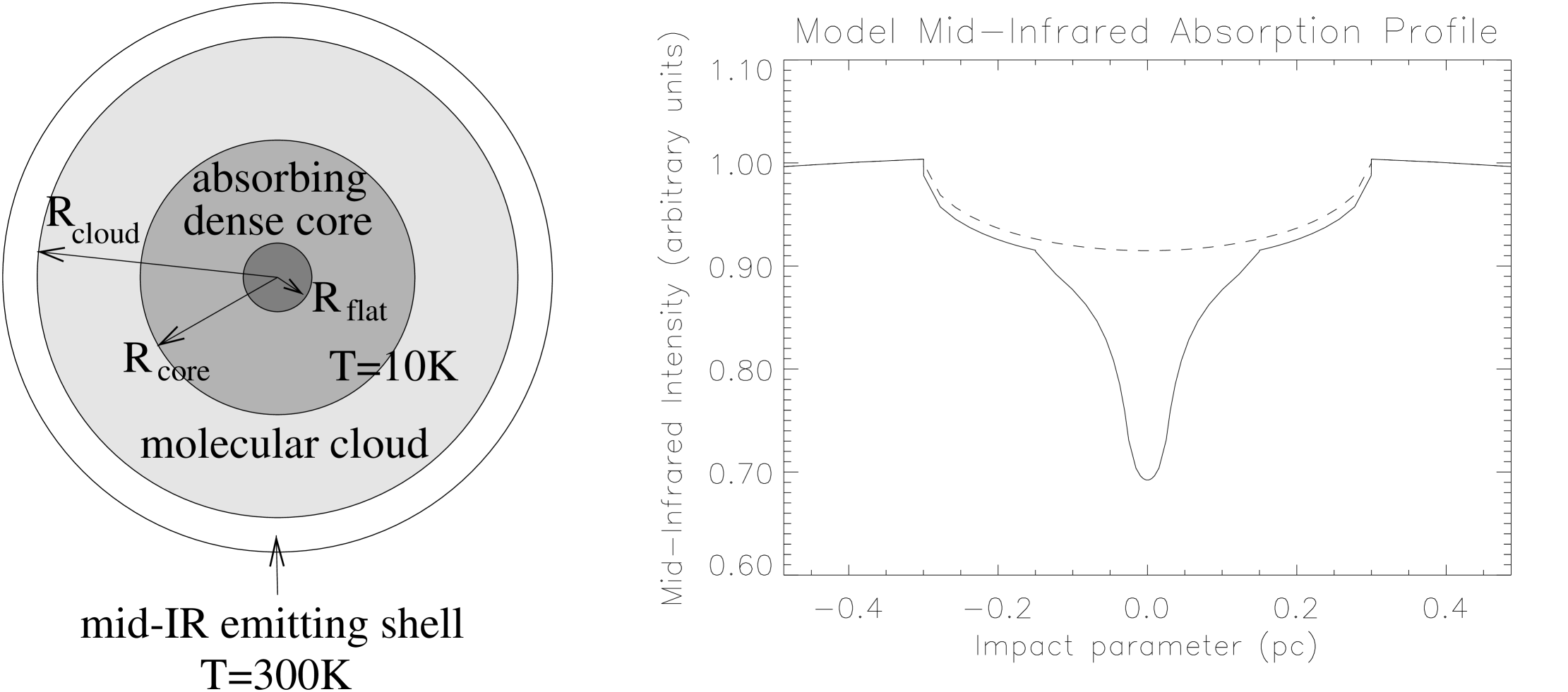
Figure 6: Schematic representation of the simple model cloud/core system discussed in the text (left panel). The right panel shows the simulated mid-IR intensity profile (solid curve) emerging from such a model. The dashed curve represents what the intensity profile would be without the absorbing dense core/cloud. The illustrative case shown has $R_{flat}=0.025$ pc, $R_{core}=0.15$ pc, and $R_{cloud}=0.3$ pc. Note some similarity with the observed profiles of Fig. 3.

To check the influence of our assumption that the foreground and background intensities are spatially uniform, we carried out simulations of the total infrared intensity measured by the camera (and of the column density inferred), if the absorbing dense core is embedded in an ambient cloud of uniform column density, itself bounded by a mid-IR emitting shell (cf. Fig. 6 – left panel). We considered a spherically symmetric core model with uniform density for $r<R_{flat}$, $\rho\propto r^{-2}$ for $R_{flat}<r<R_{core}$ (corresponding to a $N\propto\bar{r}^{-1}$ column density profile), and uniform temperature $T_{in}\sim 10$ K throughout. (This is similar to the simple model compared to the data in Fig. 5 and discussed in Sect. 4.1 below.) The parent cloud (corresponding to radii $R_{core}<r<R_{cloud}$) is also assumed to be at $T_{in}\sim 10$ K. By contrast, the outer shell (beyond $R_{cloud}$) is taken to be much warmer at $T_{out}\sim 300$ K, so that its maximum emission is in the mid-IR. Thus, we have a thin outer region emitting mid-IR radiation and a cold, dense inner cloud/core only absorbing in the mid-IR. Such an idealized model of emission by an outer cloud in thermal equilibrium at $T_{out}\sim 300$ K is clearly not realistic and only meant to be illustrative of a background medium emitting in the mid-IR. Since it is the thin spherical shell beyond $R_{cloud}$ that produces the background and foreground, $I_{back}$ and $I_{fore}$ are not uniform in this model but present ‘limb-brightened’ peaks at $\bar{r}=R_{cloud}$ (see Fig. 6 – right panel).

When $R_{core}$ is significantly smaller than $R_{cloud}$, our simulations show that $I_{back}$ and $I_{fore}$ vary only slowly over the spatial extent of the absorbing dense core (see the example of Fig. 6). In such a situation, the column density profile derived from the simulated mid-IR intensity of the model in the same way as for the ISOCAM data is almost indistinguishable from the original model profile. On the other hand, if $R_{core}\sim R_{cloud}$ so that the peaks in $I_{back}$ and $I_{fore}$ occur immediately outside the core, then the profile derived under the assumption that $I_{back}$ and $I_{fore}$ are spatially uniform departs markedly from the true column density profile as the temperature discontinuity is approached for $\bar{r}\sim R_{cloud}$. In particular, the derived profile drops sharply near $R_{core}$, i.e., displays a sharp edge, even when the warm outer shell has the same $\rho\propto r^{-2}$ density profile as the cold inner cloud core (so that there is no physical edge in the density structure but only a discontinuity in temperature). This shows that our method of converting intensities into column densities enables us to detect the existence of a discontinuity, but does not necessarily allow us to conclude about its nature.

Table 4: Values of reduced $\chi^{2}$ for the various theoretical models

Source	Parameterized	Logotrope	best fitting SIS1	BM95	CM95
	Sphere
L1544	5.9	8.2	25.8	11.3	5.2
Oph D	1.3	13.4	23.0	19.9	1.3
L1709A	3.0	5.5	8.8	3.0	-
L1689B s	1.0	9.8	29.4	1.2	17.7
L1689B w	3.2	47.2	241.7	3.7	21.1
L328	4.3	30.8	19.5	49.7	6.8
L429	19.2	15.4	14.3	5.7	-
GF5	8.0	4.4	54.0	3.3	-

Notes:

The $\chi^{2}$ calculations were restricted to radii smaller than $R_{edge}$ (Table 3) for cores with an edge.

¹ The SIS model considered in this Table is the one that fits best the near power-law portion of the column density profile. It corresponds to gas temperatures higher than 10 K.

In practice, however, it seems reasonable to assume that we are in the situation of Fig. 6 and that $I_{back}$ and $I_{fore}$ have nearly uniform values over distance scales of several tenths of parsecs. The $\rho$ Ophiuchi cloud complex may be used as an example. In this case, there is convincing evidence from the IRAS study of Bernard et al. (1993) that the mid-IR background emission originates from photo-excited PAH-like molecules distributed in a sort of shell corresponding to the outer layers of the large-scale ¹³CO molecular cloud mapped by Loren (1989). This geometry is very reminiscent of Fig. 6 with $R_{cloud}$ on the order of a few pc, i.e., much bigger than the rather small ($R_{core}\sim 0.1$ pc) cores we are studying here (see, e.g., Table 3). This means that the cores are embedded deep inside the layers responsible for the mid-IR emission. Another piece of evidence comes from the ISOCAM images themselves which do not show strong intensity fluctuations on small scales.

4 Discussion: Comparison with theoretical models of core structure

As pointed out in Sect. 3.4, the radial column density profiles derived for the pre-stellar cores of our ISOCAM absorption sample (see Fig. 5) are generally characterized by four different regimes: a) a flat inner region where the column density gradient is much flatter than $N_{H_{2}}\propto\bar{r}^{-1}$, b) a region roughly consistent with $N_{H_{2}}\propto\bar{r}^{-1}$, c) an edge where the column density gradient steepens quickly with distance from core center and gets as steep as $N_{H_{2}}\propto\bar{r}^{-2}$ or even steeper (see Table 3), until d) the end of the dense core is reached and $N_{H_{2}}$ fluctuates about the mean value in the parent cloud (i.e., typically $N_{out}\sim 2\times 10^{21}$ cm^-2).

In the simple case of an infinite spheroidal core with a power-law density structure, the radial density gradient, $\rho\propto r^{-p}$, is related to the column density gradient, $N_{H_{2}}\propto\bar{r}^{-m},$ by $p=m+1$ (e.g. Adams 1991, Yun & Clemens 1991). If alternatively, the core radial density structure is not represented by a single power law but by piecewise power laws, then the preceding relation between $p$ and $m$ is no longer strictly exact in the transition regions due to convergence effects. However, these effects can be quantified in specific cases. For instance, in the case of a sphere of uniform density at both small ($r<r_{0}$) and large ($r>r_{1}$) radii, and having $\rho\propto r^{-2}$ between $r_{0}$ and $r_{1}$, the column density profile gets somewhat steeper than $N_{H_{2}}\propto\bar{r}^{-1}$ between $r_{0}$ and $r_{1}$, but remains always shallower than $N_{H_{2}}\propto\bar{r}^{-1.4}$. For a similar sphere with $\rho\propto r^{-3}$ instead of $\rho\propto r^{-2}$ between $r_{0}$ and $r_{1}$, the column density profile is always shallower than $N_{H_{2}}\propto\bar{r}^{-2.2}$. We conclude that, if the column density profile is observed to become steeper than $N_{H_{2}}\propto\bar{r}^{-2.2}$, then we may safely infer that the underlying density profile becomes steeper than $\rho\propto r^{-3}$ at some neighboring radius. Note that this conclusion remains essentially valid even in the extreme case of a finite-sized sphere where the density drops to $0$ beyond a radius $R_{out}$ (cf. Arquilla & Goldsmith 1985, Yun & Clemens 1991). In such a case, both the density and the column density gradient become effectively infinite at $R_{out}$. Although the simple relation $p=m+1$ would yield too large values of $p$ in a narrow range of radii $r\lower 2.15277pt\hbox{$\;\buildrel<\over{\sim}\;$}R_{out}$, the basic conclusion that $p$ becomes infinitely large close to $R_{out}$ would still be correct.

Characteristics a) and b) above emphasize the fact that pre-stellar cores flatten out near their centres and are consistent with previous (sub)millimeter continuum results (Ward-Thompson et al. 1994; AWM96; WMA99). Characteristic c), implying an outer density profile steeper than $\rho\propto r^{-3}$ for three or four of our cores (see Table 3) is new and has interesting implications.

In the following subsections, we discuss the physical meaning of the inferred profiles by comparing them with the predictions of various theoretical models proposed for pre-stellar cores. For each model column density profile, $N_{Mod}(\bar{r})$, we calculated a value of reduced $\chi^{2}$ according to the formula:

$$\chi^{2}=\frac{1}{N_{radii}}\,\sum\frac{[I(\bar{r}_{i})-I_{back}e^{-\sigma_{MIR}N_{Mod}(\bar{r}_{i})}-I_{fore}]^{2}}{\epsilon_{i}^{2}},$$ (4)

where the sum is over the sampled radii, and $\epsilon_{i}$ is the observational rms uncertainty estimated by calculating the dispersion of the mid-IR intensities that were averaged at radius $r_{i}$ in the image, divided by the square root of the number of points at $r_{i}$ (cf. Sect. 3.4). These reduced $\chi^{2}$ values which provide an estimate of the “goodness” of the various models are listed in Table 4.

4.1 Comparison with simple parameterized spherical models

Most of the column density profiles obtained in Sect. 3.4 can be reasonably well fitted by finite-sized sphere models with piecewise power-law density gradients. The model column density profiles shown as thin solid curves in Fig. 5 were integrated for truncated spheres of uniform central density $n_{c}$ up to a radius $R_{flat}$, and of density decreasing as $\rho\propto r^{-p}$ between $R_{flat}$ and an outer truncation radius $R_{edge}$. Beyond $R_{edge}$, the total ambient column density, $N_{H_{2}}$, is supposed to be uniform. These simple parameterized models provide good approximations to the profiles of polytropic gas spheres (e.g. Chandrasekhar 1967, Chièze 1987, McKee & Holliman 1999) and more general equilibrium models for externally-heated, thermally-supported self-gravitating spheroids (Falgarone & Puget 1985, Chièze & Pineau des Forêts 1987). The special case $p=2$ is the most relevant here since the power-law portion of the observed column density profiles is very close to $N_{H_{2}}\propto\bar{r}^{-1}$ (see above). In this case, the models mimic the column density profiles of pressure-bounded Bonnor-Ebert spheres (Bonnor 1956, Ebert 1955). These correspond to the spherical solutions of the equation of hydrostatic equilibrium for isothermal self-gravitating cores confined by external pressure. They have been considered as plausible starting points for the gravitational collapse of protostellar cores in quiescent clouds (e.g. Shu 1977, Foster & Chevalier 1993).

The parameters $n_{c}$, $R_{flat}$, and $R_{edge}$, of the ‘best-fit’ models for $p=2$ are listed in Table 3 for each of the cores with an edge. These Bonnor-Ebert-like models generally yield the lowest values of reduced $\chi^{2}$ among the models we have investigated (cf. Table 4). We stress, however, that since most of our cores exhibit non-spherical morphologies they can at best be roughly approximated by such models. Furthermore, the density contrasts ($\sim$ 10–80 – see Table 3) that we infer from center to edge for our cores are generally larger than the maximum contrast of $\sim 14$ for stable Bonnor-Ebert spheres. If thermal pressure were the only source of support against gravity, most of the cores in our sample should thus be gravitationally unstable. However, since the lifetimes estimated for similar starless cores are $\lower 2.15277pt\hbox{$\;\buildrel>\over{\sim}\;$}10^{6}$ yr (e.g. Lee & Myers 1999, Jessop & Ward-Thompson 2000), i.e., a factor of $\lower 2.15277pt\hbox{$\;\buildrel>\over{\sim}\;$}10$ larger than free-fall timescales given the central densities estimated in Table 3, it is likely that the cores experience extra support from nonthermal pressure forces, especially in their outer regions. In this respect, the ‘non-isentropic’ multi-pressure polytropes recently proposed by McKee & Holliman (1999), which include a stabilizing magnetic pressure component allowing large density contrasts, offer an interesting solution (although they do not account for the aspherical core morphologies).

4.2 Comparison with logotropic spheres

McLaughlin & Pudritz (1996, 1997) have advocated a special non-isothermal equation of state for star-forming molecular clouds of the ‘logotropic’ form $P/P_{c}=1+A\,$ln$(\rho/\rho_{c})$, where $P_{c}$ and $\rho_{c}$ denote the central values of the pressure and density, respectively, and $A$ is a constant whose realistic value is $A\approx 0.2$. Assuming this equation of state, McLaughlin & Pudritz show that the hydrostatic equilibrium solutions for pressure-truncated self-gravitating spheres are analogous to Bonnor-Ebert isothermal spheres with flat inner regions but with $\rho\propto r^{-1}$ (rather than $\rho\propto r^{-2}$) density gradients in their outer parts. Stable logotropic equilibria exist for much larger density contrasts (up to $\lower 2.15277pt\hbox{$\;\buildrel>\over{\sim}\;$}100$) than in the isothermal case.

We compared the column density profiles inferred from our ISOCAM data with the profiles of finite-sized logotropes at a gas temperature of T=10 K, bounded by a surface pressure $P_{s}$. We investigated various values of $P_{s}$ and of the center-to-edge pressure contrast $P_{c}/P_{s}$ (see Table LABEL:logo).

Table 5: Characteristics of the logotropes compared to the data.

Name	$P_{s}/k$	$P_{c}/P_{s}$	$n_{c}$	$R_{flat}$	$R_{edge}$
	cm-3 K		cm-3	10-2 pc	pc
L1544	2.3$\times$106	2.68	6$\times$105	0.3	0.07
Oph D	2.3$\times$106	2.68	6$\times$105	0.3	0.07
L1709A	2$\times$105	20	2$\times$105	0.35	0.4
L1689B s	1.4$\times$106	4.16	6$\times$105	0.3	0.13
L310	2.3$\times$106	2.68	5$\times$105	0.3	0.07
L328	7$\times$105	4.16	2.8$\times$105	0.4	0.19
L429	2.5$\times$105	20	5$\times$105	0.3	0.33
GF5	4.9$\times$105	4.16	2$\times$105	0.5	0.22

Once these parameters are fixed, the logotrope is entirely defined and the central density, $n_{c}$, the radius of the flat inner region, $R_{flat}$, and the truncation radius of the model, $R_{edge}$, can all be determined (see Table 1 of McLaughlin & Pudritz 1997 and Table LABEL:logo).

Figure 7: Comparison of the logotropic model of McLaughlin & Pudritz (1996) with the column density profiles of L1689B (south) and L328. The column density profile of this model is too shallow to fit the observations.

Figure 7 shows (as solid curves) the best-fitting logotrope (to which we added a uniform baseline in column density) superimposed on the graphs of the experimental column density profiles of L1689B (South sector) and L328.

From examination of Fig. 7, it appears that the logotropic model cannot match the observed core profiles. The disagreement is due to a difference in the overall shape/slope of the column density profiles beyond the flat inner region: while the observed profiles approach $N_{H_{2}}(\bar{r})\propto\bar{r}^{-1}$, the logotrope is substantially flatter than this [with approximately $N_{H_{2}}(\bar{r})\propto\,$ln$(\frac{2\,R_{edge}}{\bar{r}})$ for $\bar{r}<<R_{edge}$]. Furthermore, since all realistic logotropes must be truncated at $R_{edge}\lower 2.15277pt\hbox{$\;\buildrel<\over{\sim}\;$}0.5$ pc to remain stable against radial perturbations (see Table 1 of MacLaughlin & Pudritz 1997), they cannot account for “edgeless” cores such as L429, GF5, and L1709A. More quantitatively, the reduced $\chi^{2}$ values for the ‘best-fit’ logotropes are always larger than $\sim 5$, and it is always possible to find a better model with a substantially lower value of $\chi^{2}$ (see Table 4).

4.3 Comparison with self-similar, singular models

The most extreme versions of the isothermal and logotropic models considered above are the singular isothermal sphere (SIS – e.g. Shu 1977) and the singular logotrope (e.g. McLaughlin & Pudritz 1997). These are hydrostatic self-gravitating spheres with power-law density profiles such as $\rho(r)=(a^{2}/2\pi G)r^{-2}$ and $\rho(r)=(AP_{c}/2\pi G)^{1/2}r^{-1}$, respectively, where $a$ is the effective isothermal sound speed. Although the singular models are well into the unstable regime of Bonnor-Ebert and logotropic spheres, they present the great advantage of allowing semi-analytical similarity solutions for the collapse (Shu 1977, McLaughlin & Pudritz 1997). Such singular models could a priori be representative of the most advanced pre-stellar cores, i.e., those on the verge of collapse and/or protostar formation. In particular, the SIS (or slight variants of it) provides the collapse initial conditions in the widely used ‘standard’ paradigm of isolated star formation (e.g. Shu et al. 1987).

These singular models, and especially the SIS, are much too steep at small radii to match the flat inner region characterizing the observed pre-stellar profiles (cf. Fig. 5; see also Ward-Thompson et al. 1994, 1999, and AWM96). Furthermore, as such, these models are scale-free and do not account for the presence of edges either. The combination of these two qualitative differences with the observed profiles imply fairly large values of $\chi^{2}$ (see Table 4).

The fact that the observed profiles are much flatter than the singular models at small radii could imply either that the cores of our sample are not sufficiently evolved to be described by such models (cf. Li & Shu 1996), or that the collapse initial conditions are non-singular. Since there is already evidence for significant inward motions in (at least some of) our cores (see Sect. 4.4 and Fig. 10 below), we favor the latter interpretation.

It is also interesting to note that, even when a large part of the observed column density profile is compatible with a $N_{H_{2}}\propto\bar{r}^{-1}$ power law (e.g. L429, L1709A), the profile of a SIS at T=10 K falls significantly below the actual core profile. In order for the SIS profile to match the power-law portion of the observed pre-stellar profiles, the effective sound speed must be typically twice as large as the isothermal sound speed, ($a\approx 0.2$ km s^-1 for T=10 K). This corresponds to an overdensity factor of $\sim$ 4 compared to a SIS at 10 K, which again suggests that there is an additional force (e.g. magnetic or turbulent) supporting the cores against collapse. In the case of additional turbulent support, however, we can exclude the models with thermal and nonthermal (TNT) support proposed by Myers & Fuller (1992), on similar grounds as above, i.e., these models are also singular and do not account for the inner flattening of the cores.

4.4 Comparison with magnetic ambipolar diffusion models of cloud cores

Figure 8: Comparison of a magnetically supported core model from BM95 with the south and west column density profiles of L1689B. Parameters of the magnetic model are: initial central mass-to-flux ratio $\mu_{c0}=(M/\Phi)_{c0}=0.1$ (in units of the critical value $(M/\Phi)_{crit}^{cent}$), initial central density $n_{c,0}=5.1\times 10^{3}$cm^-3 (see also Table 6)

A natural way of accounting for flat inner density gradients, high density contrasts, nonthermal support, and sharp edges is to consider models of magnetically-supported cores undergoing ambipolar diffusion (e.g. Ciolek & Mouschovias 1994, Basu & Mouschovias 1995 – hereafter BM95). According to these models, two phases can be distinguished in the evolution of a pre-stellar core. The first phase is a long, quasi-static contraction through ambipolar diffusion. Along the magnetic field lines, thermal pressure balances gravitational forces while in the perpendicular directions, the ions are retained by the magnetic field and slow down the process of contraction. During this magnetically subcritical phase, the central mass-to-flux ratio $(M/\Phi)_{cent}$ increases until it reaches the critical value $(M/\Phi)^{crit}_{cent}=(1/2\pi)G^{-1/2}$ (e.g. Mouschovias 1995, BM95). At this point, the inner central core becomes magnetically supercritical and the evolution speeds up. The supercritical core collapses dynamically inward, while the outer (subcritical) envelope is still efficiently supported by the magnetic field and remains essentially “held in place”. As a result, a (very) steep density profile or ‘edge’ develops at the boundary of the supercritical core. The magnetic forces induce a disk-like geometry for the core, with the polar axis lying along the field lines. The volume density of the core is nearly uniform inside a roughly spherical central region whose size corresponds to the instantaneous Jeans length. Outside this central region, the density declines as $\rho(r)\propto r^{-s}$, where the power-law index $s$ varies typically between $\sim 1.5$ and $\sim 4.5$ depending on radius and on model parameters such as the initial mass-to-flux ratio (see, e.g., Fig. 8 of BM95).

The column density profiles inferred from our data are qualitatively consistent with the predictions of these magnetic models, shortly after the formation of the magnetically supercritical core.

In particular, we have quantitatively compared our (South and West) radial profiles for L1689B to a range of theoretical profiles at various evolutionary times calculated by BM95 (cf. Fig. 8). We find a good agreement between the data and the (rotating) core model 7 of BM95 near time $t_{2}$, i.e., the time at which the central density has increased by a factor of $10^{2}$ (and the central column density by a factor 10) compared to its initial value. This is close to the start of dynamical collapse in the model. The model profiles plotted in Fig. 8 correspond to a central number density of $5.1\times 10^{5}$ cm^-3 and a temperature of 10 K. The Southern and Western profiles of L1689B can both be fitted with the same magnetic model if we assume that L1689B has the thin disk geometry defined by BM95 and is inclined by an angle $i\sim 65\degr$ with respect to the line of sight. Thus, the intrinsic column density of the core along the magnetic axis, $N_{H_{2}}^{\bot}$, is a factor $cos\,i\sim 1/2$ smaller than the observed (line-of-sight) column density, i.e., $N_{H_{2}}^{\bot}\sim 2.3\times 10^{22}$ cm^-2 at core centre in this case. Furthermore, in the thin disk approximation, the apparent minor axis radius of the core (in the north-south direction – see Fig. 1h) should also be a factor $cos\,i\sim 1/2$ smaller than the major axis radius (in the east-west direction). According to this comparison, L1689B should have just entered the phase of dynamical contraction following the formation of the supercritical core. Given that the edge must be situated just beyond $R_{edge}\sim 0.28$ pc $\sim 5.7\times 10^{4}$ AU (cf. Table 3), we estimate that the radius of the supercritical core should be about $0.03$ pc $\sim 6000$ AU (i.e., about 10 times smaller than $R_{edge}$ according to model 7 of BM95), which is only slightly larger than the radius of the flat inner region ($\sim 4000$ AU).

An independent argument supporting the claim that L1689B is dynamically

Figure 9: H₂CO($2_{12}-1_{11}$) and N₂H⁺(101-012) line profiles (solid and dashed histograms, respectively) observed by us toward the center of L1689B with the IRAM 30m telescope

contracting is provided by the shape of the line profiles we could observe in optically thick molecular transitions such as H₂CO($2_{12}-1_{11}$) with the IRAM 30m telescope (cf. Fig. 9). Toward the center of the L1689B core, the H₂CO($2_{12}-1_{11}$) line profile is self-absorbed and skewed to the blue, while optically thin lines (such as the isolated hyperfine component of the N₂H⁺(1-0) transition) are single-peaked and peak at the dip of the H₂CO self-absorption. This “infall asymmetry” is a classical indicator of significant inward motions (e.g. Zhou et al. 1993, Evans 1999 and references therein). From the shape of the H₂CO($2_{12}-1_{11}$) line profile shown in Fig. 9, an inward speed of $\sim 0.07$ km s^-1 can be inferred for L1689B using the simple analytic model of Myers et al. (1996). A similar $\sim 0.1$ km s^-1 infall velocity was reported by Tafalla et al. (1998) for L1544 over spatial scales of $\sim 0.01$ pc to $\sim 0.1$ pc (see also Williams et al. 1999).

A variant of the magnetic models considers a non-rotating core, in which interactions with the interstellar UV radiation field and between neutral and charged grains are taken into account (Ciolek & Mouschovias 1994, 1995 – hereafter CM95).

Figure 10: Comparison of the magnetically supported core model B_UV (at time t₂) from CM95 with the column density profiles of L1544 and Oph D (see Table 6 for model parameters).

The effect of the UV field is to increase the degree of ionization in the envelope, thereby improving the magnetic support of the outer enveloppe and making ambipolar diffusion less effective there. As a result, once a supercritical core has formed, the gap between the rapidly infalling central core and the magnetically supported envelope is enhanced with respect to the situation where cosmic rays are the only source of ionization. We thus adopted model B_UV of CM95 to fit the profiles of those of the cores that have an edge (see, e.g., Fig. 10).

Using either model 7 of BM95 or model B_UV of CM95, we were able to find a set of parameters yielding reasonably good fits (reduced $\chi^{2}\sim$ 1–5) for most of our cores (see Table 6). We assumed the cores to be thin disks inclined by an angle $i$ with respect to the line of sight and applied a scaling factor $\gamma$ in column density (and $1/\gamma$ in radius) to the nominal dimensional models given by BM95 and CM95, so as to bring the width of these models in agreement with that of the cores (while leaving the dimensionless parameters unchanged).

There are two problems, however, with these ambipolar diffusion models which involve only a simple static magnetic field. First, they produce highly flattened, disk-like structures and have difficulties explaining the large-scale, filamentary shape characterizing many of the cores we observed (e.g. Fig. 1). A disk-like cloud could appear elongated/filamentary if seen nearly edge-on (cf. Ciolek & Basu 2000), but viewing most cores edge-on is statistically unlikely. The addition of turbulence in the models could perhaps alleviate this problem since simulations of turbulent molecular clouds tend to produce complex filamentary structures (e.g. Padoan et al. 1998, Ostriker, Gammie, & Stone 1999). Although the molecular lines observed toward the core centers tend to be rather narrow (see, e.g., Fig. 9 where $\Delta V[N_{2}H^{+}(101-012)]\sim$ 0.4 km/s at the centre of L1689B; see also Tafalla et al. 1998), indicating little turbulence in the core interiors, significant turbulent motions are likely to exist in the outer regions, i.e., near or beyond $R_{edge}$ (cf. Goodman et al. 1998).

Second, and more fundamentally, they require fairly large values for the static magnetic field, $B_{ref}$, in the (large-scale) background around the cores. Indeed, it appears that ambipolar diffusion models can explain the development of sharp edges with $s\lower 2.15277pt\hbox{$\;\buildrel>\over{\sim}\;$}3$ only if they are highly subcritical initially (see Fig. 8 of BM95). For instance, model 7 of BM95, which provides a good fit to the profiles of L1689B (see Fig. 8 and Table 6), has an initial central mass-to-flux ratio $\mu_{c0}=(M/\Phi)_{c0}=0.1$ (in units of the critical value), implying $B_{ref}\sim 170\ \mu$G. This strong background magnetic field is difficult to reconcile with available Zeeman measurements which indicate typical field strengths (or upper limits) $\;\buildrel<\over{\sim}\;$ 10–20 $\mu$G on $\sim$ pc scales in low-mass star-forming clouds such as Ophiuchus and Taurus (e.g. Troland et al. 1996, Crutcher 1999). The models taking UV ionization into account (CM95) are more satisfactory in this respect, since they can explain some of our profiles (L1544, Oph D) while having a background magnetic field of only $B_{ref}\sim 35-50\ \mu$G (cf. Table 6), in better agreement with the field values measured in dark clouds. Nevertheless, even the CM95 model is highly subcritical with an initial central mass-to-flux ratio $\mu_{c0}=0.256$. Such a low value of $\mu_{c0}$ must be rare in actual cloud cores, since a recent analysis of available magnetic field observations suggests that molecular cloud cores are most likely supercritical by a factor of $\lower 2.15277pt\hbox{$\;\buildrel<\over{\sim}\;$}2$ on average (Crutcher 1999). Uncertainties in the measurements and in the appropriate corrections for projection effects still allow critical or marginally subcritical clouds at the present time, but values of $\mu_{c0}$ significantly smaller than 0.5 seem unlikely. That cloud cores are not highly subcritical, i.e., not strongly magnetized, is further supported by the large values of the infall speeds measured in some of them such as L1544 (Williams et al. 1999), as well as by the slight misalignment between the direction of the magnetic field and the minor axis of the cores observed through submillimeter polarimetry (Ward-Thompson et al. 2000).

It is noteworthy that the ambipolar diffusion model recently proposed by Ciolek & Basu (2000) for L1544, which uses $\mu_{c0}=0.8$ and $B_{ref}\approx 12\ \mu$G (consistent with Zeeman measurements – Crutcher 1999) and matches the central column density distribution of Fig. 5a as well as the $\sim 0.1$ km s^-1 infall velocities measured by Williams et al., does not account for the sharp edge ($s\lower 2.15277pt\hbox{$\;\buildrel>\over{\sim}\;$}4$) we infer in this core (cf. Table 3 and Fig. 1b of Ciolek & Basu).

To summarize, although published ambipolar diffusion models can potentially explain several of the features we observed, it is becoming increasingly clear that they do not include all the relevant effects and are not entirely satisfactory. In particular, the influence of a turbulent, non-static magnetic field on the (outer) structure of pre-stellar cores should be investigated more quantitatively in the future.

Table 6: Parameters of adopted magnetic models

Source	Model	Inclination angle $i$	Scaling factor $\gamma$	$n_{c,0}$ (cm-3)	$B_{ref}$ ($\mu$G)	reduced $\chi^{2}$
L1544	model BUV of CM95 at t2	75 °	1	2.6$\times$103	35	5.2
Oph D	model BUV of CM95 at t2	75 °	1	2.6$\times$103	35	1.3
L1709A	model 7 of BM95 at t2	70 °	1.5	4.5$\times$103	150	3
L1689B	model 7 of BM95 at t2	65 °	1.7	5.1$\times$103	170	$\sim$ 2
L328	model BUV of CM95 at t2	0 °	1.4	3.6$\times$103	50	6.8
L429	model 7 of BM95 at t3	65 °	1	3$\times$103	100	5.7
GF5	model 7 of BM95 at t2	60 °	1	3$\times$103	100	3.3

Notes:

(1) $t_{2}$ (resp. $t_{3}$) is the time at which the central number density has increased by a factor of 10² (resp. 10³)

(2) $n_{c,0}$ is the initial central density

(3) $B_{ref}$ is the large-scale magnetic field in the reference state

(4) $\mu_{c0}=(M/\Phi)_{c0}=0.1(M/\Phi)_{crit}^{cent}$ for model 7 of BM95 and (5) $\mu_{c0}=0.256(M/\Phi)_{crit}^{cent}$ for model B_UV of CM95

(6) $\gamma$ is the scaling factor by which we have to multiply the column density and to divide the radius of the models given by BM95 and CM95 so as to adjust the widths of the models to that of our cores.

(7) The temperature of the cloud is 10 K.

4.5 Filamentary structures and cloud fragmentation

As already stated (§4.1), most of the cores observed here depart from the spherical morphology adopted in many theoretical models (e.g. §4.1 to 4.3). In particular, GF5 has an elongated, filamentary aspect reminiscent of L977 and IC5146 discussed by Alves et al. (1998) and Lada, Alves & Lada (1999). These authors use extinction measurements of background starlight in the near-IR to derive the density structure of their cores. They model L977 and IC5146 as cylindrically symmetric cores with $\rho\propto r^{-2}$ density gradients, and point out that their data are not consistent with models of isothermal cylinders (which predict $\rho\sim r^{-4}$ – Ostriker 1964). Lada et al. thus invoke new models of cylindrical clouds threaded by helical magnetic fields (Fiege & Pudritz 1999a), which yield density profiles falling off as $r^{-1.8}$ to $r^{-2}$ in agreement with their extinction results. Our data however (see, e.g., GF5 in Fig. 1l and Fig. 4h) suggest that such elongated cores are made up of a succession of discrete spheroidal condensations with outer density gradients approaching $\rho\propto r^{-2}$, rather than of a single continuous, cylindrical filament with $\rho\sim r^{-2}$. Our interpretation is supported by the fact that the condensations of, e.g., GF 5 and Oph D are seen in more than one tracer or wavelength.

We have derived the (half-power) radii ($R$ $\sim$ 3500–12000 AU), mean column densities ($<N_{H_{2}}>$$\sim$ 2–6$\times 10^{22}$ cm^-2) and densities ($<n_{H_{2}}>\sim$10⁵–10⁶ cm^-3) of the three condensations of the GF5 filament and of the two condensations of the Oph D core and inferred their masses from our ISOCAM and 1.3 mm continuum measurements. The estimated condensation masses, around 0.9 M_⊙ for GF5 and 0.3 M_⊙ for Oph D are consistent with, or slightly larger than, the Bonnor-Ebert critical mass (e.g. Bonnor 1956), $M_{BE}=2.4Ra_{s}^{2}/G$ (where $a_{s}$ is the isothermal sound speed), of 0.7 M_⊙ and 0.2 M_⊙, respectively, for a gas temperature of 10 K. This suggests that the condensations are self-gravitating ($M\geq M_{BE}$). In the case of Oph D for which we have DCO⁺(2-1) observations, we also calculated the virial masses, $M_{vir}=5R\sigma_{tot}^{2}/G$, of the condensations assuming their density is uniform (which is consistent with the flattening of the column density profile of the cores in their inner part). The measured DCO⁺(2-1) linewidths are $\sim$0.5 km s^-1, yielding $M/M_{vir}\sim$ 0.5 and confirming that these structures are gravitationally bound (cf. Pound & Blitz 1993). The characteristics of the GF5 and Oph D condensations are reminiscent of those found for the pre-stellar fragments of the $\rho$ Oph protocluster (MAN98). The average spacing between two condensations is 20000 AU for GF5 and 9000 AU for Oph D, which is of the order of the Jeans diameter $\lambda_{J}\simeq 12000$ AU in the parent cloud core, for a gas temperature of 10 K and an average density of $10^{5}$ cm^-3. Furthermore, the ratio of condensation spacing to filament diameter is $\sim$ 2, consistent with models where gravity plays a major role in fragmenting the cores/filaments (Larson 1985, Nakamura et al. 1993, Fiege & Pudritz 1999b).

The existence of these compact condensations also emphasizes the fact that even isolated prestellar cores (such as most cores in our sample) are fragmented and are likely to form more than one star, perhaps even small groups of stars (cf. Tafalla et al. 1999).

4.6 Implications for the earliest stages of collapse

The presence of flat inner radial density gradients and sharp outer edges in the pre-stellar cores of our sample suggests that the initial conditions for fast protostellar collapse are often neither singular nor scale-free. In many cases, the collapse initial conditions probably differ substantially from the idealized singular isothermal sphere (SIS) adopted by the standard theoretical scenario of Shu et al. (1987) which leads to a constant mass accretion rate during the protostellar phase. It is likely that protostar evolution will depart, at least initially, from the predictions of the standard paradigm, even if this model provides a good, first-order approximation of self-initiated, isolated star formation. When starting from Bonnor-Ebert-like initial conditions, all (magneto-)hydrodynamic collapse models predict a decline of the accretion rate during the protostellar phase (e.g. Foster & Chevalier 1993, Tomisaka 1996, Henriksen et al. 1997, Basu 1997, Safier, McKee, & Stahler 1997, Ciolek & Königl 1998, Li 1999). Interestingly enough, observational evidence for a declining protostellar accretion rate has been found in the form of a marked decrease of outflow power with time from young (Class 0) protostars to evolved (Class I) protostars (Bontemps et al. 1996).

Another related implication of the sharp outer edges we observed is that most pre-stellar cores appear to be effectively decoupled from their large-scale parent clouds, providing a finite reservoir of mass for subsequent star formation. This supports the view according to which there is a mass scale in the star formation process (e.g. Larson 1999) and the stellar initial mass function is at least partly determined by fragmentation at the pre-collapse stage (see also MAN98).

5 Summary and conclusions

We imaged a sample of 24 pre-stellar cloud cores at 7 $\mu$m with the mid-IR camera ISOCAM aboard the ISO satellite. Our main results and conclusions are the following:

1. As many as 23 of the 24 fields of our programme show absorption-like features in the mid-IR. By observing and detecting 8 of these in emission at 1.3 mm with the IRAM 30 m telescope, we show that most of the mid-IR dark features trace dense, cold core material seen in absorption against a diffuse background emission arising from the rear side of the parent molecular cloud.

2. Based on a simple analysis of the mid-IR intensity profiles, and using independent constraints on the central and outer column densities from millimeter continuum and line data, we are able to derive the mean radial column density profile of each core detected in absorption with ISOCAM.

3. We confirm that pre-stellar cores have density and column density profiles that flatten out near their centers, a conclusion already reached by Ward-Thompson et al. (1994, 1999) and André et al. (1996) on the basis of (sub)millimeter emission maps. At radii less than $R_{flat}\sim$ 4000–8000 AU (i.e. $\sim$ 0.02–0.04 pc) the derived radial profiles are significantly flatter than $\rho\propto r^{-2}$ and $N_{H_{2}}\propto\bar{r}^{-1}$ (i.e., as flat as $N_{H_{2}}\propto\bar{r}^{-0.15}$–$\bar{r}^{-0.2}$), respectively.

4. We find that, beyond $R_{edge}\sim$ 0.05–0.3 pc, at least three (and possibly four) of the cores in our sample are characterized by sharp edges corresponding to radial column density profiles that drop steeper than $N_{H_{2}}\propto\bar{r}^{-2}$ with projected radius. Depending on the details of deprojection effects, this suggests that the density gradient becomes itself steeper than $\rho\propto r^{-3}$ near $R_{edge}$. An important implication is that the mass reservoir available for star formation in these cores is finite, supporting the idea that stellar masses are partly determined at the pre-stellar stage.

5. Between $R_{flat}$ and $R_{edge}$, the core radial profiles approach a near power-law regime consistent with $N_{H_{2}}\propto\bar{r}^{-1}$ and $\rho\propto r^{-2}$. In particular, we show that models predicting much flatter power-law radial density profiles (e.g. $\rho\propto r^{-1}$) such as logotropic non-isothermal spheres (e.g. McLaughlin & Pudritz 1996) cannot account for the structure of our low-mass pre-stellar cores.

6. Points (3) and (4) above suggest that the initial conditions for fast protostellar collapse are neither singular nor scale-free. Semi-analytical collapse models based on self-similar initial conditions such as the singular isothermal sphere or the singular logotrope can thus provide only a first-order, approximate description of the protostellar phase.

7. We have compared our results with various theoretical models of core structure, and have found that ambipolar diffusion models of magnetically-supported cores (e.g. Ciolek & Mouschovias 1995, Basu & Mouschovias 1995) are most promising although they require a (probably unrealistically) strong background magnetic field ($\sim$ 30–100 $\mu$G). We hypothesize that more elaborate versions of these models, incorporating the effects of a non-static, turbulent magnetic field in the outer parts of the cores would be more satisfactory and could also account for the filamentary shape often seen on large ($\lower 2.15277pt\hbox{$\;\buildrel>\over{\sim}\;$}0.25$ pc) scales.

Acknowledgements. We would like to thank Glenn Ciolek and Shantanu Basu for enlightening discussions on ambipolar diffusion and for kindly providing us with the magnetic models shown in Figs. 8 and 10. We are also grateful to Bill Reach for giving us estimates of the Zodiacal light emission based on modeling of the DIRBE/COBE data, and to Malcolm Walmsley and Patrick Boissé for their useful comments.

References

- (1) Abergel, A., Bernard, J.P., Boulanger, F., et al. 1996, A&A, 315, 329
- (2) Abergel, A., Bernard, J.P., Boulanger, F., et al. 1998, in: Yun & Liseau (eds), Star Formation with the Infrared Space Observatory, ASP Conf. Ser., p. 220
- (3) Adams, F.C. 1991, ApJ, 382, 544
- (4) Allamandola, L.J., Tielens, A.G.G.M., Barker, J.R. 1989, ApJS, 71, 733
- (5) Alves, J., Lada, C.J., Lada, E.A., Kenyon, S.J., Phelps, R. 1998, ApJ, 506, 292
- (6) André P., Ward-Thompson D., Barsony M. 1993, ApJ, 406, 122
- (7) André. P., Ward-Thompson, D., Barsony, M. 2000, in: Protostars & Planets IV, ed. V. Mannings, A.P. Boss & S.S. Russell (Tucson: University of Arizona Press), p. 59
- (8) André, P., Ward-Thompson, D., Motte, F. 1996, A&A, 314, 625 – AWM96
- (9) Arquilla, R., Goldsmith, P.F. 1985, ApJ, 297, 436
- (10) Basu, S. 1997, ApJ, 485, 240
- (11) Basu, S., & Mouschovias, T.Ch. 1995, ApJ, 453, 271 – BM95
- (12) Benson P. J., Myers P. C., 1989, ApJS, 71, 89 – BM89
- (13) Bernard, J.P., Abergel, A., Boulanger, F., Puget, J.L. 1998, in: Yun & Liseau (eds), Star Formation with the Infrared Space Observatory, ASP Conf. Ser., p. 24
- (14) Bernard, J.P., Boulanger, F., Puget, J.L. 1993, A&A, 277, 609
- (15) Blinder, S. 1997, Ph.D. thesis, Univ. Bordeaux I
- (16) Bohren, C.R., Huffman, D.R. 1983, Absorption and scattering of light by small particles, New York: Wiley
- (17) Bonnor, W.B. 1956, MNRAS, 116, 351
- (18) Bontemps, S., André, P., Terebey, S. & Cabrit, S. 1996, A&A, 314, 477
- (19) Boss, A.P. 1995, ApJ, 439, 224
- (20) Boulanger, F., Reach, W.T., Abergel, A., Bernard, J.P., et al. 1996, A&A, 315, L325
- (21) Boulanger, F., Abergel, A., Bernard, J.P., Cesarsky, D., Puget, J.L. 1998, in: Yun & Liseau (eds), Star Formation with the Infrared Space Observatory, ASP Conf. Ser., p. 15
- (22) Broguière, D., & Neri, R. 1995, NIC bolometer user’s guide (IRAM internal report)
- (23) Bourke, T.L., Hyland, A.R., Robinson, G. 1995, MNRAS, 276, 1052
- (24) Butner, H.M., Lada, E.A., Loren, R.B. 1995, ApJ, 448, 207
- (25) Caselli, P., Myers, P.C., Thaddeus, P. 1995, ApJ, 455,77
- (26) Cesarsky, C., et al. 1996, A&A, 315, 32
- (27) Chandrasekhar, S. 1967, An Introduction to the Study of Stellar Structure, Dover Publications
- (28) Chièze, J.-P. 1987, A&A 171, 225
- (29) Chièze, J.-P., & Pineau des Forêts, G. 1987, A&A, 183, 98
- (30) Ciolek, G.E., Basu, S. 2000, ApJ, 529, 925
- (31) Ciolek, G.E., Königl, A. 1998, ApJ, 504, 257
- (32) Ciolek, G.E., & Mouschovias, T.Ch. 1994, ApJ, 425, 142
- (33) Ciolek, G.E., & Mouschovias, T.Ch. 1995, ApJ, 454, 194 – CM95
- (34) Crutcher, R.M. 1999, ApJ, 520, 706
- (35) Dame, T.M. et al, 1987, ApJ, 322, 706
- (36) De Geus, E.J. 1992, A&A, 262, 258
- (37) De Geus, E.J., De Zeeuw, P.T., Lub, J. 1989, A&A, 216, 44
- (38) De Zeeuw, P.T., Hoogerwerf, R., de Bruijne, J.H.J., Brown, A.G.A., Blaauw, A. 1999, A.J., 117, 354
- (39) Draine, B.T., & Lee, H.M. 1984, ApJ, 285, 89
- (40) Ebert, R. 1955, Z. Astrophys., 37, 217
- (41) Egan, M.P., Shipman, R.F., Price, S.D., Carey, S.J., Clark, F.O., Cohen, M. 1998, ApJL, 494, L199
- (42) Emerson, D.T., Klein, U., & Haslam, C.G.T. 1979, A&A, 76, 92
- (43) Evans, N.J. 2000, ARAA, 37, 311
- (44) Falgarone, E., & Puget, J.-L. 1985, A&A, 142, 157
- (45) Fiege, J.D., Pudritz, R.E. 2000a, MNRAS, 311, 85
- (46) Fiege, J.D., Pudritz, R.E. 2000b, MNRAS, 311, 105
- (47) Foster, P.N., Chevalier, R.A. 1993, ApJ, 416, 303
- (48) Frerking, M.A., Langer, W.D., Wilson, R.W. 1982, ApJ, 262, 590
- (49) Goodman, A.A., Barranco, J.A., Wilner, D.J., Heyer, M.H. 1998, ApJ, 504, 223
- (50) Henriksen, R.N., André , P., Bontemps, S. 1997, A&A, 323, 549
- (51) Hilton, J., & Lahulla, J.F. 1995, A&ASS, 113, 325
- (52) Hollenbach, D.J., Tielens, A.G.G.M. 1997, ARA&A, 35, 179
- (53) Jessop, N.E., Ward-Thompson, D., 2000, MNRAS, 311, 63
- (54) Keene, J. 1981, ApJ, 245, 115
- (55) Kelsall, T., Weiland, J.L., Franz, B.A., Reach, W.T., et al. 1998, ApJ, 508, 44
- (56) Kessler, M.F., et al. 1996, A&A, 315, 27
- (57) Knude, J., & Hog, E. 1998, A&A, 338, 897
- (58) Königl, A., Pudritz, R.E. 2000, in: Protostars & Planets IV, ed. V. Mannings, A.P. Boss & S.S. Russell (Tucson: University of Arizona Press), p. 759
- (59) Kramer, K., Alves, J., Lada, C.J., Lada, E., Sievers, A., Ungerechts, H., Walmsley, C.M. 1999, A&A, 342, 257
- (60) Krügel, E., & Siebenmorgen, R. 1994, A&A, 288, 929
- (61) Ladd, E.F., Adams, F.C., Casey, S. et al. 1991, ApJ, 382, 555
- (62) Lada, C.J. 1987, in: Star forming regions, IAU Symposium 115, M. Peimbert & J. Jugaku (eds), p. 1
- (63) Lada, C.J., Alves, J., Lada, E.A. 1999, ApJ, 512, 250
- (64) Larson, R.B. 1985, MNRAS, 214, 379
- (65) Larson, R.B. 1999, in: Star Formation 1999, Nagoya, Japan, Ed. T. Nakamoto, p. 336
- (66) Léger, A. & Puget, J.L. 1984, A&A, 137, L5
- (67) Lee, C.W., Myers, P.C. 1999, ApJS, 123, 233
- (68) Lehtinen, K., Lemke, D., Mattila, K., Haikala, L.K. 1998, A&A, 333, 702
- (69) Leung, C.M., Kutner, M.L., Mead, K.N. 1982, ApJ, 262, 583
- (70) Levy, E.H., Lunine , J.I. 1993, Protostars and Planets III (Tucson: University of Arizona Press)
- (71) Li, Z.Y. 1999, ApJ, 526, 806
- (72) Li, Z.Y., Shu, F.H. 1996, ApJ, 472, 211
- (73) Loren, R.B. 1989a, ApJ, 338, 902
- (74) Loren, R.B. 1989b, ApJ, 338, 925
- (75) Loren, R.B., Wootten, A. 1986, ApJ, 306, 142
- (76) Loren, R.B., Wootten, A., Wilking, B.A. 1990, ApJ, 365, 269
- (77) Mannings, V., Boss, A.P., Russell, S.S. 2000, Protostars and Planets IV, (Tucson: University of Arizona Press)
- (78) Mathis, J.S., Mezger, P.G., Panagia, N. 1983, A&A, 128, 212
- (79) McKee, C.F., Holliman 1999, ApJ, 522, 313
- (80) McLaughlin, D.E., Pudritz, R.E. 1996, ApJ, 469, 194
- (81) McLaughlin, D.E., Pudritz, R.E. 1997, ApJ, 476, 750
- (82) Motte, F., André, P. 1999, in: The Physics and Chemistry of the Interstellar Medium, Proceedings of the 3rd Cologne-Zermatt Symposium, eds.: V. Ossenkopf, J. Stutzki, and G. Winnewisser, GCA-Verlag Herdecke, p. 249
- (83) Motte, F., André, P., Neri, R. 1998, A&A, 336, 150 – MAN98
- (84) Mouschovias, T.Ch. 1991, in: The Physics of Star Formation and Early Stellar Evolution, eds. Lada & Kylafis, p. 449
- (85) Mouschovias, T.Ch. 1995, in: The Physics of the Interstellar Medium and Intergalactic Medium, ed. A. Ferrara, C.F. Mc Kee, C. Heiles, & P.R. Shapiro (San Francisco: ASP), Vol. 80, 184
- (86) Myers P.C. 1999, in: The Physics and Chemistry of the Interstellar Medium, Eds.: V. Ossenkopf, J. Stutzki, and G. Winnewisser, GCA-Verlag Herdecke, p. 227
- (87) Myers, P.C., Mardones, D., Tafalla, M., Williams, J.P., Wilner, D.J. 1996, ApJL, 465, L133
- (88) Myers P.C., & Fuller, G. 1992, ApJ, 396, 631
- (89) Nakamura, F., Hanawa, T., Nakano, T. 1993, PASJ, 45, 551
- (90) Nakano, T. 1998, ApJ, 494, 587
- (91) Ohashi, N., Lee, S.W., Wilner, D.J., Hayashi, M 1999, ApJ, 518, L41
- (92) Ostriker, J. 1964, ApJ, 140, 1056
- (93) Ostriker, E.C., Gammie, C.F, Stone, J.M. 1999, ApJ, 513, 259
- (94) Padoan, P., Juvela, M., Bally, J., Nordlund, A. 1998, ApJ, 504, 300
- (95) Parker, N.D. 1988, MNRAS, 235, 139
- (96) Pound, M.W., Blitz, L. 1993, ApJ, 318, 428
- (97) Preibisch, Th., Ossenkopf, V., Yorke, H.W., & Henning, Th. 1993, A&A, 279, 577
- (98) Rohlfs, K., & Wilson, T.L. 1996, Tools of Radio Astronomy, Springer, p. 362
- (99) Safier, P.N., McKee, C.F., Stahler, S.W. 1997, ApJ, 485, 660
- (100) Sandqvist, A., Lindroos, K.P. 1976, A&A, 53, 179
- (101) Sandqvist, A. 1977, A&A, 57, 467
- (102) Schneider, S., & Elmegreen, B.G. 1979, ApJS, 41, 87
- (103) Shu F. 1977, ApJ, 214, 488
- (104) Shu, F.H., Adams, F.C., Lizano, S. 1987, ARA&A, 25, 23
- (105) Starck, J.L., Abergel, A., Aussel, H., Sauvage, M., Gastaud, R., et al. 1999, A&AS, 134, 135
- (106) Tafalla, M., Mardones, D., Myers, P.C., Caselli, P., Bachiller, R., Benson, P.J. 1998, ApJ, 504, 900
- (107) Tafalla, M., Myers, P.C., Mardones, D., Bachiller, R. 1999, A&A, 348, 479
- (108) Tomisaka, K. 1996, PASJ, 48, 97
- (109) Troland, T.H., Crutcher, R.M., Goodman, A.A., Heiles, C., Kazes, I., Myers, P.C. 1996, ApJ, 471, 302
- (110) Velusamy, T., Langer, W.D. 1998, Nature, 392, 685
- (111) Ward-Thompson, D., André, P. 1999, in: Cox & Kessler (eds), The Universe as seen by ISO, SP-427, p. 463
- (112) Ward-Thompson, D., Kirk, J.M., Crutcher, R.M., Greaves, J.S., Holland, W.S., André, P. 2000, ApJL, in press (astro-ph/0006069)
- (113) Ward-Thompson, D., Motte, F., André, P. 1999, MNRAS, 305, 143 – WMA99
- (114) Ward-Thompson, D., Scott, P.F., Hills, R.E., & André, P. 1994, MNRAS, 268, 276
- (115) White, G.J., Casali, M.M., & Eiroa, C. 1995, A&A, 298, 594
- (116) Whitworth, A., Bhattal, A.S., Francis, N., Watkins, S.J. 1996, MNRAS, 283, 1061
- (117) Williams, J.P., Myers, P.C., Wilner, D.J., Di Francesco, J. 1999, ApJ, 513, 61
- (118) Yun, J.L., Clemens, D.P. 1991, ApJ, 381, 474
- (119) Zhou, S., Evans, N.J., Kömpe, C., Walmsley, C.M. 1993, ApJ, 404, 232