The Metallicity Distribution Function of Red Giants in the LMC

Abstract

We report new metallicity determinations for 39 red giants in a 220 square arcminute region, 1$\fdg$8 southwest of the bar of the Large Magellanic Cloud. These abundance measurements are based on spectroscopy of the Ca II infrared triplet. We have carefully considered the effects of abundance ratios, the physics of Ca II line formation, the variation of red clump magnitude, and the contamination by foreground stars in our abundance analyses. The metallicity distribution function (MDF) shows a strong peak at [Fe/H] = $-$0.57 $\pm$0.04; a tail to abundances at least as low as [Fe/H] $\approx$ $-$1.6 brings the average abundance down to [Fe/H] = $-$0.64 $\pm$0.02. Half the red giants in our field fall within the range $-$0.83 $\leq$ [Fe/H] $\leq$ $-$0.41. The MDF appears to be truncated at [Fe/H] $\approx$ $-$0.25; the exact value of the maximum abundance is subject to $\sim$0.1 dex uncertainty in the calibration of the Ca II IR triplet for young, metal-rich stars. We find a striking contrast in the shape of the MDF below [Fe/H] $\leq$ $-$1 between our inner disk field and the distant outer field studied by Olszewski (1993): red giants deficient by more than a factor of ten in heavy elements relative to the Sun are extremely scarce in the inner disk of the LMC. Our field star sample does not reproduce the full MDF of the LMC star clusters, but seems similar to that of the intermediate-age (1–3 Gyr) clusters. We have also obtained abundance estimates using Strömgren photometry for $\approx$10³ red giants in the same field. Photometry is the only practical way to measure abundances for the large numbers of stars necessary to lift age-metallicity degeneracy from our high-precision color-magnitude diagrams. The Strömgren measurements, which are sensitive to a combination of cyanogen and iron lines, correlate well with the Ca II measurements, but a metallicity-dependent offset is found. The offset may be due either to variations in the elemental abundance ratios due to galactic chemical evolution, or to a metal-dependent mixing mechanism in RGB stars. An empirical relation between photometric and spectroscopic abundance estimates is derived. This will allow photometric abundance measurements to be placed on a consistent metallicity scale with spectroscopic metallicities, for very large numbers of stars.

1 Introduction

The Large Magellanic Cloud (LMC) is a critical system for the understanding of how galaxies evolve. The past history of a galaxy is best read from a detailed examination of its stellar content; in the LMC, individual stars may be resolved to a limiting mass of $\approx$0.6 M_☉ with the Hubble Space Telescope (Gallagher et al., 1996). The prospect therefore exists that we will soon be able to uniquely and completely determine its star-formation history ($\mathcal{SFH}$) based on deep color-magnitude diagram analyses (Smecker-Hane et al. 1999a, ). The LMC is a keystone for studies of intermediate-age (1–10 Gyr) stellar populations, because as a galaxy it is dominated by stars that formed in a massive event some 2–5 Gyr ago (Butcher, 1977; Hardy et al., 1984; Stryker, 1984). The development of instrumentation and techniques to study the chemical evolution of the LMC exponentially increases the amount of information available to constrain its $\mathcal{SFH}$, by mitigating the age-metallicity degeneracy of color-magnitude diagrams (e.g., Hodge 1989, Da Costa 1991, Olszewski et al. 1996).

The great profusion of bright star clusters in the LMC has naturally attracted attention for several decades, and for many years it was thought that the galaxy could be understood purely through the age and abundance distribution of these objects (Baade, 1963). However, as early as 1964, Tifft noted in a review that truly ancient star clusters seemed rare in the LMC, while the bulk of the stars down to V $\approx$ 18 were apparently some few billion years old. During the same time period, Gascoigne (1964) began to map the color distribution of star clusters, establishing the first evidence for what would become known as the LMC cluster age gap (Da Costa, 1991; Westerlund, 1997).

The unusual age distribution of the LMC star clusters has been emphasized by van den Bergh (1998). Of the approximately 4500 clusters in the LMC, fewer than 10 fall into the age range 4–12 Gyr (Da Costa, 1991; Sarajedini, 1998). While the field star-formation rate apparently increased by a factor of $\approx$2–3 some 2–4 Gyr ago (e.g., Holtzman et al. 1999 and references therein), the rate of cluster formation has increased by nearly two orders of magnitude during the same time period. A substantial population of truly ancient clusters is present (Suntzeff et al., 1992), proving that the lack of 4–12 Gyr-old clusters is not entirely due to the operation of some cluster destruction mechanism during this period. The deficiency in moderately old, rich star clusters reflects the true history of cluster formation and cannot wholly be the artifact of incompleteness in surveys, or systematic errors in age estimation techniques (Da Costa, 1999). Da Costa (1991) and Olszewski et al. (1991) called attention to the fact that the cluster age-gap coresponds precisely with an abundance gap as well: the $\gtrsim$12 Gyr-old clusters have [Fe/H] $\approx$ $-$1.8, while the 1–3 Gyr-old clusters have [Fe/H] $\approx$ $-$0.5.

Because of the cluster age/abundance gap, the clusters tell us nothing about the metallicity evolution of the LMC from 3–12 Gyr ago. The age-metallicity relation during these “dark ages” of cluster production remain ill-constrained. The first determination of the field star age-metallicity relation, based on $\alpha$-element abundances in planetary nebulae (Dopita et al., 1997), showed evidence for almost no metallicity evolution prior to $\approx$2 Gyr ago, when an abrupt doubling of the mean abundance occurred. However, just 5 planetaries older than $\approx$3 Gyr were included in the Dopita et al. (1997) sample; still, this remains the best guide to the field star age-metallicity relation to date.

Owing to this uncertainty, a gap in our knowledge of the intermediate-age $\mathcal{SFH}$ of the LMC persists (see Gallagher et al. 1999). The age/abundance gap presents an apparent paradox (Olszewski et al., 1996): how could the LMC have been enriched in metals by a factor of $\approx$20 during a time period in which it formed few to no stars? The paradox is resolved if the field star-formation rate is decoupled from the cluster formation rate; this chemical evolution constraint has spurred the investigation of the field stellar populations of the LMC (Gallagher et al., 1999; Olszewksi, 1999). If the results of Dopita et al. (1997) persist to larger stellar samples, indicating that the field star chemical enrichment closely follows that of the clusters, then simple evolutionary models for the LMC will be sorely challenged to explain the abundance patterns.

The state of knowledge of the LMC’s intermediate-age field populations has been summarized by Westerlund (1997) and Olszewski (1999); the application of high-quality, WFPC2 data to the problem has been discussed by Gallagher et al. (1999) and Olsen (1999). While much recent progress has been made, the basic picture hasn’t changed much since Hodge (1989) wrote his influential review on the stellar populations of the Local Group. Notably: the LMC field stars appear to be mostly of intermediate (2–4 Gyr) age, but the ratio of older to younger stars remains uncertain by a factor of a few; and although there is a clear trend of increasing metallicity with decreasing age, there is a large scatter about the mean relation for a given age. This last point was recently re-emphasized by Holtzman et al. (1999), who explored some of the systematic effects of the dispersion in the age-metallicity relation on determinations of the $\mathcal{SFH}$. It is still somewhat uncertain as to how much of the perceived dispersion in the age-metallicity relation is real, and how much is attributable to systematic errors in observational methods.

We have undertaken a long-term program to derive the $\mathcal{SFH}$ of the field stars in the LMC disk and bar. The primary dataset for this project is a suite of deep, high-quality WFPC2 color-magnitude diagrams with over 80,000 stars per field (Smecker-Hane et al. 1999a, ). To analyze these CMDs fully will require independent knowledge of the metallicity distribution function (MDF) of each field, and so we have undertaken a program of spectroscopy and intermediate-band photometry to this purpose. Because our target fields span a range of environments within the LMC (bar, disk, and thick disk), our abundance data may also address the question of radial gradients in metallicity or the mixture of stellar populations. The gradient of mean abundance is generally thought to be small in the LMC (Olszewski, 1993; Westerlund, 1997), however, the shape of the MDF for clusters is observed to vary with radius (Bica et al., 1999); we will explore the magnitude of this effect among the field stars.

We are interested in the MDF of LMC field stars in order to guide our interpretation of deep WFPC2 color-magnitude diagrams, as a means to determine the complete $\mathcal{SFH}$ of the LMC. As is well known, CMD studies can be plagued by age-metallicity degeneracy, even for star clusters, i.e., systems with a single epoch of star-formation at a single constant metallicity. In the compound stellar populations of a galaxy like the LMC, this degeneracy can make the unique characterization of SFR(t) and MDF(t) impossible.

Our eventual goal is to determine the star-formation rate of the LMC, with a time resolution dt/t $\approx$ 10% for its entire $\sim$14 Gyr history, to an accuracy of $\pm$20% per age bin. This effort requires high-quality photometric data for some 10⁴ stars in the area of the main-sequence turnoff and subgiant branch alone. However, without independent abundance information of comparable detail, the utility of even the best CMDs is compromised. In a CMD containing a total of $\sim$10⁵ stars, the only practical way to obtain abundance estimates for even one percent of the stars is through the use of specially designed photometric systems (e.g., Washington, DDO, Strömgren, etc.). Although a factor of 3–4 in precision, relative to spectroscopic measurements, must be sacrificed for individual stars, the large ensemble of measurements permits the determination of the metallicity distribution function much more readily. Spectroscopic and photometric observations complement each other in this program, and we consider both approaches to our determination of the MDF. The observed MDF can then be taken as a convolution of the star-formation rate, initial mass function, and age-metallicity relation Z(t) over the star-forming lifetime of the LMC. These quantities are easily tabulated when trial solutions for the $\mathcal{SFH}$ of the LMC based on synthetic CMDs are obtained. Requiring consistency between the observed and model MDF is a powerful way to determine a unique $\mathcal{SFH}$ solution.

The purpose of this paper is twofold: to present new estimates of metallicity distribution function (MDF) of red giants in a field of the inner disk of the LMC, and to evaluate the applicability of intermediate-band photometry in the Strömgren system to the problem of abundance determinations for large, heterogeneous samples of evolved stars. We present infrared spectra of 39 red giants, at the wavelength of the Ca II IR triplet, in §2. The metallicity calibration of this technique is well-determined (§2.3), although some uncertainty is introduced by the possible loss of sensitivity at high metallicity, possible age-dependance of the calibration, and uncertainty in the patterns of variation of [Ca/Fe] with [Fe/H] among galaxies with disparate star-formation histories (§2.4.1). Although these spectra are of sufficient precision and accuracy for our purposes, to obtain similar data for samples of $\sim$10³ stars would consume an inconveniently large amount of telescope time. Therefore intermediate-band photometry is an attractive alternative. We describe our intermediate-band photometric observations, reductions, and analysis in §3. We derive a small mean value for the interstellar reddening, E_B-V, along the line of sight to our disk field, and discuss discrepant results from the literature concerning the response of the Strömgren color indices to interstellar reddening, in §3.2. The determination of a accurate abundances for [Fe/H] $\leq$ $-$1 depends on a recent calibration of the Strömgren color-metallicity relation published by Hilker (2000) (§3.3). We consider the effects of differential reddening and contamination by Galactic foreground dwarfs in §3.4.2 and §3.4.3.

We compare the spectroscopic and photometric MDFs in §4, and find good agreement between the two, reinforcing confidence in the accuracy of both methods. However, there is a metallicity-dependent offset between the abundances derived for 34 stars in common to the two samples. The source of the discrepancy is likely to be related to the sensitivity of the Strömgren $m_{1}$ index to CN abundance (Anthony-Twarog et al. 1995).

Regardless of calibration uncertainties, we find a striking difference in the form of the MDF in our inner disk field, compared to that of the outer disk field studied by Olszewski (1993) (§4.2). Our results are summarized and their application to ongoing studies of the $\mathcal{SFH}$ of the LMC is discussed in §5.

2 Ca II Spectroscopy

It is important to obtain spectroscopic abundance measurements that are well-calibrated to a to a widely used abundance scale. This will facilitate direct comparison of the MDFs between different fields and between field stars and clusters. The red giants of the LMC lie between 16.5 $\leq$ I $\leq$ 20, and are thus unsuitable targets for high-resolution spectroscopy from 4-meter class telescopes. However, if sufficiently strong lines are observed, abundances can be readily estimated using moderate ($\sim$1 Å) resolution spectrographs on 4-meter class telescopes (e.g., Olszewski et al. 1991).

The peak of the red giant spectral energy distribution lies in the near-infrared. However, this region of the spectrum is strongly contaminated by telluric absorption features and photospheric line blends due to metal oxides that complicate the measurement of individual absorption lines of interest. The triplet of lines of singly-ionized calcium at $\lambda\lambda$ 8498, 8542, 8662 Å are relatively easy to measure, because they lie neatly between atmospheric absorption bands of O₂ and H₂O and are the strongest spectral features in the near-infrared (Jones et al., 1984). The Ca II triplet also falls near strong night sky emission lines and thus sky contamination is a strong source of noise for faint stars.

Studies of the Ca II triplet in metal-rich stars (Jones et al., 1984) and in the integrated light of populations dominated by relatively young and/or metal-rich stars (Bica & Alloin, 1987) demonstrated that the equivalent width of Ca II ($W$) is strongly dependent on stellar luminosity class (surface gravity), but only weakly dependent on metallicity. However, for old populations more metal-poor than [Fe/H] $\approx$ $-$0.5, Bica & Alloin (1987) found that metallicity is the controlling parameter for $W$. This was confirmed by Armandroff & Zinn (1988), who reported that the strength of the Ca II feature in the integrated spectra of globular clusters varied in lockstep with cluster metallicities.

Since the early nineties, the Ca II triplet has become the spectral feature of choice for abundance measurements of metal-poor systems, e.g. globular clusters (Armandroff & Da Costa, 1991; Da Costa & Armandroff, 1995; Rutledge et al. 1997a, ), dwarf spheroidal galaxies (Lehnert et al., 1992; Suntzeff et al., 1993; Da Costa & Armandroff, 1995; Smecker-Hane et al. 1999b, ), and star clusters in the Magellanic Clouds (Olszewski et al., 1991; Suntzeff et al., 1992; Da Costa & Hatzidimitriou, 1998). The technique is strictly calibrated only for old, metal-poor systems, but it is roughly applicable to composite populations like the dSphs and the Magellanic Clouds because its sensitivity to age is likely to be small. The most comprehensive catalog of Ca II measurements for globular clusters to date is given by Rutledge et al. (1997a), and the calibration to the [Fe/H] scales of Zinn & West (1984) and Carretta & Gratton (1997) is performed by Rutledge et al. (1997b).

All empirical and theoretical evidence indicates that $W$ is a stable and sensitive abundance indicator in old stellar systems; the dependence on surface gravity can be corrected for by a simple linear relation between $W$ and M_V, parameterized by the difference in magnitude between the target star and the level of the horizontal branch (Armandroff & Da Costa, 1991; Suntzeff et al., 1993; Rutledge et al. 1997b, ). However, the dependence of $W$ on surface gravity becomes highly nonlinear for metallicities above [Ca/H] = $-$0.3 (Díaz et al., 1989); this effect is magnified for intermediate-age stars (Jørgensen et al., 1992). Because many of the the stars in our sample are expected to be much younger than the globular clusters as well as more metal-rich (Cole et al., 1999, this paper), we will address the issues of corrections to the globular cluster-defined metallicity calibration of $W$ in §2.4.

Olszewski et al. (1991) used the Ca II triplet to obtain metallicities in 70 LMC star clusters, deriving abundances accurate to $\pm$0.2 dex. A much larger effort to derive abundances for several hundred LMC field stars near NGC 2257 (in the far northwestern part of the galaxy) has also been undertaken (Olszewski, 1993), although only preliminary results have been published to date (Olszewski 1993; Suntzeff 1999, private communication). A great advantage of our program to use the Ca II triplet is that we will be able to directly compare our abundances to those of Olszewski et al. (1991) and Olszewski (1993), testing for differences between clusters and field stars, and for spatial variations in the abundance distribution.

2.1 Observations, Reductions, & Extractions

We obtained near-infrared spectra for 52 red stars in the “Disk 1” field (Smecker-Hane et al. 1999, also see Table The Metallicity Distribution Function of Red Giants in the LMC ), during three nights of bright time from 28–30 December, 1998, using the Blanco 4-meter telescope on Cerro Tololo. This field lies in the inner disk of the LMC, 1$\fdg$8 south of the optical center of the bar. Two-thirds of the first night, and two hours of the third night were lost to equipment failure. Useful science exposures were obtained through the entire night of 29 December, but poor atmospheric transparency limited the number of targets observed.

We used the slit spectrograph at the Ritchey-Chrétien focus with the Blue Air Schmidt camera and Loral 3K CCD, yielding a spatial scale of 0$\farcs$50/pixel. The amplifiers were set to yield a gain of 1.9 e^-/ADU, with a readout noise of 7.5 e^-. Only the central 700$\times$150 pixels of the CCD were read out, for higher data rate. We observed all stars with the slit decker fully open, permitting measurement of stars along the total slit length of $\approx$5$\arcmin$. With a slit width of 1$\farcs$5, we achieved a spectral resolution of 1.1 Å/pixel. We used grating G420, blazed at 8000 Å with 600 lines/mm, in first order; a long-pass filter with $\lambda_{c}$ $\approx$6000 Å was used to block the second order light. Our spectra covered the range 6700–9970 Å. Wavelength calibration was achieved using observations of He-Ne-Ar emission line standards; comparison lamp exposures were taken between target exposures in order to ensure a stable wavelength solution through the night.

Targets were chosen based on their location in the CMD and on favorable spatial positioning; in order to maximize observing efficiency, the slit was rotated for each exposure to allow the simultaneous measurement of 2–3 stars. Exposure times for target stars were 10–20 minutes; the relatively long integrations were necessary due to clouds on night 2. Each observing setup was designed to yield spectra for two LMC giants, identified from the color-magnitude diagram (Cole, 1999). In fourteen setups, we obtained 52 spectra: the twenty-eight intended targets, a further twelve LMC red giants (one of which was contaminated by strong TiO lines), one blue main-sequence star, and eleven red foreground dwarfs. The foreground dwarfs were identified and rejected based on their radial velocities.

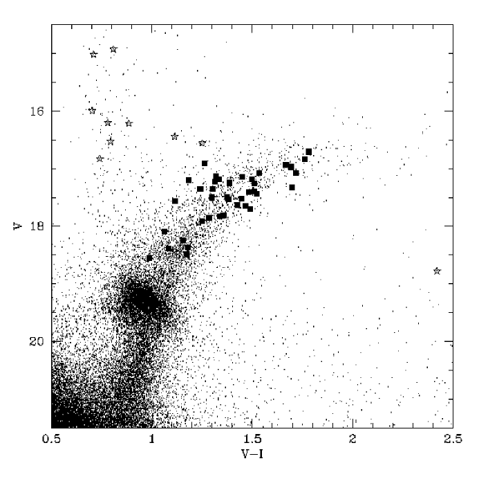
Figure 1: CMD of the Disk 1 field obtained from the CTIO 1.5m telescope. 39 LMC member giants for which abundance measurements were made are marked with solid squares. Excluded foreground stars are marked as open stars, as is star 36, afflicted with strong TiO lines.

The bona fide LMC giants are listed in Table 1. Thirty-eight of the targets were easily matched to stars in the USNO-A astrometric reference catalog (Monet, 1998), and for these stars the USNO number and coordinates are given in columns 2–4. Columns 5 and 6 give the summed equivalent width of the two strongest lines of the Ca II triplet and the associated 1-$\sigma$ error, in Ångstroms; columns 7 and 8 give the V magnitide and error of each star, from Cole (1999); columns 9 and 10 respectively list the metallicity of the star according to the calibration in §2.3, and the random error associated with the metallicity value. Column 11 divides the sample of red giants into four subgroups for further analysis. Group i stars lie fainter than 18th magnitude; group ii stars are brighter than V = 18 and bluer than V$-$I = 1.6; group iii stars lie between V$-$I = 1.6 and 1.85. Additionally, five of the bluest stars in selected magnitude ranges are classed into group iv. These subdivisions will be discussed further in §2.4 below. Star 36, strongly affected by TiO lines, is excluded from further analysis.

Our selected targets span the width of the RGB in the magnitude range 16.7 $\leq$ V $\leq$ 18.5. The distribution of targets in the CMD is shown in Figure 1. Our selection process should not strongly bias our sample against the detection of metal-poor stars; comparison to globular cluster fiducial giant branches (Da Costa & Armandroff, 1990) shows that roughly one-third of our RGB sample lies to the blue of the [Fe/H] = $-$1 globular cluster fiducial sequence.

In order to calibrate our metallicity scale to the system of (Rutledge et al. 1997a, , b), we also oberved a sample of giants and red clump stars in five Galactic globular clusters and the open cluster M67. The clusters span a factor of $\sim$3 in age, and two orders of magnitude in heavy element abundance. The clusters, their horizontal branch magnitudes, abundances, and calcium enhancements are given in Table 2. The individual calibrator stars, magnitudes, and equivalent widths are given in Table The Metallicity Distribution Function of Red Giants in the LMC ; exposure times ranged from 30–300 seconds.

Bias exposures and dome flats were taken at the start of each night; sky exposures to correct for fringing in the CCD were taken during evening and twilight. We observed the 13th magnitude B1 supergiant Sk $-$71$\arcdeg$ 11 on night 1 in order to estimate the effect of telluric absorption lines on a relatively featureless spectrum. Because the data were taken during bright time, through clouds, every spectrum included Ca II lines from the reflected and scattered sunlight. However, we found that all atmospheric and solar features subtracted out cleanly from the region around the redshifted Ca II lines in the LMC target spectra.

The data were reduced with the IRAF ccdproc and ctioslit tasks, using the bias frames, overscan region, dome flats, and sky flats to remove the instrumental signatures from the frames. The sky fringes showed a maximum peak-to-peak relative amplitude of $\approx$6%, and were removed with little difficulty. A number of bad columns were masked off during the reductions, to prevent them from affecting the line identification or measurement procedures.

Because most exposures contained at least two target objects, it was necessary to identify the spectrum of each star interactively. Each spectrum was traced along the dispersion axis, using a linear fit where possible. Near the ends of the slit, it was necessary to use a cubic spline to trace and extract the spectra. The stellar spectra were extracted by interactively fitting a Gaussian shape to the stellar profile across the dispersion direction, placing sky windows appropriately to avoid the wings of neighboring stars and bad pixels. Spectra were extracted using an optimal weighting procedure; the spectra were then rectified using spline fits to selected areas of the continuum that were judged to be unaffected by atmospheric absorption or emission lines.

2.2 Equivalent Widths and Abundances

Rutledge et al. (1997a) summarize the various approaches to measuring the Ca II triplet in the literature. We have followed the procedure of Suntzeff et al. (1993), using Gaussian fits to the line profiles of the two strongest lines of the triplet ($\lambda\lambda$ 8542, 8662 Å). The weakest line is excluded because its inclusion usually decreases the final signal-to-noise of the summed equivalent width measurement (Armandroff & Da Costa, 1991; Rutledge et al. 1997a, ). We followed Suntzeff et al. (1993) and Olszewski et al. (1991) in adopting the continuum bandpasses of Armandroff & Zinn (1988) in our measurements. We used the IRAF task rvidlines to define the wavelength scale of each spectrum, and measured the equivalent widths relative to the near-IR stellar pseudo-continuum using splot. Photometry for the calibration stars was taken from the literature; references are given in Table The Metallicity Distribution Function of Red Giants in the LMC . Photometry for the LMC target stars was taken from our own WFPC2/HST data (Smecker-Hane et al. 1999a, ; Cole, 1999).

The equivalent widths for the calibrating cluster stars are given in Table The Metallicity Distribution Function of Red Giants in the LMC , spanning the range 2.2 $\lesssim$ $\Sigma$W(Ca) $\lesssim$ 6.1. Of the 10 stars in our sample in common with Suntzeff et al. (1993), we find their equivalent widths to be systematically smaller than ours by 1.5%, although this trend is largely masked by the scatter of $\pm$0.22 Å between the two samples. We have 7 calibration stars in common with Olszewski et al. (1991); because they included the $\lambda$8498 line in their measurements, their equivalent widths are 26% larger than ours, with a scatter of $\pm$0.09 Å around the mean relation. Our calibration sample only contained two stars in common with Rutledge et al. (1997a), both in M 68 (NGC 4590). Those authors used a weighted sum of all three triplet lines to compute $\Sigma$W(Ca), where we took a straight sum of the two strongest lines. The Rutledge et al. (1997a) weighting scheme generally assigns a very low weight to the weakest line, and this is reflected by the fact that for the two stars in common, $\Sigma$W(Ca)_R97a = 1.05 $\pm$0.05 $\Sigma$W(Ca)_new. We will show in the next section that we may safely use the Rutledge et al. (1997b) metallicity calibration with our data.

Equivalent widths for the LMC targets are given in Table 1; the red clump of the Disk 1 field is measured to lie at V = 19.26, with a full-width at half-maximum of 0.29 mag (Cole et al., 1999). Because the magnitude error on an individual red clump star is $\approx$0.03 mag, the width of the clump is due to stellar evolutionary effects and the mixture of stellar populations in the field. We consider the possible implications of these variations on our MDF in section 2.4.1.

2.3 Calibrating the $\Sigma$W(Ca)-[Fe/H] Relation

The behavior of $\Sigma$W(Ca) is biparametric with surface gravity and calcium abundance; Rutledge et al. (1997b) describe the procedure for removing the signature of gravity from $\Sigma$W(Ca) in globular clusters. This correction is possible because on the giant branch of a star cluster, there is a one-to-one relation between luminosity and surface gravity: stars along the length of the giant branch have nearly the same mass, but the more highly evolved stars have larger radii and hence lower surface gravity. For low-mass, metal-poor stars, the relation between surface gravity and V magnitude is very close to linear between the level of the horizontal branch and the RGB tip.

An easily measurable surrogate for the difficult-to-measure surface gravity, and the one that is most frequently adopted (Rutledge et al. 1997b, , and references therein), is the difference in magnitude between a target star and the horizontal branch level, V$-$V_HB. Using the V$-$V_HB method, it is possible to reduce the $\Sigma$W(Ca) to a number that depends only on abundance, W^′ (known as the reduced equivalent width). The Rutledge et al. (1997b) result, based on the catalog of Rutledge et al. (1997a) for globular clusters in the approximate range $-$0.3 $\gtrsim$ [Fe/H] $\gtrsim$ $-$2.3, is:

$$\mathrm{W^{\prime}}=\Sigma\mathrm{W(Ca)}+0.64(\pm 0.02)\,(\mathrm{V}-\mathrm{V_{HB}}).$$ (1)

We adopt the abundance scale of Carretta & Gratton (1997), which was shown by Rutledge et al. (1997b) to scale linearly with W^′ according to the relation

$$\mathrm{[Fe/H]_{CG97}}=-2.66+0.42\,\mathrm{W^{\prime}}.$$ (2)

Both the slope and zeropoint of the giant branch relation between log g and M_V are theoretically predicted to depend on age and metallicity (see, e.g., the models of Girardi et al. 2000). Also, it remains uncertain over what range of stellar parameters the linear relations between surface gravity, metallicity, and $\Sigma$W(Ca) hold true (Díaz et al., 1989; Jørgensen et al., 1992). However, the methods espoused by Rutledge et al. (1997b) have been used for targets much more youthful and/or metal-rich than the calibrating globulars with apparent success.

For example, de Freitas Pacheco et al. (1998) obtained integrated optical spectra and V$-$K colors for five interemediate-age LMC clusters (NGC 1783, NGC 1978, NGC 2121, NGC 2173) and three ancient clusters (NGC 1466, NGC 2210, H 11) that had been observed by Olszewski et al. (1991). Within the errors of both methods, the Ca II triplet and the spectral indices yield similar abundances for the ancient clusters, as expected. For the intermediate-age clusters, there is a large scatter between the methods. Because the integrated colors used by de Freitas Pacheco et al. (1998) are susceptible to age-metallicity degeneracy, we shift their measured abundances to the values that would have been obtained if the cluster ages from color-magnitude diagrams had been adopted. We used the relation provided by de Freitas Pacheco et al. (1998), namely $\frac{\partial[Fe/H]}{\partial ln\tau}|_{(V-K)}$ = $-$0.329. Comparison of the abundances derived from the de Freitas Pacheco et al. (1998) paper and those of Olszewski et al. (1991) for four intermediate-age clusters shows that the Ca II triplet values are lower than those derived from spectral indices, but only by 0.1 $\pm$0.2 dex. Despite expectations for the breakdown of the Ca II method at young ages and high abundance, we see reasonable agreement with other methods for ages as young as $\approx$1 Gyr and abundances [Fe/H] $\lesssim$ $-$0.25 dex.

Figure 2: Summed Ca II equivalent widths plotted against V$-$V_HB for stars in our calibrating clusters. For each cluster, the best-fit line with slope 0.64 is shown (see text).

The summed Ca II equivalent widths are plotted as a function of V$-$V_HB for the stars in our calibrating clusters in Figure 2. The best-fit lines of slope 0.64 (from Equation 1) are plotted for each cluster. Extrapolating the lines back to V$-$V_HB = 0, we can derive values for W^′ for the clusters. Although we have used a slightly different technique than Rutledge et al. (1997a) for measuring the summed equivalent width of the calcium triplet, we find essentially identical values of W^′ for the five globular clusters common to the two samples:

$$\mathrm{W^{\prime}}_{new}=1.02\,\mathrm{W^{\prime}}_{R97a}+0.002;$$ (3)

the difference between the Rutledge et al. (1997a) system and our own is much smaller than the mean error of the mean in W^′, which is $\pm$0.11 Å. We can test this by using our values of W^′ to rederive an abundance calibration:

$$\mathrm{[Fe/H]_{CG97}}=-2.656+0.402\,\mathrm{W^{\prime}}.$$ (4)

This is in excellent agreement with Equation 2, showing that the differences in calculation of $\Sigma$W(Ca) will not affect our abundance analysis. Such behavior was also found by Smecker-Hane et al. (1999b), who note that the equivalence will not generally hold true in cases where the instrumental resolution and scattered light properties of the spectra differ strongly from that of the Rutledge et al. (1997a) setup.

Equation 4 was obtained excluding M67 from the fit. According to this fit, M67 should have an abundance of $-$0.3 dex, incompatible with the known [Fe/H] = $-$0.06 $\pm$ 0.07 (Nissen et al., 1987). The discrepancy is understandable because no cluster as metal-rich as [Fe/H] = 0 exists in the calibrating sample of Rutledge et al. (1997a), and theory leads us to expect a breakdown of the linear relation between W^′ and [Fe/H] for clusters of solar abundance (Jørgensen et al., 1992).

Figure 3: Summed Ca II equivalent widths plotted against V$-$V_HB for LMC target stars. A typical errorbar is shown at lower right. Dotted lines show constant [Fe/H], labelled at left. Symbol key to subgroups: $\blacksquare$ = faint; $\circ$ = main; $\blacktriangle$ = tip; $\bullet$ = blue.

The summed Ca II equivalent widths for the LMC target stars are plotted against V$-$V_HB in Figure 3. Errorbars are omitted for clarity, but a typical 1-$\sigma$ error is plotted in the lower right corner. Dotted lines denote isofers derived from equations 1 and 4. The four subgroups of Table 1 are plotted with different symbols. Group i, the faint stars, are solid squares; stars on the main body of the RGB (group ii) are plotted as open circles; the stars near the tip of the RGB (group iii) are closed triangles; and group iv, the bluest stars, are closed circles.

2.4 The Spectroscopic Metallicity Distribution Function

Figure 4: MDF, derived from the Ca II triplet, for 39 LMC red giants. [Fe/H] is calibrated following Rutledge et al. (1997a) to the system of Carretta & Gratton (1997) (see text for details). Labels show true number (N_⋆) and fractional distribution ($\phi_{\star}$). The mean abundance is [Fe/H] = $-$0.642.

The abundance histogram for our spectroscopic sample is shown in Figure 4. The random, 1-$\sigma$ errors for individual stars range from 0.10–0.17 dex, with a mean error of $\pm$0.13 dex. [Fe/H] values and the associated random error for each star are given in Table 1. The sharpness of the peak in the [Fe/H] = $-$0.55 $\pm$0.05 bin of Fig. 4 is partially an artifact of the positioning of the bin edges. The dominant error terms are due to 1) errors in the equivalent width, 2) scatter in the calibration relation, and 3) uncertainty in the location of the red clump. These are random errors and do not take into account systematics due to age or [Ca/Fe] variations.

The median [Fe/H] = $-$0.571 $\pm$0.037, while the mean of the sample is [Fe/H] = $-$0.642 $\pm$0.022. The maximum metallicity is [Fe/H] = $-$0.251 $\pm$0.112, and the most metal-poor star in the spectroscopic sample has [Fe/H] = $-$1.548 $\pm$0.127. The distribution can be characterized by a 1-$\sigma$ dispersion about the mean of $\pm$0.30 dex, or by the locations of the 1st and 3rd quartile points at $-$0.828 dex and $-$0.413 dex, respectively.

Figure 5: Abundance histograms for the three minority subgroups in our sample, with their respective mean abundances. The results bear out theoretical predictions for a correlation of giant branch color with metallicity. The faint subgroup may be more metal-poor than the sample as a whole– see text for discussion.

The abundance distributions in the minority subgroups from Table 1 are plotted in Figure 5. The top panel shows the abundances of the five bluest RGB stars; the mean is 0.2 dex lower than the mean of the sample as a whole. In contrast, the stars near the RGB tip (redder than V$-$I = 1.6) are shown in the middle panel of Fig. 5. Their mean abundance is 0.24 dex higher than the mean of the sample. The lower panel of Figure 5 shows that the giant branch between the red clump and V = 18 contains stars spanning the full range of abundances in this field. The lower mean abundance is not statistically significant, given the small sample size; if such a trend persists to larger spectroscopic samples, then we would be forced to examine the effect of magnitude bias on the derived MDF.

The color-abundance correlation readily lends itself to interpretation in the framework of stellar evolution theory: as expected, the bluer stars are, in general, more metal-poor than the redder stars. Note that this trend can be largely erased for field star samples if the epoch of major star-formation persists for a timescale longer than the typical chemical enrichment timescale (e.g., Aparicio et al. 1996, Da Costa 1998). This is because young, metal-rich red giants can have very similar colors to ancient, metal-poor red giants. The implication from the top two panels of Figure 5 is that a mean age-metallicity relation can well-characterize the evolution of the LMC disk, in this field (c.f., Holtzman et al. 1999).

2.4.1 Corrections to the W^′-[Fe/H] Relation

For better or for worse, the Large Magellanic Cloud is not a globular cluster. While this has proved a boon for studies of stellar evolution and galactic structure, it introduces several complications to the attempted derivation of its metallicity distribution function. The issues of age and $\alpha$-enhancement were discussed in the context of the Ca II triplet by Da Costa & Hatzidimitriou (1998). We consider these, as well as the issue of AGB star contamination, here.

There are known to be a large number of AGB stars present in the LMC field, relative to those in a truly ancient population (e.g., Frogel, Mould & Blanco 1990). We find that synthetic CMDs show that the number of early-AGB stars lying hidden in the broad RGB may be as high as 30% of the total number of RGB$+$AGB stars. The calibration of Ca II equivalent width vs. [Fe/H] is tuned to first-ascent red giants, and so may be systematically biased when applied to an intermediate-age mixture of RGB and AGB stars. We used the NLTE line-formation results of Jørgensen et al. (1992), combined with the theoretical stellar evolution models of Girardi et al. (2000) to model this bias. Among stars of a constant age and metallicity, we calculate that a red giant at given V magnitude will have a Ca II equivalent width $\approx$0.04 Å larger than an AGB star at the same magnitude. This translates directly to an error in [Fe/H] of $-$0.02 dex, much smaller than the typical error in abundance of $\pm$0.1–0.2 dex. Even if a third of our measured stars are AGB stars, the derived mean abundance will be virtually unaffected.

The second possibly serious source of error in our analysis is the use of V$-$V_HB to account for the effect of surface gravity on the Ca II equivalent widths. Because theory predicts an exponentially increasing dependence of $\frac{\partial\Sigma W(Ca)}{\partial logg}$ on [Fe/H] (Jørgensen et al., 1992), this problem will be most severe for the high-metallicity end of our sample, precisely where the cluster sample of Rutledge et al. (1997a) becomes severely incomplete.

We can break down the dependencies of $\Sigma$W(Ca) on various stellar parameters, and it is found that the slope of Equation 2 decreases with increasing metallicity. Additionally, the slope of Equation 1 depends not only on the physics of Ca II line formation, but on the slope of the giant branch. The zeropoint of Equation 2 depends on the surface gravity of an RGB star at the level of the red clump/horizontal branch. Combining the theoretical models of Girardi et al. (2000) and Jørgensen et al. (1992), we find that linear equations like Equations 1 and 2 are appropriate for abundance determinations of old, metal-poor stars; Rutledge et al. (1997a) have observationally shown this to be true for globular clusters. However, for stars approaching solar metallicity, and younger than a few billion years, theory predicts a gradual lessesning of sensitivity of [Fe/H] to $\Sigma$W(Ca), until the Ca II triplet eventually becomes nearly useless as a metallicity indicator above a certain abundance. Because of the gravity-dependence, the exact value of the threshold [Fe/H] depends on the stellar mass, and hence age.

Figure 6: Estimated corrections to the spectroscopic MDF for three different systematic effects. The corrected MDFs are plotted as shaded histograms, on top of the MDF from Fig. 4. The panels show the effects of: a) adding M67 back to the calibrating sample; b) considering the variation of red clump magnitude with age and metallicity; c) considering the difference in [Ca/Fe] between the LMC and the calibrating clusters.

We expect the M67 data to deviate from the Rutledge et al. (1997b) calibration line, and indeed this behavior is seen in Figure 2. If we put aside our theoretical expectations for the moment, and switch to a bilinear calibration of [Fe/H] vs. W^′, including M67 in the new fit, we obtain the MDF shown in Figure 6a. The large equivalent widths of the bright LMC giants have caused their abundances to be shifted upward by $\lesssim$0.5 dex, to nearly twice solar metallicity. Such high values are unprecedented (e.g., Jasniewicz & Thévenin 1994), and clearly show the nonlinear dependence of W^′ on [Fe/H] in this age-metallicity regime. In fact, we have already seen that the Ca II triplet applied to LMC clusters as young as $\approx$ 1 Gyr yields values within $\approx$ 0.1 dex of values determined using spectrophotometric indices (q.v. §2.3). Fortunately, the LMC is not as metal-rich as M67 and so the Ca II triplet retains sensitivity for correspondingly large values of stellar surface gravity (i.e., younger ages). The effect shown in Figure 6a shows an extreme case that certainly does not apply to our data; however the drawing upwards of the high-metallicity half of our sample by $\lesssim$0.1 dex is a real possibility. Therefore, we have undertaken to combine new measurements of the Ca II triplet in open and globular clusters with theoretical stellar atmosphere models to remove this uncertainty from future studies of LMC field stars.

Another way in which age and metallicity influence our analysis is in the identification of V_HB (or V_RC) itself; in a star cluster this is relatively straightforward, but in a composite stellar population, the identification of a specific red giant star with a specific HB (or red clump) level is problematic. The 1-$\sigma$ magnitude width of the red clump in our field is $\pm$0.12 mag, which adds a random error of $\pm$0.03 dex to our abundance determinations. However, the red clump magnitude is expected to vary in a regular way with age and metallicity, and so the use of a mean V_RC for all stars can produce systematic errors.

Figure 7: Variation of zero-age red clump magnitude with age and metallicity, from the theoretical models of Girardi et al. (2000). The thick solid line denotes the predicted M_V, given a sample age-metallicity relationship for the LMC. Dashed lines show the observed M_V (RC) if the distance modulus is assumed to be 18.5, with the 1-$\sigma$ width of $\pm$0.12 mag included.

We show the predicted variation of red clump magnitude as a function of age and abundance in Figure 7; models are from Girardi et al. (2000). The magnitude of the zero-age red clump (ZARC) is shown for simplicity. We have taken the age-metallicity and age-[O/H] relations of Pagel & Tautvaišienė (1998), and derived age-[M/H] relations (Salaris et al., 1993) for comparison to the stellar evolution models of a given abundance. The thick solid line shows the predicted variation of M_V (ZARC) in the LMC disk. For comparison, we show the value of M_V (RC), given our observed value of V_RC = 19.26 $\pm$0.12 and assuming a distance modulus of 18.5 mag, as dashed lines. The agreement with theory is encouraging. Figure 7 shows that, by using an average value of V_HB in our analysis, we may have overestimated the metallicity of both the high- and low-metallicity ends of the MDF, while the stars near the peak of the MDF may have had their abundances underestimated by a small amount.

If a correction for clump magnitude is made, the highest abundance stars are decreased in [Fe/H] by as much as 0.1 dex. The correction does not exceed $\pm$0.03 dex for any star more metal-poor than [Fe/H] $\approx$ $-$0.4 in this model. The “clump neutral” MDF is shown in Figure 6b.

A third potential source of systematic error is the known enhancement of $\alpha$-elements in the calibrating sample of Galactic globular clusters. Column 5 of Table 2 shows the measured [Ca/Fe] ratio for the globulars we have observed. There is a clear anti-correlation of [Ca/Fe] with [Fe/H] (e.g., Gilmore & Wyse 1991; Carney 1996; McWilliam 1997). Tinsley (1979) first explained this trend as a result of the very different timescales for Type II supernovae ($\alpha$ + Fe producers) and Type Ia supernovae (Fe producers). Thus the [$\alpha$/Fe] ratio should be controlled by the relative strength and duration of star-formation epochs vs. quiescent periods in galactic evolution, with additional influence from such factors as could vary the Type Ia/Type II SNe ratio.

If the LMC shared the same $\mathcal{SFH}$ and chemical evolution history as the Milky Way, measuring [Fe/H] from lines of calcium would not pose a problem. However, this is not the case. The present-day LMC is thought to be mildly $\alpha$-deficient relative to the Solar neighborhood (e.g., Hill et al. 1995 find [Ca/Fe] = $+$0.11 for [Fe/H] = $-$0.24), but its [$\alpha$/Fe] ratio is expected to change with age in a non-monotonic way (Pagel & Tautvaišienė, 1998). Because the LMC’s star-formation may have been dominated by an intermediate-age burst (e.g., Stryker 1984), there is likely to be a peak in [$\alpha$/Fe] for stars aged slightly less than the burst age, with lower values for both younger and older ages.

Figure 8: Variation of [Ca/Fe] with [Fe/H] for the calibrating clusters (solid squares), and a model for the LMC (solid line).

We can make a zero-order correction for the effects of varying [Ca/Fe], although this will rest on assumptions about the $\mathcal{SFH}$ and the particulars of the adopted enrichment model. Pagel & Tautvaišienė give a theoretical relation between [Ca/Fe] and [Fe/H], for an $\mathcal{SFH}$ model similar to that proposed by Holtzman et al. (1997). We plot the theoretical [Ca/Fe] vs. [Fe/H] curve (Pagel & Tautvaišienė, 1998) in Figure 8, along with the [Ca/Fe] values from the calibrating clusters. The globular cluster values are included in Table 2; they are taken from Carney (1996) and span the range $+$0.32 $\geq$ [Ca/Fe] $\geq$ $-$0.02 We estimate “calcium neutral” [Fe/H] values by correcting the values inferred from the Rutledge et al. 1997b calibration, according to the difference in [Ca/Fe] between the globular clusters and the LMC model.

The adopted corrections are hidden within a $\pm$0.04 dex scatter, below [Fe/H] $\approx$ $-$1.1; in the range $-$1.1 $\lesssim$ [Fe/H] $\lesssim$ $-$0.55, the correction gradually increases to a value of $-$0.07 dex. Where the few-Gyr “burst” in the LMC’s star-formation rate occurs, the correction jumps to $-$0.17 dex, due to the sudden increase in the Type II SNe rate, and then falls rapidly to negligible values for the most metal-rich stars. The “calcium neutral” MDF is shown in Figure 6c. This figure shows that the discontinuity in [Ca/Fe] at the metallicity of the intermediate-age burst may have caused us to overestimate the metallicity of the upper quartile of our sample. The low-metallicity tail is barely changed, although pulled to slightly lower values by $\lesssim$0.07 dex. The quantitative values of the adopted correction are highly susceptible to systematic error stemming from the exact timing and duration of the burst, but the qualititative behavior, that of strengthening the peak of the MDF at the expense of the high-metallicity component, should be robust. However, the effect is almost certainly hidden within the large scatter of [Ca/Fe] among moderate-metallicity stars in the LMC (Pagel & Tautvaišienė, 1998, and references therein). This scatter is to be expected, because it requires multiple supernovae to enrich a star-forming region to [Fe/H] $\approx$ $-$1. Variations in [$\alpha$/Fe] will likely increase with increasing [Fe/H], an effect which is seen in the population of Galactic globular clusters (Kraft, 1994).

The posible systematic effects on our analysis, and their magnitude, are summarized here:

1. The contamination by AGB stars induces a very small ($\approx$ 0.02 dex) bias to smaller abundance for $\approx$30% of the stars.

2. The stars above [Fe/H] $\approx$ $-$0.4 may be biased too low by up to $\sim$ 0.1 dex due to the nonlinear dependence of [Fe/H] on log g and $\Sigma$W(Ca).

3. The peak of the MDF is probably sharper than observed in Figure 4, and the stars above [Fe/H] $\approx$ $-$0.4 may be biased too high by up to $\approx$ 0.1 dex due to the variation of clump magnitude with age and abundance (note that this effect works against item #2).

4. The peak of the MDF may be much sharper than observed in Figure 4, and the stars above [Fe/H] $\approx$ $-$1 may be biased too high by $\lesssim$0.1 dex, due to the changing ratio of [Ca/Fe]. This systematic is the least well constrained of any, and is probably completely hidden by the scatter in [Ca/Fe] at a given [Fe/H].

5. None of the systematic effects we have noted in this section are capable of populating the low-metallicity tail of the MDF– note the similarity of Figure 6a,b,c for [Fe/H] $\lesssim$ $-$1. This fact will become important in our discussion of spatial variations of the MDF (§4.2).

3 Strömgren Photometry

Intermediate-band photometry represents a useful compromise between the photon-gathering ability of wide bandpass filters, and the increased information contained in a high quality spectrum. The Strömgren system was designed to match bandpass windows to strong and distinctive features of a normal stellar spectrum. In this way, astrophysically meaningful color indices of high utility can be formed (Strömgren, 1963).

For late-type (G–M) stars, the primary Strömgren filters are $v$ ($\bar{\lambda}$ = 4118 Å, $\delta\lambda$ = 146 Å), $b$ ($\bar{\lambda}$ = 4697 Å, $\delta\lambda$ = 196 Å), and $y$ ($\bar{\lambda}$ = 5497 Å, $\delta\lambda$ = 241 Å). The $y$ filter transmits no strong spectral features, and is equivalent to a narrower version of Johnson V. The $b$ filter is placed just longward of the wavelengths where metal-line blanketing becomes important, thus $b-y$ is a good temperature indicator. The $v$ filter lies just longward of the Balmer jump; a stellar spectrum in this wavelength region is rife with metal lines. The strongest photospheric lines in $v$ are due to iron peak elements and cyanogen bands (Bell & Gustafsson, 1978). The index $m_{1}$ $\equiv$ ($v-b$)$-$($b-y$) therefore measures the stellar metal abundance by gauging the depression of $v$-band flux relative to the baseline established by $b-y$ (Strömgren, 1963; Crawford & Barnes, 1970). The existence of CN-anomalous stars presents a possible complication to the use of the Strömgren filters (Anthony-Twarog et al., 1995); the effect is expected to be minor for the LMC field stars (see §3.4.1), but may contribute to a metal-dependent offset between abundances derived from the Ca II triplet and Strömgren photometry (§4.1).

A useful feature of the Strömgren system is that $(\frac{\partial(b-y)}{\partial logg})\mid_{T,z}\;\approx(\frac{\partial m_{1}}{\partial logg})\mid_{T,z}\;\approx 0$
(Bell & Gustafsson, 1978; Grebel & Richtler, 1992; Kurucz, 1999). Because of this fact, abundance estimates using Strömgren colors will be much less susceptible to the dreaded age-metallicity degeneracy. The disadvantage is that we will be forced to subtract the contribution of foreground, Galactic dwarf stars from our color-metallicity plots (§3.4.3). This stands in contrast to a spectroscopic study, where radial velocities serve to reject Galactic interlopers.

Isofers (lines of constant metallicity) in the ($b-y$, $m_{1}$) diagram are well-approximated by straight lines within a certain color range (Bond, 1980). Richtler (1989) derived metallicity calibrations for G–K supergiants in the ($b-y$, $m_{1}$) diagram. The calibration was extended by Grebel & Richtler (1992) to red giants, for the color range 0.4 $\leq$ $b-y$ $\leq$ 1.1, corresponding to a temperature range 3600 K $\lesssim$ T_eff $\lesssim$ 6000. This is well-matched to the temperature range of red clump and red giant stars in the LMC. Because the Grebel & Richtler (1992) calibration was largely based on field stars in the Solar neighborhood, it was only weakly constrained at low abundance; this situation has recently been remedied with observations of globular clusters in the Strömgren system by Hilker (2000). The resulting data have greatly improved the accuracy of the color-metallicity calibration for [Fe/H] $\lesssim$ $-$1.

3.1 Observations, Reductions & Photometry

We obtained Strömgren $vby$ images of four fields in the LMC disk and bar during the nights 1997 Nov. 28 – Dec. 1, using the CTIO 1.5-meter telescope and Cassegrain focus CCD imager. The coordinates of each field, names of nearby star clusters, and references to deep WFPC2 CMD studies are given in Table The Metallicity Distribution Function of Red Giants in the LMC . To emphasize the wide range of environments our study will probe, all four fields are listed, together with their radial distances from the center of the LMC. We will consider only the Disk 1 data for the remainder of this paper, in order to make the comparison of abundances obtained via the Strömgren method to those obtained using the Ca II triplet.

The CCD was a SITe 2048² chip with 24 $\micron$ pixels; in combination with the f/7.5 secondary mirror, this yielded a pixel scale of 0$\farcs$435 pixel^-1 and a field of view 14$\farcm$8 on a side. Four amplifiers were used for faster readouts, which resulted in mild, quadrant-dependent variations in readnoise and gain; the averages were $\sigma_{RN}$ = 1.4 $\pm$0.1 ADU and G_inv = 3.0 $\pm$0.2 e^-1/ADU. The chip specs gave a quoted linearity of 4% at 56000 ADU; tests prior to the observations confirmed this, showing linearity better than 1% to a level of at least 49000 ADU.

Observations were taken during dark time, with new moon occurring near the midpoint of the run. Conditions were photometric throughout, with the exception of the middle third of the last night of the run. The seeing, measured by the FWHM of a 2-dimensional Gaussian fit to the point-spread function of isolated stars, was typically in the range 1$\farcs$3–1$\farcs$4 for $v$ and $y$ images. The image quality in $b$ was frequently $\approx$20% worse than in $vy$. The image quality in long exposures was slightly worse than in the short exposures of photometric standards, and represents a convolution of the true, atmospheric seeing, and tracking errors over the 10–20 minute object exposures. The observing log is given in Table 5.

Photometric standards from the list of Richtler (1990) were observed throughout each night, spanning the range of airmasses encountered in our LMC observations. The total exposure times in in this field were t($v$,$b$,$y$) = (4$\times$1300, 2$\times$1300, 2$\times$1200) seconds. The exposure times were chosen to permit high signal-to-noise photometry for red giants down to the level of the red clump at ($v$,$b$,$y$) $\approx$ (20.7,19.9,19.3).

The images were reduced within IRAF, using standard tasks within the CTIO ared package to correct for the zero level and bias variations of the four-amplifier CCD. The data were flatfielded using dome flats to correct for the pixel-to-pixel response variation and smoothed twilight sky flats to correct for the illumination pattern. Additional processing was performed on exposures shorter than 20 seconds to correct for shutter timing differences across the field (Stetson, 1989).

Photometry was performed using the DAOPHOT/ALLSTAR (Stetson, 1987) suite of Fortran programs, together with ALLFRAME (Stetson, 1994) and associated calibration routines (Stetson 1997, private communication). These programs are designed to make empirical, parametric fits to the point spread function (PSF) of isolated stellar images, find the best-fitting position and amplitude of the PSF of each star in a crowded field, and attempt to remove the stellar flux from the image, in an iterative process. The PSF in our images varied cubically with chip position. We refined our PSF starlist and rederived increasingly accurate PSFs with each iteration, until the residuals in the star-subtracted images were indistinguishable from the intrinsic noise in the images.

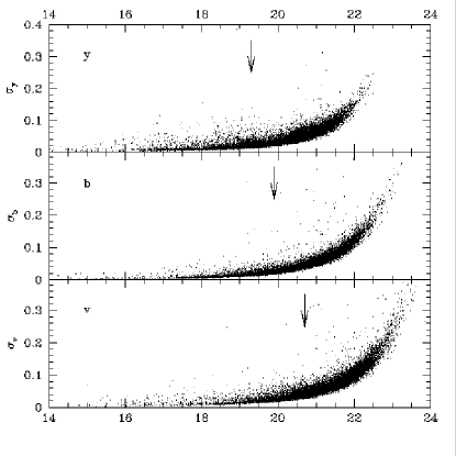
Figure 9: Photometric errors returned by ALLFRAME as a function of stellar magnitude in each Strömgren band. Vertical arrows mark the position of the red clump in each band.

The ALLFRAME program improves upon the precision of measurements derived from a single exposure by simultaneously analyzing the $N$ exposures in different filters and solving for a single ($x,y$) position and $N$ magnitudes per star and the coefficients that describe the geometric transformation between images. The star-subtracted images were then combined into a median image, permitting the identification of faint stars that had previously fallen below the detection threshold. These faint stars were added to the master starlist and ALLFRAME was repeated. This procedure greatly extends the depth and precision of photometry. The final distribution of photometric errors with magnitude for each band is given in Figure 9; for reference, the magnitudes of the red HB clump are marked with arrows.

Stellar magnitudes are computed by the application of aperture corrections based on the measured fluxes of bright, isolated stars in each image; the final magnitudes are intended to represent the best possible approximation to the flux a given star would contribute if it were observed with an infinitely large aperture in an otherwise empty image with zero background. For bright stars, the uncertainty in the aperture correction, $\approx$2–3%, dominates the photon noise.

For calibration we observed stars in the Sk $-$66$\arcdeg$80 (5 stars), NGC 2257 (4 stars), and NGC 330 (6 stars) fields (Richtler, 1990). These stars span the color ranges 0.026 $\leq$ $b-y$ $\leq$ 1.138 and 0.040 $\leq$ $m_{1}$ $\leq$ 0.469. Each star in NGC 330 was measured twice in $vby$ as well as in Johnson V; NGC 2257 was observed three times; because the Sk $-$66$\arcdeg$80 field was located just $\approx$5$\arcdeg$ north of our Disk 1 field, we were able to observe it five times during the night of 1997 Nov 28. We transformed observed colors to the standard system using linear equations for zeropoint, airmass and color terms. The rms scatter of standards about the fit, given here as $\sigma$, was $\approx$1–2%:

$$y=y_{inst}+3.832+0.102\,(b-y)-0.171\,X\,\,\,\,\,\,\,(\sigma=\pm 0.013),$$ (5)

$$b=b_{inst}+4.004+0.173\,(b-y)-0.232\,X\,\,\,\,\,\,\,(\sigma=\pm 0.017),$$ (6)

$$v=v_{inst}+4.438+0.421\,(b-y)-0.326\,X\,\,\,\,\,\,\,(\sigma=\pm 0.020),$$ (7)

The scatter around the calibration line was higher for stars near the western horizon than near the eastern, for a given airmass. An examination of the residuals to our photometric solution indicated a problem with the star Sk $-$66$\arcdeg$82: its measured V magnitude was consistently 1 $\pm$ 0.02 mag brighter than the value given in Table 2 of Richtler (1990). The near-integer offset suggests a typographical error in Richtler’s Table; this was confirmed by comparison to the photometry of Isserstedt (1975), which shows V = 12.8 for this star, rather than 13.8 as reported by Richtler (1990). With this correction, Sk $-$66$\arcdeg$82 agreed perfectly with our calibration relation. Our reduced data are shown in Table 6; column 1 contains an identification number assigned by ALLFRAME, columns 2 and 3 give the positional offsets in arcseconds north and west of the corner of the field, and the photometric quantities $y$, $b-y$, and $m_{1}$, with associated standard errors, fill the remainder of the table.

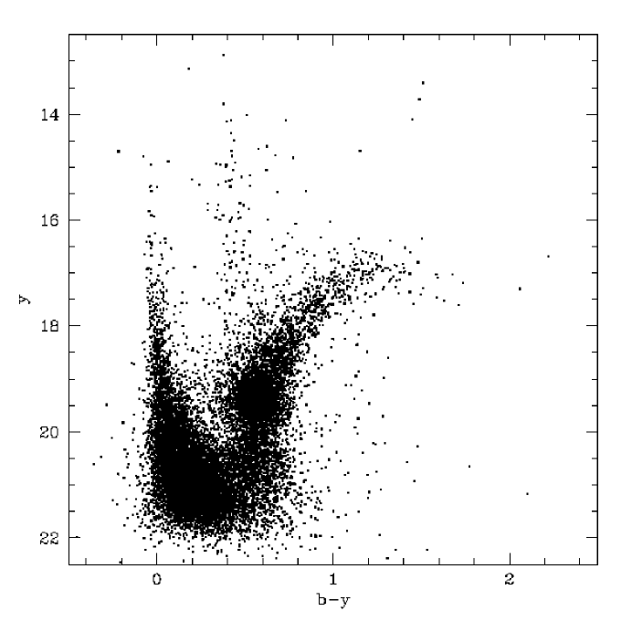
Figure 10: Calibrated ($b-y$, $y$) CMD for 16,958 stars in the Disk 1 field.

The calibrated ($b-y$, $y$) color-magnitude diagram is shown in Figure 10. The CMD shows 16,958 stars in the Disk 1 field, with high completeness down to at least a magnitude below the level of the clump. The highest density of points lies at the red clump, with an extension to fainter, redder magnitudes due to the RGB-bump (as discussed by, e.g., Thomas 1968; Iben 1968; Alves & Sarajedini 1999). The upper giant branch shows the familiar broadening due to the mixture of ages and metallicities in the LMC (e.g., Stryker 1984). Few, if any, luminous AGB stars or horizontal branch stars are present in Fig. 10. The upper main-sequence is prominent for $y$ $\gtrsim$ 17.5, indicating the presence of stars at least as young as 150 million years in this field. The sparse, vertical plume of stars at $b-y$ $\approx$ 0.4–0.5 contains primarily Galactic foreground dwarfs, with a small contribution from blue loop supergiants in the LMC.

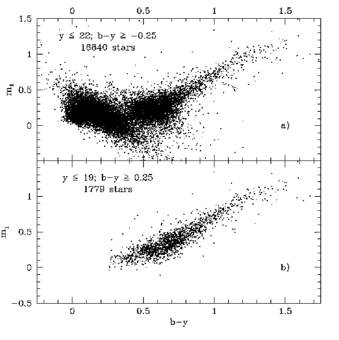
Figure 11: a) The color-metallicity plot (CMP) for the Disk 1 field. b) The CMP, restricted to stars on the upper giant branch, and AGB. These are the stars for which the metallicity calibration of Hilker (2000) is valid.

The ($b-y$, $m_{1}$) plot is shown in Figure 11. This diagram will be referred to as the “color-metallicity plot” (CMP) for the remainder of the paper. The CMP will be the primary tool we use to determine the the chemical abundances of red giant stars. Figure 11a shows the CMP for our main-sequence and red giant stars. Note the narrow width of the giant branch as compared to Figure 10; as described above, age effects are not expected to contribute to the width of the RGB in the ($b-y$, $m_{1}$) plane. Also note the large scatter due to increasing errors for the faintest stars. The error envelope for the red clump stars has the potential to lead to overestimates of the range of abundances contributing to the giant branch MDF. Because increasing photometric errors lead to biased estimates of the range of abundances, we restrict our analysis to the upper giant branch alone; these stars are shown in Figure 11b. For these stars, the calibration of Hilker (2000) is expected to yield accurate abundance estimates (0.5 $\leq$ ($b-y$) $\leq$ 1.1).

3.2 Interstellar Reddening Corrections

Because the determination of metallicities via the CMP relies on a relation between a pair of stellar colors which differ in their sensitivity to interstellar reddening, our results are sensitive both to the total amount of dust along the line of sight and to the form of the reddening curve. Because the $m_{1}$ index is formed from three magnitudes, two of which are blue, its response to interstellar attenuation is especially dependent on the shape of the reddening curve (Crawford & Mandwewala, 1976).

The most commonly cited values for the Strömgren color excesses are based on Crawford & Barnes (1970): E_b-y = 0.74  E_B-V; E_m1 = $-$0.25  E_B-V. These values were based on the Whitford (1958) extinction curve. Although this curve is steeply rising into the violet spectral region, the relatively long wavelength baseline between the $b$ and $y$ filters drives E_m1 to negative values. We thus anticipate a need to “debluen”, rather than deredden, our derived $m_{1}$ indices.

More modern reddening laws (e.g., Cardelli, Clayton & Mathis 1989) show substantially different selective absorption at the wavelength of the $b$ filter than the Whitford (1958) curve; the adoption of a new reddening law requires a recalculation of the Strömgren color excesses. However, the recent literature shows disagreement as to the effect of interstellar reddening on the Strömgren indices. Schlegel et al. (1998) and Fitzpatrick (1999), for example, approximately recover the Crawford & Mandwewala (1976) results: E_b-y = (0.75 $\pm$ 0.02)  E_B-V; E_m1 = ($-$0.25 $\pm$ 0.02)  E_B-V. On the other hand, the model atmosphere grids of Kurucz (1999) show E_b-y = 0.69  E_B-V, an 8% decrease, and E_m1 = $-$0.12  E_B-V, a 50% increase.

Because it was not to clear to us which of these determinations, if any, are correct, we redetermined the Strömgren system color excesses. We convolved theoretical model stellar atmospheres appropriate to slightly metal-poor ([M/H] = $-$0.5) K-type giants (Kurucz, 1999) with the throughput curve of the S2K CCD and the transmission efficiency curves of the CTIO Strömgren filter set. When the resulting spectral energy distribution was convolved with a Cardelli et al. (1989) extinction curve, assuming R_V = 3.1, the results tabulated by Kurucz (1999) were approximately recovered. Our determinations of the Strömgren color excesses are:

$$E_{b-y}=0.70\,E_{B-V}$$ (8)

$$E_{m1}=-0.10\,E_{B-V}.$$ (9)

On the observational side, Delgado et al. (1997) used the Strömgren filter system to observe four highly reddened open clusters. In their reductions, they derived E_b-y = (0.72 $\pm$0.04)  E_B-V, and E_m1 = ($-$0.14 $\pm$0.04)  E_B-V. The scatter is consistent with all published determinations of E_b-y; the observed E_m1 is 1$\sigma$ from our theoretically calculated value, but $>$2.5$\sigma$ from the Schlegel et al. (1998) or Fitzpatrick (1999) values. The difference in spectral energy distribution between the relatively blue stars observed by Delgado et al. (1997) and the cool model atmospheres (Kurucz, 1999) is clearly not the source of the discrepancy between our values for the Strömgren color excesses and those of Schlegel et al. (1998) or Fitzpatrick (1999).

It is uncertain which set of reddening values is more appropriate to observations of the LMC; we adopt our calculated reddening law (Equations 8 and 9). For an assumed reddening E_B-V = 0.10 mag, the derived [M/H] for a given ($b-y$, $m_{1}$) pair will be $+$0.08 dex higher if the Fitzpatrick (1999) values are used for E_b-y and E_m1.

Isofers in the CMP lie nearly perpendicular to the reddening vector, so the derived abundances are highly sensitive to errors in the adopted reddening. For example, a given ($b-y$, $m_{1}$) pair may yield an abundance [M/H] = $-$0.33 if no reddening is assumed, but if dereddened by E_B-V = 0.10 mag, the derived abundance will be solar ([M/H] = 0).

We now turn to the determination of E_B-V itself. Schlegel et al. (1998) give $\langle$E_B-V$\rangle$ = 0.03 for this region of the LMC. This is in good agreement with the mean value for cool stars determined by Zaritsky (1999) for a similar area on the opposite side of the LMC bar. Given the importance of an accurate determination of E_B-V, we used the bright, blue stars in Figure 10 to make an independent reddening determination for the Disk 1 field. We have constructed a reddening-free index for the Strömgren colors based on the relation E_v-b = 0.82  E_b-y. We performed a linear fit to Kurucz model atmospheres for main-sequence stars hotter than ($b-y$)₀ $\leq$ 0.10, and derived

$$(v-b)_{0}=1.78\,(b-y)_{0}+0.173.$$ (10)

If we define the reddening-free index for hot stars

$$Q_{vby}=(v-b)-0.82\,(b-y),$$ (11)

we then obtain the relation

$$(b-y)_{0}=1.04\,Q_{vby}-0.173.$$ (12)

We applied Equation 12 to a sample of 412 stars bluer than $b-y$ = 0.12 and brighter than $y$ = 19 to determine the mean reddening in the Disk 1 field. We find $\langle$E_B-V$\rangle$ = 0.03 $\pm$0.01, with an rms scatter about the mean of $\pm$0.06 mag. This is a very narrow distribution, given the $\approx$4% accuracy of our photometry. Given the low mean value of E_B-V and the almost unresolved scatter about that mean, we are confident that our abundance estimates will not be strongly affected by reddening issues. Our adopted mean reddening values in the Strömgren colors are E_b-y = 0.021, E_m1 = $-$0.003.

3.3 Calibrating the Color-Metallicity Relation

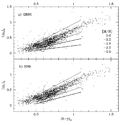
Figure 12: Dereddened CMP for the Disk 1 field. A reddening of $\langle$E_B-V$\rangle$ = 0.03 has been adopted. Isofers from two different calibrations are shown: a) Grebel & Richtler (1992), valid for 0.4 $\leq$ ($b-y$)₀ $\leq$ 1.1; b) Hilker (2000), valid for 0.5 $<$ ($b-y$)₀ $<$ 1.1.

Our technique for using the CMP to derive abundance estimates is based on the observation of Bond (1980) that the slope of the RGB in the CMP is a nearly linear function of [M/H]. This relation was calibrated for metal-rich giants and supergiants by Grebel & Richtler (1992); the calibration was very recently extended to low metallicity by Hilker (2000). In Figure 12 we show our dereddened CMP, with isofers from Grebel & Richtler (1992) overplotted in the top panel, and from Hilker (2000) in the bottom panel. Isofers are plotted at 0.5 dex intervals between 0.0 $\geq$ [M/H] $\geq$ $-$2.0, in both panels. Hilker (2000) quotes a scatter around his mean CMR of $\pm$0.16 dex; this is comparable to the scatter in the Grebel & Richtler (1992) calibration, of $\pm$0.22 dex. These values limit the precision with which the abundance of an individual red giant can be measured using the Strömgren CMP.

The two calibrations agree for solar metallicity, but the Hilker (2000) relation shows a steeper slope for low metallicities. We performed a simple check on the color-metallicity relation (CMR) using stellar evolutionary tracks from the Padua group (Girardi et al., 2000), convolved with model atmosphere grids (Kurucz, 1999) and the CTIO Strömgren filter response functions, for stars of 1 and 2 M_☉. We found that both CMRs match the theoretical tracks for [M/H] $\geq$ $-$0.5, but there is a progressive steepening of the RGB slope as the abundance decreases, which agrees with the steeper CMR of Hilker (2000). The theoretical tracks also start to show deviations from linearity at the blue end of the Grebel & Richtler (1992) calibration for low metallicity, justifying Hilker’s (2000) restriction to ($b-y$)₀ $>$ 0.5. However, for [M/H] $\gtrsim$ $-$0.5, the RGB remains linear at least to the ($b-y$)₀ = 0.4 limit (Grebel & Richtler, 1992). At the red end of the calibration, the theoretical tracks predict that the RGB deviates strongly from linearity for the metal-rich stars, as the $b$-band becomes progressively more swamped by molecular opacity. In the models, this deviation from the linear CMR is seen for solar-metallicity stars cooler than ($b-y$)₀ = 0.9. Such cool, high-abundance stars could possibly account for the group of several stars at ($b-y$)₀ $\approx$ 1.1, ($m_{1}$)₀ $\approx$ 0.5; however the high-metallicity RGB does not appear sufficiently well-populated blueward of ($b-y$)₀ = 0.8 to produce these stars. In general, Figure 12 shows only a mild flattening of the RGB beyond ($b-y$)₀ = 1.1, if any, due to the subsolar metallicity of the LMC field.

An unfortunate property of the Strömgren CMR is the convergence of isofers in the region of the red clump. Where the isofers converge, small errors in photometry and shifts due to differential reddening will lead to huge errors in derived abundance. This effect is stronger in the Grebel & Richtler (1992) CMR, simply because their isofers converge more rapidly at high temperatures. At the level of the red clump, a typical 3% error in $b$ can lead to an abundance error of $\pm$0.84 dex. As the isofers diverge towards cooler temperatures, this becomes a less significant source of error. However, most of the RGB stars lie in the red clump region (see Figure 10); the convergence of isofers is the strongest limitation of the Strömgren CMP for abundance determinations of large samples of stars.

For the remainder of this paper, we adopt the Hilker (2000) color-metallicity relation, because it has been more extensively compared to metal-poor star clusters and provides a somewhat better match to theoretical models for low abundance. The difference between the GR92 and H99 color-metallicity relations is a function of temperature and abundance. For example, at ($b-y$)₀ = 0.5, ($m_{1}$)₀ = 0.25, the difference $\Delta$[M/H]_GR92-H99 = $-$0.20. In contrast, at ($b-y$)₀ = 1.0, ($m_{1}$)₀ = 0.60, $\Delta$[M/H]_GR92-H99 = $+$0.20. For a “typical” star in our Disk 1 field, at ($b-y$)₀ $\approx$ 0.65 and ($m_{1}$)₀ $\approx$ 0.4, the difference $\Delta$[M/H]_GR92-H99 $\lesssim$ $\pm$0.05, smaller than the typical measurement error of $\approx$ $\pm$ 0.2 dex.

3.4 The Photometric Metallicity Distribution Function

Figure 13: The photometric metallicity distribution function for the Disk 1 field, using the Hilker (2000) color-metallicity relation. The mean [M/H] = $-$0.649 $\pm$0.005 for the 1261 stars in the histogram.

The binned MDF of 1261 red giants in the Disk 1 field is shown in Figure 13. Only stars brighter than $y$ = 19 and redder than $b-y$ = 0.50 have been included in the determination. The MDF is characterized by a broad peak between [M/H] = $-$0.7 and $-$0.4, with a steep fall-off towards higher values and a shallower tail to low abundances. In this respect, we have recaptured the basic features of the spectroscopic MDF. The most probable abundance is [M/H] = $-$0.55 $\pm$0.10, while the mean is [M/H] = $-$0.649 $\pm$ 0.005. The median [M/H] = $-$0.635, while the 1st and 3rd quartile values are $-$0.965 and $-$0.342, respectively. While just 6% of the stars are more metal-poor than [M/H] = $-$1.5, 8% of the stars show abundance above solar. Contamination by Galactic foreground stars may account for most of the super-metal-rich stars (see §3.4.3 below).

The 1$\sigma$ width of the best-fitting Gaussian to the MDF is 0.44 dex. However, a single Gaussian leaves a large residual below [M/H] = $-$1.5 unaccounted for; a much better fit was achieved using two Gaussians, a metal-rich and a metal-poor component. A bimodal MDF is reasonable, considering determinations based on star clusters (Olszewski et al., 1991). The metal-rich component, containing 92% of the stars, has a mean [M/H] = $-$0.625 $\pm$0.011 with a 1$\sigma$ width of 0.42 dex. The metal-poor component accounts for the remaining 8% of the stars, with mean [M/H] = $-$1.64 $\pm$0.09 and $\sigma$ = 0.29 dex. The width of the metal-rich component is much greater than that expected from random errors; that of the metal-poor component is less well-resolved.

If we had adopted the Grebel & Richtler CMR, the mean [M/H] would have been shifted downward to $-$0.677 $\pm$0.006, with a more sharply peaked distribution around [M/H] = $-$0.35. The locations of the quartile points, were changed by $\approx$0.03 dex, and the fraction of stars above [M/H] = 0 or below [M/H] = $-$1.5 were unchanged.

3.4.1 The Effect of CN-Anomalous Stars

A drawback of the Strömgren $m_{1}$ index is its sensitivity to variations in CN abundance (Bell & Gustafsson, 1978). CN can even dominate [Fe/H] in determining the $m_{1}$ of globular cluster giants (Anthony-Twarog et al., 1995). In metal-poor globulars, a wide variation in CN strengths is often seen for nearly constant [Fe/H]; the CN-strength distribution function is often bimodal (Kraft, 1994; Anthony-Twarog et al., 1995). Such a bimodal distribution of CN strengths could be invoked to explain the possible secondary component of our photometric Disk 1 MDF, with the majority of the stars populating the CN-strong peak. Without high-resolution spectra, it is impossible to evaluate this hypothesis conclusively.

Because of the multiple dredge-up episodes that RGB and AGB stars undergo, the CN abundances in planetary nebulae have not fully constrained the patterns of CN variation in the still-evolving RGB stars of the LMC field (Dopita et al., 1997). We note that the stars in our field star sample, less massive than 4 M_☉ and less luminous than the tip of the red giant branch, have experienced neither 2nd (Renzini & Voli, 1981) nor 3rd (Girardi et al., 2000) dredge-up events. However, their CN abundances may have been altered by the 1st dredge-up episode, and/or subsequent “extra” mixing (Charbonnel, 1994).

While CN variations may contribute to the width of Figure 13, we doubt that this effect is capable of shifting stars from the primary peak at [M/H] $\approx$ $-$0.5 into the secondary peak at [M/H] $\approx$ $-$1.6. Figure 7 of Kraft’s (1994) review indicates that the separation between CN-strong and CN-weak peaks in a given globular cluster are less than $\approx$0.5 dex, rather than the $\approx$1 dex separation between the two peaks in our Figure 13. Additionally, mildly metal-poor stars ([Fe/H] $\gtrsim$ $-$1) in the Galaxy show far less variation in CN strengh than do the more metal-deficient stars (Kraft, 1994). Studies of old Galactic open clusters have found very little evidence for variations of CN strengths within a given cluster (Janes & Smith, 1984; Janes, 1984). Most of the LMC disk stars are closer in age and abundance to the open clusters than the globulars, but we cannot yet with certainty rule out CN anomalies as a cause of structure in the MDF. In section 4 below, we show that there is evidence that the metal-poor tail of Figure 13 may in fact be stars with [Fe/H] $\approx$ $-$1 that are relatively weak in CN.

3.4.2 Differential Reddening

Differential reddening is expected to be very small in our Disk 1 field, based on 2MASS color-color plots (Nikolaev & Weinberg, 2000). This confirms expectations based on inspection of the H I aperture synthesis maps of Kim et al. (1998), which show our field to be relatively lacking in small-scale structure in the neutral ISM. While differential reddening is expected to be a minor effect for the Disk 1 field in general, it may have a strong effect on the measurements of individual stars. Many LMC red giants suffer essentially zero reddening (Zaritsky, 1999); if they are erroneously dereddened by E_B-V = 0.03 mag, the resulting [M/H] measurement will be in error by $+$0.12 dex, on average. Similarly, the distribution of observed reddening values shows a tail to high (A_V $\gtrsim$ 1) values; a star obscured to such a degree would have its abundance underestimated by $\sim$1.3 dex, i.e., a factor of 20. Clearly the use of the color-metallicity plot should not be relied upon for accurate abundance measurements of individual stars unless independent reddening information is also available. However, insofar as most stars in the field are lightly reddened by an average E_B-V, the Strömgren CMR will yield an accurate value of the mean abundance.

3.4.3 Subtracting the Foreground Dwarfs

Because the Strömgren CMP contains no leverage on surface gravity, our photometric MDF is contaminated by late-type, main-sequence stars in the Galactic foreground. The dominant foreground population is the vertical plume of old stars at the main-sequence turnoff corresponding to the age of the (thick) disk (9–11 Gyr: e.g, Morell et al. 1992). These stars can be seen in Figure 10 at $b-y$ $\approx$ 0.4, the color expected for G-type dwarfs (Crawford & Barnes, 1970). These stars mainly lie to the blue of the area we analyze, and thus only weakly contaminate our photometric MDF.

Cooler foreground dwarfs lie in a tenuous veil across the CMD redward of $b-y$ = 0.4, out to the bottom of the main-sequence somewhere in the vicinity of $b-y$ = 1.3. Their numbers increase dramatically towards fainter magnitudes (Allen, 1973; Bahcall & Soneira, 1980). In order to estimate the level of contamination of the MDF by late-type dwarfs, we compared starcounts in Figure 10 to the predictions of Ratnatunga & Bahcall (1985). Their model predicts that 55, or $\approx$4.4% of the stars that went into our determination of the MDF, are foreground K–M dwarfs.

The Ratnatunga & Bahcall (1985) starcounts are based on the model of Bahcall & Soneira (1980), which is highly smoothed relative to the real, clumpy distribution of stars on the sky; hence variations of a factor of a few from the model predictions are not uncommon. We can scale Ratnatunga & Bahcall’s (1985) prediction to the observed foreground stellar distribution by examining the stars brighter than $y$ = 16.5 and redder than $b-y$ = 0.1, where the contribution of bona fide LMC giants is expected to be negligible. For $y$ $\leq$ 15, where the model predicts 12.5 foreground stars, we count 20, a 60% excess that is only expected to occur by chance in 1.3% of trials. If we include stars down to $y$ $\leq$ 16.5, we count 62 stars where 39.5 are predicted, also a 60% excess. The probability P(62;39.5) = 0.02%, from Poisson statistics; therefore we conclude there is a highly significant excess of foreground stars above the Ratnatunga & Bahcall (1985) prediction. We would then expect nearly 90 contaminators in our photometric MDF, some 7% of the sample.

To subtract the foreground contaminators from the MDF, it is necessary to assume a statistical form for the MDF of the Galactic disk. Wyse & Gilmore (1995) give the combined MDF of the thin and thick disk, showing that it peaks near [M/H] = $-$0.2, with a range of $-$1.4 $\lesssim$ [M/H] $\lesssim$ $+$0.2. Convolving the intrinsic MDF of the thin$+$thick disk from Table 3 of Wyse & Gilmore (1995) with the $\pm$0.16 scatter about the color-metallicity relation, we expect to observe $\approx$15 foreground stars more metal-rich than [M/H] = 0; most of the genuinely super metal-rich stars in our MDF (as opposed to normal stars that appear super metal-rich due to photometric error) are likely to be foreground dwarfs.

The mean [M/H] of a sample of stars drawn from the Wyse & Gilmore (1995) MDF is $\approx$ $-$0.33; subtracting these stars from Figure 13 shifts the mean [M/H] to $-$0.675 (a shift of $-$0.026 dex), does not affect the 1st quartile point, and shifts the 3rd quartile point downward by $-$0.07 dex, to $-$0.41.

4 Discussion

4.1 The Metallicity Distribution Function of LMC Red Giants

The problem with the schemes for correcting the uncertainties in our observed spectroscopic MDF is that they themselves rest on uncertain assumptions and circular reasoning. In fact, the adoption of a specific prescription to correct for the known systematics of our spectroscopic MDF is likely to introduce more problems than it solves. As an example, our corrections for the fading of the red clump and for the [Ca/Fe] ratio assumed a dispersionless age-metallicity relation; such a thing does not exist, according to deep color-magnitude diagram data (Holtzman et al., 1999). Therefore we consider only the uncorrected metallicity distribution function here. However, we have shown in section 2.4.1 that the main sources of systematic error do not change the basic form of the MDF. Uncertainties in the relative height and width of the $-$0.55 dex peak, and in the value for the high-metallicity cutoff surely remain, at the $\pm$0.1–0.2 dex level. Nevertheless, we have identified the basic features of the MDF with enough certainty to discuss its form and implications.

Figure 14: Comparied of Ca II triplet-derived abundances to Strömgren-derived abundances for 34 stars measured by both techniques. Dotted line: The line of equivalence; dashed line: The best-fit linear relation [Fe/H] = 0.363[M/H] $-$ 0.364. The scatter about the linear fit $\sigma$ = 0.18 dex.

First we compare the MDFs derived from photometry and spectroscopy. The advantage of photometric abundance determinations is the ease with which large numbers of stars can be measured. It is of crucial importance to be able place such measurements on a common scale with spectroscopic studies. Figure 14 compares the abundances derived from the Ca II triplet vs. those derived from Strömgren photometry for the 34 stars for which both types of data were available and which fell within the color range of the Strömgren metallicity calibration (Hilker, 2000). The line of equivalence is shown as a dotted line, along with a dashed line representing a linear, least-squares fit to the data.

In order to gain advantage from the large numbers of stars in photometric samples, the random errors of measurement must exceed any serious systematic errors, thereby allowing the errors in statistical quantities to be reduced by observing many targets. The total random error in the Strömgren measurement is dominated by photometric errors (Poisson noise, aperture correction, transformation error, and crowding error); conservatively (i.e., possibly underestimating the error), these contribute $\approx$ $\pm$0.25 dex to the measurement of an individual star. Variable reddening and scatter in the calibration relation contribute an additional $\pm$0.12 and $\pm$0.16 dex of scatter, respectively, for a total random error of $\sigma$ $\gtrsim$ 0.32 dex. The two main sources of systematic error in the Strömgren MDF are variations in the reddening law and variations in CN on the giant branch; the first of these contributes a maximum error of 0.05 dex, because of the low mean reddening in this field. CN-anomalies are likely to contribute less than $\pm$0.1 dex to the error budget (Janes, 1984). Thus, while systematics cannot be ignored, they are a minority contributor to the total error, and thus the multiplexing advantage of CCD photometry is retained. It is important to note that in very highly reddened fields, for old and metal-poor stars (in which CN-anomalies are large and common), the balance of this equation may tip the other way.

We define the offset between the two abundance measures to be $\Delta\left[\frac{M}{H}\right]$ $\equiv$ [Fe/H]_Ca $-$ [M/H]_vby. The mean value of $\Delta\left[\frac{M}{H}\right]$ is $-$0.03 dex, with a 1-sigma scatter of $\pm$0.31 dex about the line of equivalence. This is well within the range expected given the errors in both techniques. However, the offsets are strongly correlated with metallicity. We find

$$\Delta\left[\frac{M}{H}\right]=0.637\,[M/H]+0.365,$$ (13)

with an rms scatter about the line of just $\pm$0.18 dex. This formula can be used to correct Strömgren-derived abundances in order to place them on approximately the same scale as the higher-precision spectroscopic measurements:

$$[Fe/H]_{Ca}=0.363\,[M/H]_{vby}-0.364.$$ (14)

This is the dashed line shown in Figure 14. The residuals to that fit are uncorrelated with abundance. The reason for the good statistical agreement between the photometric and spectroscopic MDFs is that the large majority of stars in the sample lie near [Fe/H] = $-$0.57, where the difference between the two methods vanishes. Although the scatter at the high-metallicity end of Figure 14 somewhat masks the correlation, we find a linear correlation coefficient between $\Delta\left[\frac{M}{H}\right]$ and [M/H] of $r=0.81$. The scatter at high abundance is due to the systematic uncertainty in the calibration of the Ca II triplet method above [Fe/H] $\approx$ $-$0.5. Additional scatter could be introduced by differential reddening or by variations in CN strength at a given [Fe/H], but is not required to reproduce the data.

The cause of the metal-dependent offset between Strömgren and Ca II triplet abundance scales is unknown. For the few globular clusters measured with both techniques, offsets are present, but are much smaller than that inferred from Figure 14 (e.g., Richtler et al. 1999). Because the globular clusters are much older than the bulk of LMC field stars, age effects may be suspected. However, the Strömgren color-metallicity plot is predicted to be insensitive to age (§3). And although the Ca II triplet is sensitive to surface gravity (Jørgensen et al., 1992), we have shown in §2.4.1 that age effects are likely to be small except for the youngest and most metal-rich stars in our sample, not exceeding 0.1–0.2 dex at the most. The direct calibration of the Ca II abundances to the globular cluster abundance scale makes these values more reliable than the photometric indices, especially below [Fe/H] $\approx$ $-$0.5.

If age effects are discounted, then the source of the discrepancy is likely to lie with abundance ratio anomalies; some process is acting to decrease the (Fe$+$CN)/Ca ratio with decreasing [Fe/H] among the LMC field stars. Figure 8 shows that the chemical evolution model of Pagel & Tautvaišienė (1998) predicts an increasing contribution of calcium to the heavy element fraction as the metallicity decreases. However, two factors militate against this being the sole contributor to $\Delta\left[\frac{M}{H}\right]$: first, the effect is nonlinear with [Fe/H], unlike $\Delta\left[\frac{M}{H}\right]$; and second, the effect is unlikely to exceed 0.1 dex over the metallicity range of interest.

While calcium abundances are unaffected by mixing processes during stellar evolution, carbon and nitrogen abundances may be altered by dredge-up of the products of CNO-burning (Renzini & Voli, 1981). The stars in our spectroscopic sample have all experienced the 1st dredge-up episode, which occurs at the base of the red giant branch and acts to deplete the surface abundance of ¹²C while enhancing ¹⁴N. None of the stars in our spectroscopic sample have been affected by 2nd dredge-up (which acts similarly to 1st dredge-up), or 3rd dredge-up (which strongly enhances ¹²C, the primary product of helium-shell burning). In addition to the dredge-up processes, “extra” mixing may take place in some or all RGB stars, above the RGB-bump; all of our stars lie beyond this point. Both 1st dredge-up and extra mixing are predicted to be functions of metallicity (Charbonnel, 1994; Boothroyd & Sackman, 1999). Thus it may be possible that metallicity-dependent mixing processes are acting to deplete CN more quickly for metal-poor stars than for metal-rich stars, leading to increasingly more positive values of $\Delta\left[\frac{M}{H}\right]$ as [Fe/H] decreases.

Possible support for this can be gleaned from Figure 7 of Dopita et al. (1997), where the abundance ratios of carbon, nitrogen, oxygen, and helium are plotted as functions of [$\alpha$/H] for planetary nebulae. The figure shows that [N/$\alpha$] drops precipitously with [$\alpha$/H]; and that while [C/$\alpha$] rises during the same overall abundance range, most of the increase is due to 3rd dredge up, which does not apply to our stellar sample. In star clusters, it is known that CN abundance is usually correlated with the nitrogen abundance, and anti-correlated with carbon (Smith, 1992, and references therein). The observed drop in final nitrogen abundance with decreasing metallicity suggests that mixing is acting much less efficiently in low-metallicity stars; Smith (1992) showed how inefficient dredge-up of nitrogen would lead to CN-weak stars. The strong drop in [N/$\alpha$] for the Dopita et al. (1997) sample of PNe may indicate that the relatively metal-weak field stars of the LMC are generally CN-weak. However, this result is somewhat at odds with predictions that mixing processes on the upper RGB are much more efficient at lower abundance than at higher abundance (e.g., Boothroyd & Sackmann 1999); this would tend to drive the CN-based abundance measures higher than the Ca-based measures for metal-poor stars, contrary to our observations. To confirm or reject the interpretation of Figure 14 as the result of metallicity-dependent mixing would require high-resolution spectroscopy for detailed abundance analyses, as well as further Strömgren photometry of intermediate-age, metal-poor populations, preferably extending to magnitudes well below the RGB-bump (V $\approx$ 19.4 in the LMC field).

Figure 15: The photometric MDF (figure 13), shown as the shaded histogram. The histogram of photometric abundances, after correction based on the linear fit shown in Figure 14, is shown as the solid line; the best-fit gaussian, with a mean of [M/H]^′ = $-$0.60 and $\sigma$ = 0.20 dex, is shown as a dashed line.

Although its provenance remains uncertain, we can use Equation 14 to shift our photometric MDF (Figure 13) onto the Ca II triplet abundance scale, and to see whether the secondary peak in the photometric MDF is an artifact of the metal-dependent offset between indices. Unfortunately, none of the three stars with [Fe/H]_Ca $<$ $-$1.1 fell into the region with Strömgren photometry, so Equation 14 is not strictly applicable to stars more metal-poor than [M/H] $\approx$ $-$1.7. Still, that range encompasses the peak of the putative metal-poor population discussed in section 3.4. The result of the correction is shown in Figure 15: the uncorrected data are shown as the shaded histogram, while the corrected MDF is shown as the solid-outlined histogram. The effect of the correction is to sharply narrow the distribution; a single Gaussian with mean [M/H]^′ = $-$0.60 and dispersion $\sigma$ = $\pm$0.20 is now a close fit to the data (dashed curve in Figure 15). There remains an excess of high-metallicity stars, attributable to Galactic foreground. The “secondary peak” discussed in §3.4 is much less significant now; adding a second Gaussian to the fit does not improve it significantly, although the amplitude of 8–10% agrees with that derived earlier. However, the mean of this secondary component is now [M/H]^′ = $-$0.93, making it indistinguishable from a slightly extended low-metallicity wing of the main population. It is interesting to note, however, that a second population at [Fe/H] $\approx$ $-$1 is in better agreement with the spectroscopic MDF (Fig. 4) than a population with [Fe/H] $\approx$ $-$1.6 would be. The corrected photometric MDF now seems to underpredict the number of metal-poor stars, compared to the spectroscopic MDF; Strömgren photometry of stars below [Fe/H] = $-$1.1 is needed to address this deficiency.

Because of the uncertainties attending the form of our photometric MDF, we prefer to explore the chemical evolution of the Disk 1 field using our spectroscopic MDF (Figure 4). The shape of our MDF is similar to the MDF of F/G dwarfs in the disk of the Milky Way (e.g., Wyse & Gilmore 1995), shifted to lower values by $\approx$ 0.3–0.4 dex. In this respect, our Disk 1 field closely resembles the disk of the Galaxy in its patterns of chemical enrichment, although this enrichment has been retarded by a factor of $\approx$2 in the smaller galaxy. This pattern apparently extends to the form of the age-metallicity relation, which in the LMC as for the Milky Way seems to have been a mildly increasing function for several Gyr before an abrupt increase during the past 1–3 Gyr (Da Costa, 1991; Edvardsson et al., 1993; Wyse & Gilmore, 1995; Pagel & Tautvaišienė, 1998).

The most metal-rich stars we found in the spectroscopic sample showed [Fe/H] $\approx$ $-$0.25; this is consistent with a cutoff in the photometric sample if the decreased precision and contamination by foreground dwarfs is considered. Because we have measured red giant stars, our MDF does not extend to the youngest stars in the LMC, cutting off at $\sim$500 Myr. If chemical enrichment has proceeded normally during the ensuing timespan, then younger populations should be more metal rich than this limit. This behavior is in fact observed: Hill et al. (1995) find [Fe/H] = $-$0.24 $\pm$0.1 for a sample of F/G supergiants, and Jasniewicz & Thévenin (1994) note similar values for 10–40 Myr-old star clusters. The most metal-rich stars in the LMC are about twice as enriched as the intermediate-age stars measured here, a fact which must be taken into account if these results are to be correctly applied to synthetic CMD analyses.

4.2 Spatial Variations in Stellar Populations

Recent WFPC2 (Geha et al., 1998; Holtzman et al., 1999) and ground-based (Westerlund et al., 1998) studies have suggested that most areas of the LMC disk share a common $\mathcal{SFH}$. This is broadly consistent with a shallow or nonexistent radial metallicity gradient (Olszewski et al., 1991). These studies appear to conflict with the earlier results of Bertelli et al. (1992) and Vallenari et al. (1996), who found evidence from wider-field, but shallower, CMDs for a spatially varying $\mathcal{SFH}$. Most of the differences may be attributable to variations in adopted age-metallicity relation. There is also increasingly strong evidence that the form of the MDF varies spatially (Bica et al., 1999). Those authors examine the spatio-temporo-chemical distributions of star clusters and find that although the radially distant clusters are more metal-poor than the inner clusters, they are also older. For clusters of a given age, Bica et al. (1999) do not find evidence for any metallicity gradient.

This fact has been interpreted as evidence for two distinct populations of star clusters (e.g, Kontizas et al. 1990). In this picture, there is an inner disk, $\approx$8$\arcdeg$ across, embedded within a thicker disk $\approx$ 13$\arcdeg$ $\times$ 10$\arcdeg$ in size. The data of Bica et al. (1999) can be placed within this framework, indicating that the LMC has a spatially compact intermediate-age cluster system and a more diffuse, older system (also see Olszewski 1999).

Figure 16: Our spectroscopic MDF (top panel), compared with that of 36 outer disk field stars from Olszewski (1993; middle panel), and 70 LMC star clusters from Olszewski et al. (1991; bottom panel). The older data have been corrected to the Carretta & Gratton (1997) abundance scale as described in the text. The fraction of stars below [Fe/H] $\approx$ $-$1 is 3 times higher in the outer disk field than in the inner disk field. The field stars of the inner disk lack the extremely metal-poor component represented by the ancient globular clusters, but seem similar to the intermediate-age clusters.

This model for the LMC structure is reminiscent of the “Baade sheet” concept for stellar populations, in which all galaxies support an extended distribution of ancient stars (Hodge, 1989). Do the abundance distributions of field stars support this pattern? Olszewski (1993) presented spectroscopic data, obtained for the Ca II triplet, for 36 red giants in a far northern field of the LMC. Their field was in close proximity to the globular cluster NGC 2257, 8$\fdg$5 northeast of the optical center of the bar (i.e., at 5 times larger radius than our Disk 1 field).

We compare the abundance histogram of Olszewski (1993) to our spectroscopic MDF in Figure 16. Because their results were calibrated to the Zinn & West (1984) abundance scale, we have corrected their histogram bins to the high-dispersion, Carretta & Gratton (1997) scale. This has been achieved using the relations in Rutledge et al. (1997a), for [Fe/H]_ZW $\leq$ $-$0.5, and by taking a constant offset between the two scales for higher abundances.

To within the calibration uncertainties, the two abundance distributions are seen to agree well, above [Fe/H] $\approx$ $-$0.8. Below that level, the difference is striking. The second maximum found at [Fe/H] = $-$1.2 by Olszewski (1993) is reduced to a mere tail in our sample. While one-third of the outer disk sample lies below [Fe/H] = $-$1 (Olszewski, 1993), only 10% of the inner disk sample is so metal-deficient. There are two possible explanations for this. One is that selection effects have either biased us against detection of metal-poor stars, or that Olszewski (1993) were biased in favor of metal-poor stars. Because we chose our target stars from a random sample of colors, it is unlikely that we would have missed such a large fraction of metal-poor stars. Olszewski (1993) included stars well to the blue of the RGB ridgeline in their sample, in an effort to obtain a complete census of metal-poor stars, and so it is quite possible to believe that they more efficiently detected metal-poor stars than we did. However, we examined a color-magnitude diagram of the NGC 2257 field (Testa et al., 1995), and there do not appear to be many cool (metal-rich) red giants that would have been missed in the spectroscopic survey. Olszewski (1993) state that many of their blue targets turned out to be Galactic field stars. Selection bias is therefore unlikely to account for the large difference in MDF between the inner and outer field.

Our preferred explanation for the difference is that we are seeing an effect analogous to that described by Bica et al. (1999) for the star clusters. The intermediate-age, metal-rich stars are more centrally concentrated than the older, metal-poor stars. Hence for a given sample size, the relative fraction of metal-poor stars rises with increasing radius. However, the intermediate-age stars throughout the LMC disk have apparently been enriched to the same level. It is evident that spectroscopic studies of the inner LMC disk must contain $\gtrsim$100 stars if the metal-poor component seen by Olszewski (1993) in the outer disk is to be reliably detected.

The similarity of field stars to star clusters is reinforced by comparison to the cluster abundance study of Olszewski et al (1991). Their abundance histogram has been transformed to the Carretta & Gratton (1997) metallicity scale by the same procedure we applied to the field star data. The two samples are plotted in Figure 16; It is seen that our Disk 1 field, which is dominated by stars with [Fe/H] $\approx$ $-$0.55, resembles the abundance distribution of intermediate-age star clusters. However, a metal-poor, globular cluster-like population is found to be lacking in the inner disk.

Attention is also drawn to the excess numbers of field stars with abundances between $-$1.2 $\leq$ [Fe/H] $\leq$ $-$0.8, relative to the star cluster population. This is direct evidence that the star-formation in the field was not as quiescent as cluster formation, during the 4–12 Gyr age gap, as inferred from WFPC2 color-magnitude diagrams (Gallagher et al., 1999; Holtzman et al., 1999). Although the absolute numbers of stars are small, and hence statistically uncertain, Figure 16 may be taken to support the idea that field star formation did the bulk of the chemical enrichment work in the LMC during the cluster dark ages, as required by the cluster abundance distribution (Olszewski et al., 1996). Larger spectroscopic samples are urgently needed in order to put this result on firmer statistical ground. However, it is already supported by our corrected photometric MDF (Figure 15), which shows an excess of stars at [M/H]^′ $\approx$ $-$0.95 compared to the best-fit Gaussian that matches the majority stellar population.

5 Summary and Future Work

In this paper, we have described the first results of a program to measure the metallicity distribution functions (MDF) of red giant stars in selected LMC fields. The specific fields coincide with regions of deep WFPC2 photometry, so that color-magnitude diagram and abundance information may be coupled to derive an accurate and unique history of star-formation for the bar and disk of the LMC.

The data reported here were taken in a single field of the inner LMC disk, 1$\fdg$8 southwest of the optical center of the bar. Two techniques for the derivation of abundances are employed: medium resolution spectroscopy at the Ca II IR triplet, and intermediate-band photometry in the Strömgren system. Strömgren photometry for the remainder of our WFPC2 fields is in hand, and we plan to obtain much larger spectroscopic samples in forthcoming observing seasons.

The possible effects of systematic errors on the Ca II triplet abundance scale as applied to the LMC were examined. Contamination of the sample by AGB stars was shown to have a negligible effect on our derived MDF. The physics of Ca II line formation suggest that the metal-rich end of our MDF ([Fe/H] $\gtrsim$ $-$0.4 dex) might be biased to low values by $\approx$0.1 dex; however, the observational method to correct for surface gravity effects, based on the magnitude of the horizontal branch (red clump) probably compensates for this to some degree. A potentially large, but unconstrained, source of error is the variation in [Ca/Fe] ratio among LMC stars. However, none of these systematics is expected to greatly affect the metal-poor end of our MDF, which is where the most striking comparison to other work can be made, and where the strongest constraints can be placed on $\mathcal{SFH}$ models.

Systematic effects in the Ca II triplet may change the details of the high-metallicity end of our MDF, but its basic form is robust. However, we note that the Ca II triplet method as it stands should only be applied to intermediate-age and young systems, where [Fe/H] may exceed $-$0.3, with extreme caution. We have embarked on a new study to addess this issue and derive a new calibration of the Ca II triplet from a sample of open and globular clusters.

We consider the effects of interstellar reddening on the Strömgren colors; a wide range of behaviors reported in the literature, and we rederive the reddening relations. Although the mean reddening in our Disk 1 field is small, caution must be exercised in applying the results of Strömgren photometry without careful attention to reddening. Despite this weakness, the insensitivity of Strömgren colors to age makes it the preferred photometric abundance indicator where large age variations are known to be present.

The MDF determined photometrically is in good agreement with our spectroscopic results, although there is a significant offset between the two techniques that is linearly dependent on [M/H]. The scatter in the correlation relation is not larger than predicted based on the random errors in each technique. The origin of this offset should be elucidated by high-resolution spectroscopy, in combination with further photometry of stars on the lower RGB, and for metal-poor stars.

We find that the statistical properties of the spectroscopic MDF are well-preserved in the photometric sample, with the following caveats: 1) foreground stars are an important contributor to the metal-rich wing of the photometric MDF; 2) the scatter of individual measurements about the mean color-metallicity relation must be taken into account when assessing the width of the abundance distribution, and 3) the lack of low-metallicity stars in our spectroscopic sample makes the calibration of Strömgren abundances to the Ca II triplet scale quite uncertain below [Fe/H] $\approx$ $-$1.1. However, insofar as the offset between abundance scales is stable for intermediate-age stars, Strömgren photometry can be an important tool for exploring the MDF of large numbers of stars.

Based primarily on our spectroscopic data, we find the median metallicity of the inner LMC disk to be [Fe/H] = $-$0.57 $\pm$0.04, while the mean [Fe/H] = $-$0.64 $\pm$0.02. The errors are random only, and do not reflect the possibility of systematic errors at the $\pm$0.1–0.2 dex level. There is a tail of metal-poor stars in the spectroscopic MDF that extends down to at least [Fe/H] = $-$1.6; the indentification of this tail with a possible metal-poor component of the photometric MDF, containing $\lesssim$10% of the stars, is not certain. This component of the photometric MDF, when corrected via Equation 14 to the Ca II triplet scale, shows a mean [M/H]^′ = $-$0.93. Larger spectroscopic samples are required to address this issue. The intrinsic dispersion in abundances is high, $\approx$0.25 dex; this likely reflects a range in ages as well as a scatter about the mean age-metallicity relation. Half of the red giants in our Disk 1 field fall in the range $-$0.83 $\leq$ [Fe/H] $\leq$ $-$0.41.

We find strong evidence for a radial variation in the relative fraction of metal-rich and metal-poor stars, by comparison to the work of Olszewski (1993). Their outer field shows 3 times as many metal-poor ([Fe/H] $\leq$ $-$1) stars as the Disk 1 field, although the location of the high-metallicity peak at [Fe/H] $\approx$ $-$0.6 is similar. This is interpreted as supporting a model in which stars of a given age share similar abundances, but the intermediate-age stars are more centrally concentrated than the older stars. This would extend to the field populations a trend previously noted for the star clusters (Bica et al., 1999).

By relative number, the Disk 1 field shows twice as many stars in the range $-$1.3 $\leq$ [Fe/H] $\leq$ $-$0.8 than the star cluster sample studied by Olszewski et al. (1991). This may be direct evidence for the hypothesis that star formation in the field did most of the chemical evolution work in the LMC during the time period from 4–12 Gyr ago (Olszewski et al., 1996; Gallagher et al., 1999). Support for this comes from the photometric MDF, which, while imprecise, shows little evidence for a gap at [M/H] $\sim$ $-$1. More work is needed to confirm this result, due to the small number of stars observed spectroscopically.

Future work will see the application of these results to the detemination of the $\mathcal{SFH}$ of the LMC disk. We have obtained deep WFPC2 photometry for two LMC fields, one in the inner disk and one at the center of the bar (Smecker-Hane et al. 1999a, ). Further data will be obtained for a field at the western end of the bar in STScI Cycle 9. These data will result in the best color-magnitude diagrams ever constructed for an extragalactic system. From these CMDs, we will attempt to derive the $\mathcal{SFH}$ of the LMC bar and disk by quantitative comparison to synthetic CMDs (e.g., Tolstoy & Saha 1996). The data we have obtained here will be used to place additional conditions on the synthetic CMDs: not only must the “best fit” model match the observed distribution of points in color and magnitude, we will require that the synthetic MDF also matches the observed one. A full analysis of our WFPC2 CMDs, which contain an order of magnitude more stars than similar data in the literature, will be reported in a forthcoming paper (Smecker-Hane et al., 2000).

Table 1: Identification of Program Stars

ID	Number	$\alpha$	$\delta$	$\Sigma$W(Ca)	$\sigma$W	V	$\sigma$V	[Fe/H]	$\sigma$[Fe/H]	Subgroup
		(J2000.0)	(J2000.0)	(Å)	(Å)	(mag)	(mag)	(dex)	(dex)
1	0150-02697287	05:11:35.934	-71:13:32.49	5.978	0.289	17.133	0.012	-0.792	0.140	ii
2	0150-02699460	05:11:40.558	-71:13:32.63	5.541	0.233	17.632	0.007	-0.843	0.122	ii
3	0150-02677898	05:10:56.610	-71:16:42.30	5.742	0.230	17.808	0.007	-0.719	0.121	ii
4	0150-02701335	05:11:44.596	-71:07:18.21	7.317	0.284	17.144	0.006	-0.251	0.138	ii
5	0150-02701911	05:11:45.833	-71:07:31.69	7.185	0.251	16.707	0.006	-0.413	0.128	iii
8	0150-02692129	05:11:24.810	-71:16:25.77	6.450	0.261	17.909	0.011	-0.409	0.131	ii
9	0150-02691174	05:11:22.924	-71:16:59.02	7.106	0.280	17.410	0.008	-0.270	0.137	ii
10	0150-02690283	05:11:21.244	-71:17:20.87	5.759	0.247	17.205	0.017	-0.862	0.127	iv
11	0150-02689820	05:11:20.342	-71:17:34.68	6.906	0.283	17.437	0.009	-0.343	0.138	ii
13	0150-02686676	05:11:14.372	-71:18:58.24	6.180	0.265	17.260	0.011	-0.679	0.132	ii
15	0150-02684855	05:11:10.930	-71:14:30.44	6.662	0.205	17.398	0.010	-0.451	0.114	ii
16	0150-02682408	05:11:06.094	-71:14:48.70	6.292	0.253	17.702	0.010	-0.524	0.128	ii
17	0150-02679627	05:11:00.480	-71:15:09.98	5.211	0.243	18.383	0.039	-0.789	0.126	i
18	0150-02676927	05:10:54.463	-71:15:33.72	5.497	0.234	18.091	0.006	-0.747	0.122	i
19	0150-02655815	05:10:06.601	-71:15:50.91	6.432	0.257	17.188	0.005	-0.596	0.130	ii
20	0150-02655172	05:10:05.348	-71:15:29.88	6.592	0.287	17.230	0.005	-0.521	0.139	ii
21	0150-02654809	05:10:04.592	-71:15:13.82	6.406	0.245	17.356	0.006	-0.564	0.126	ii
23	0150-02716108	05:12:16.561	-71:08:56.01	3.957	0.249	17.358	0.022	-1.548	0.127	ii
24	0150-02715410	05:12:15.075	-71:08:35.74	4.461	0.206	17.561	0.022	-1.295	0.114	iv
25	$\cdots$	05:12:10	-71:07:33	4.357	0.173	18.491	0.023	-1.105	0.105	i
26	0150-02711752	05:12:07.264	-71:06:56.33	6.582	0.254	18.244	0.022	-0.272	0.129	i
29	0150-02680078	05:11:01.504	-71:14:37.22	4.617	0.378	18.548	0.006	-0.987	0.171	i,iv
30	$\cdots$	05:11:03	-71:14:18	6.009	0.244	17.517	0.012	-0.684	0.126	ii
31	0150-02681765	05:11:04.802	-71:13:49.78	5.753	0.253	18.377	0.007	-0.573	0.128	i,iv
33	0150-02707271	05:11:57.508	-71:09:09.61	6.096	0.249	17.830	0.018	-0.571	0.127	ii
35	0150-02702958	05:11:48.130	-71:12:16.18	5.232	0.240	17.858	0.019	-0.911	0.124	ii
36	0150-02698027	05:11:37.565	-71:12:29.08	3.135	0.261	18.778	0.006	$\cdots$	$\cdots$	TiO
37	0150-02696795	05:11:34.945	-71:12:30.62	5.371	0.264	17.534	0.007	-0.936	0.132	ii
38	0150-02694661	05:11:30.385	-71:12:35.73	6.707	0.291	16.969	0.006	-0.540	0.141	iii
39	0150-02658835	05:10:12.748	-71:10:28.32	5.820	0.254	17.497	0.005	-0.765	0.129	ii
40	0150-02658096	05:10:11.254	-71:10:16.82	6.812	0.258	17.651	0.005	-0.328	0.130	ii
41	0150-02656626	05:10:08.289	-71:09:58.03	5.229	0.299	17.191	0.005	-1.079	0.143	ii
42	0150-02665754	05:10:27.883	-71:18:59.64	7.343	0.199	17.074	0.006	-0.258	0.112	iii
44	0150-02646913	05:09:47.376	-71:14:11.09	7.103	0.277	16.840	0.005	-0.413	0.136	iii
45	0150-02648095	05:09:50.039	-71:13:36.77	6.763	0.233	17.500	0.005	-0.385	0.122	ii
46	0150-02717484	05:12:19.480	-71:19:56.67	6.837	0.226	16.903	0.022	-0.504	0.120	iv
47	0150-02715689	05:12:15.655	-71:19:55.29	6.704	0.266	17.248	0.021	-0.472	0.133	ii
49	0150-02689598	05:11:19.900	-71:16:39.58	7.017	0.254	16.936	0.013	-0.423	0.129	iii
50	0150-02687605	05:11:16.096	-71:16:40.23	6.889	0.222	17.324	0.009	-0.378	0.119	iii
51	0150-02685571	05:11:12.266	-71:16:39.77	5.921	0.279	17.080	0.009	-0.828	0.137	ii

No match found in USNO-A catalog within 2$\arcsec$.

Note. — ID numbers and coordinates are taken from the USNO-A astrometric reference catalog (Monet, 1998), except where noted. Magnitudes are from Cole (1999). For subgroup definitions, see text. Star 36 is excluded from the abundance analysis because of contamination by TiO bands.

Table 2: Calibrating Clusters

Cluster	VHB	[Fe/H]ZW84	[Fe/H]CG97	[Ca/Fe]
M 68 (NGC 4590)	15.68	$-$2.09 $\pm$0.11	$-$2.00 $\pm$0.03	$+$0.32
NGC 1904	16.15	$-$1.68 $\pm$0.09	$-$1.37 $\pm$0.05	$+$0.30
NGC 288	15.30	$-$1.40 $\pm$0.12	$-$1.14 $\pm$0.03	$+$0.12
NGC 1851	16.09	$-$1.33 $\pm$0.09	$-$1.03 $\pm$0.06	$+$0.03
47 Tuc (NGC 104)	14.06	$-$0.71 $\pm$0.08	$-$0.78 $\pm$0.02	$-$0.02
M 67 (NGC 2682)	10.56	$-$0.06 $\pm$0.07		0.00

Note. — Horizontal branch magnitudes from the online catalog of Harris (1996), except as noted. [Fe/H] values from Zinn & West (1984) and Carretta & Gratton (1997), except as noted. [Ca/Fe] values from Carney (1996).

Table 3: Calibrator Magnitudes and Equivalent Widths

Star	V$-$VHB (mag)	$\Sigma$W(Ca)   (Å)	Notes
M 68 / I-74	$-$1.01	2.178 $\pm$0.108	1,2
M 68 / I-256	$-$2.96	3.265 $\pm$0.149	1,2
M 68 / II-28	$-$1.88	2.715 $\pm$0.134	1,2
NGC 1904 / 006	$-$0.89	4.113 $\pm$0.164	2,3
NGC 1904 / 015	$-$2.97	5.281 $\pm$0.164	3,4
NGC 1904 / 089	$-$1.49	4.408 $\pm$0.133	2,3
NGC 1904 / 240	$-$2.20	4.833 $\pm$0.171	3,4
NGC 1904 / 241	$-$2.58	4.818 $\pm$0.144	3,4
NGC 288 / C20	$-$2.30	5.109 $\pm$0.173	2,5
NGC 288 / C23	$-$0.32	3.954 $\pm$0.149	2,5
NGC 288 / C36	$-$1.43	4.357 $\pm$0.194	2,5
NGC 288 / C41	$-$0.82	4.299 $\pm$0.190	2,5
NGC 1851 / 109	$-$1.17	4.725 $\pm$0.187	6,7
NGC 1851 / 112	$-$2.22	5.640 $\pm$0.165	6,8
NGC 1851 / 293	$-$0.59	4.705 $\pm$0.296	6,7
NGC 1851 / 294	$-$2.61	5.886 $\pm$0.137	6,9
NGC 1851 / 333	$-$2.01	5.453 $\pm$0.114	6,8
47 Tuc / L1523	$-$0.09	4.488 $\pm$0.233	10,11
47 Tuc / L2506	$-$0.00	4.787 $\pm$0.214	10,11
47 Tuc / L2514	$+$0.02	4.442 $\pm$0.147	10,11
47 Tuc / L5406	$-$1.23	5.275 $\pm$0.227	9,10
47 Tuc / L5422	$-$1.59	5.545 $\pm$0.156	9,10
M 67 / F84	$+$0.04	5.790 $\pm$0.199	12,13
M 67 / F105	$-$0.23	5.700 $\pm$0.162	12,13
M 67 / F108	$-$0.83	6.092 $\pm$0.166	12,13
M 67 / F141	$-$0.09	5.843 $\pm$0.149	12,13
M 67 / F170	$-$0.83	5.943 $\pm$0.223	12,13

References. — (1) Identification from Harris 1975; (2) Photometry from Suntzeff et al. 1993; (3) ID: Stetson & Harris 1977; (4) Photometry: Stetson & Harris 1977; (5) ID: Cannon 1974; (6) ID: Stetson 1981; (7) Photometry: Stetson 1981; (8) Photometry: Armandroff & Da Costa 1991; (9) Photometry: Da Costa & Armandroff 1995; (10) ID: Lee 1977; (11) Photometry: Lee 1977; (12) ID: Johnson & Sandage 1955; (13) Photometry: Janes & Smith 1984.

Table 4: Selected LMC Fields

Field	$\alpha$ (J2000.0)	$\delta$ (J2000.0)	$\rho$   (deg.)	Notes	References
Disk 1 A$+$B	5:10:50	$-$71:13:31	1.8	Inner disk, near SL336	1,2
HST-1	5:14:44	$-$65:17:43	4.5	Outer disk, near NGC 1866	3,4,5,6,7
HST-2	5:23:51	$-$69:49:28	0.1	Bar, near HS-275	1,2,7
HST-3	5:58:21	$-$68:21:19	3.4	Outer disk, near Hodge 10	6,7

References. — WFPC2 color-magnitude diagram studies: (1) Smecker-Hane et al. 1999; (2) Cole et al. 1999; (3) Gallagher et al. 1996; (4) Holtzman et al. 1997; (5) Stappers et al. 1997; (6) Geha et al. 1998; (7) Holtzman et al. 1999.

Table 5: Catalog of Photometric Observations

Field	Date	Seeing (arcsec)	Exposures
Disk 1A	1997 Nov 28	1$\farcs$4	1200s $y$
Disk 1A	1997 Nov 28	1$\farcs$9	1300s $b$
Disk 1A	1997 Nov 28	1$\farcs$5	2$\times$ 1300s $v$
Disk 1A	1997 Nov 28	1$\farcs$4	1300s $v$
Disk 1A	1997 Nov 28	1$\farcs$6	1300s $b$
Disk 1A	1997 Nov 28	1$\farcs$3	1200s $y$
Disk 1A	1997 Dec 1	1$\farcs$4	1300s $v$

Table 6: Strömgren Photometry of the Disk 1A Field

ID	$\Delta\delta$ ($\arcsec$)	$\Delta\alpha$ ($\arcsec$)	$y$	$\sigma_{y}$	$b-y$	$\sigma_{by}$	$m_{1}$	$\sigma_{m1}$
200001	$-$0.274	388.203	20.184	1.444	0.182	1.865	$-$0.021	2.360
201648	$-$0.083	165.561	19.059	0.287	0.889	0.362	0.206	0.457
201495	0.000	149.296	19.550	0.154	0.219	0.196	$-$0.020	0.249
202309	0.078	264.597	19.607	0.043	0.176	0.063	0.157	0.092
32523	0.087	147.713	19.256	0.031	0.498	0.050	0.300	0.079

References

- Allen (1973) Allen, C.W. 1973, “Astrophysical Quantities”, 3rd. ed. (London: Athlone Press)
- Alves & Sarajedini (1999) Alves, D.R. & Sarajedini, A. 1999, ApJ, 511, 225
- Anthony-Twarog et al. (1995) Anthony-Twarog, B.J., Twarog, B.A., & Craig, J. 1995, PASP, 107, 32
- Aparicio et al. (1996) Aparicio, A., Gallart, C., Chiosi, C., & Bertelli, G. 1996, ApJ, 469, L97
- Armandroff & Zinn (1988) Armandroff, T.E., & Zinn, R. 1988, AJ, 96, 92
- Armandroff & Da Costa (1991) Armandroff, T.E., & Da Costa, G.S. 1991, AJ, 101, 1329
- Baade (1963) Baade, W. 1963, “Evolution of Stars and Galaxies”, ed. C. Payne-Gaposchkin, (Harvard Univ. Pr.: Cambridge)
- Bahcall & Soneira (1980) Bahcall, J.N., & Soneira, R.M. 1980, ApJS, 44, 73
- Bell & Gustafsson (1978) Bell, R.A., & Gustafsson, B. 1978, A&AS, 34, 229
- Bertelli et al. (1992) Bertelli, G., Mateo, M., Chiosi, C., & Bressan, A. 1992, ApJ, 488, 400
- Bica & Alloin (1987) Bica, E., & Alloin, D.M. 1987, A&A, 186, 49
- Bica et al. (1999) Bica, E., Schmitt, H.R., Dutra, C.M., & Oliveira, H.L. 1999, AJ, 117, 238
- Bond (1980) Bond, H.E. 1980, ApJS, 44, 517
- Boothroyd & Sackman (1999) Boothroyd, A.I., & Sackmann, I.-J. 1999, ApJ, 474, 188
- Butcher (1977) Butcher, H. 1977, ApJ, 216, 372
- Cannon (1974) Cannon, R.D. 1974, MNRAS, 167, 551
- Cardelli et al. (1989) Cardelli, J.A., Clayton, G.C., & Mathis, J.S. 1989, ApJ, 345, 245
- Carney (1996) Carney, B.W. 1996, PASP, 108, 900
- Carretta & Gratton (1997) Carretta, E., & Gratton, R.G. 1997, A&AS, 121, 95
- Charbonnel (1994) Charbonnel, C. 1994, A&A, 282, 811
- Cole (1999) Cole, A.A. 1999, Ph.D. Thesis, University of Wisconsin–Madison.
- Cole et al. (1999) Cole, A.A., Smecker-Hane, T.A., & Gallagher, J.S., III 1999, BAAS, #08.15
- Crawford & Barnes (1970) Crawford, D.L., & Barnes, J.V. 1970, AJ, 75, 978
- Crawford & Mandwewala (1976) Crawford, D.L., & Mandwewala, N. 1976, PASP, 88, 917
- Da Costa (1991) Da Costa, G.S. 1991, in IAU Symp. 148, “The Magellanic Clouds”, eds. R. Haynes & D. Milne, (Kluwer: Dordrecht), p. 183
- Da Costa (1998) Da Costa, G.S. 1998, in “Stellar Astrophysics for the Local Group”, eds. A. Aparicio, A. Herrero, & F. Sánchez, (Cambridge: Cambridge Univ. Pr.), p. 351
- Da Costa (1999) Da Costa, G.S. 1999, in IAU Symp. 190, “New Views of the Magellanic Clouds”, eds. Y.-H. Chu, N.B. Suntzeff, J.E. Hesser, & D.A. Bohlender, (San Francisco: PASP), p. 397
- Da Costa & Armandroff (1990) Da Costa, G.S., & Armandroff, T.E. 1990, AJ, 100, 162
- Da Costa & Armandroff (1995) Da Costa, G.S., & Armandroff, T.E. 1995, AJ, 109, 2533
- Da Costa & Hatzidimitriou (1998) Da Costa, G.S., & Hatzidimitriou, D. 1998, AJ, 115, 1934
- de Freitas Pacheco et al. (1998) de Freitas Pacheco, J.A., Barbuy, B., & Idiart, T. 1998, A&A, 332, 19
- Delgado et al. (1997) Delgado, A.J., Alfaro, E.J., & Cabrera-Caño, J. 1997, AJ, 113, 713
- de Vaucoleurs & Freeman (1972) de Vaucouleurs, G., & Freeman, K.C. 1972, Vistas Astron., 14, 163
- Díaz et al. (1989) Díaz, A.I., Terlevich, E., & Terlevich, R. 1989, MNRAS, 239, 325
- Dopita et al. (1997) Dopita, M.A., Vassiliadis, E., et al. 1997, ApJ, 474, 188
- Edvardsson et al. (1993) Edvardsson, B., Andersen, J., Gustaffson, B., Lambert, D.L., Nissen, P.E., & Tomkin, J. 1993, A&A, 275, 101
- Faber & French (1980) Faber, S.M., & French, H.B. 1980, ApJ, 235, 405
- Fitzpatrick (1999) Fitzpatrick, E.L. 1999, PASP, 111, 63
- Frogel et al. (1990) Frogel, J.A., Mould, J.R., & Blanco, V.M. 1990, ApJ, 352, 96
- Gallagher et al. (1996) Gallagher, J.S., III, Mould, J.R., de Feijter, E., Holtzman, J., Stappers, B., Watson, A., Trauger, J., & The WFPC2 IDT 1996, ApJ, 466, 732
- Gallagher et al. (1998) Gallagher, J.S., III, Tolstoy, E., Dohm-Palmer, R.C., Skillman, E.D., Cole, A.A., Hoessel, J.G., Saha, A., & Mateo, M. 1998, AJ, 115, 1869
- Gallagher et al. (1999) Gallagher, J.S., III, Cole, A.A., Holtzman, J.A., & Smecker-Hane, T.A. 1999, in IAU Symp. 190, “New Views of the Magellanic Clouds”, eds. Y.-H. Chu, N.B. Suntzeff, J.E. Hesser, & D.A. Bohlender, (San Francisco: PASP), p. 306
- Gascoigne (1964) Gascoigne, S.C.B. 1964, in IAU-USRI Symp. 20, “The Galaxy and the Magellanic Clouds”, eds. F.J. Kerr & A.W. Rodgers, (Austr. Acad. Sci: Canberra), p. 354
- Geha et al. (1998) Geha, M.C., et al. 1998, AJ, 115, 1045
- Gilmore & Wyse (1991) Gilmore, G., & Wyse, R.F.G. 1991, ApJ, 367, L55
- Girardi et al. (2000) Girardi, L., Bressan, A., Bertelli, G., & Chiosi, C. 2000, A&AS, 141, 371
- Grebel & Richtler (1992) Grebel, E.K., & Richtler, T. 1992, A&A, 253, 359
- Hardy et al. (1984) Hardy, E., Buonanno, R., Corsi, C.E., Janes, K.A., & Schommer, R.A. 1984, ApJ, 278, 592
- Harris (1975) Harris, W.E. 1975, ApJS, 29, 397
- Harris (1996) Harris, W.E. 1996, AJ, 112, 1487
- Hilker (2000) Hilker, M. 1999, A&A, in press, astro-ph/9911387
- Hill et al. (1995) Hill, V., Andrievsky, S., & Spite, M. 1995, A&A, 293, 347
- Hodge (1989) Hodge, P.W. 1989, ARA&A, 27, 139
- Holtzman et al. (1997) Holtzman, J.A., Mould, J.R., Gallagher, J.S., III, Watson, A.M., Grillmair, C.J., & The WFPC2 IDT 1997, AJ, 113, 656
- Holtzman et al. (1999) Holtzman, J.A., Gallagher, J.S., III, Cole, A.A., Mould, J.R., Grillmair, C.J., & The WFPC2 IDT 1999, AJ, 118, 2262
- (56) Holtzman, J.A., Mould, J.R., & Gallagher, J.S., III 1999b, in IAU Symp. 190, “New Views of the Magellanic Clouds”, eds. Y.-H. Chu, N.B. Suntzeff, J.E. Hesser, & D.A. Bohlender, (San Francisco: PASP), p. 306
- Iben (1968) Iben, I., Jr. 1968, Nature, 220, 143
- Isserstedt (1975) Isserstedt, J. 1975, A&AS, 19, 259
- Janes (1984) Janes, K.A. 1984, PASP, 96, 977
- Janes & Smith (1984) Janes, K.A., & Smith, G.H. 1984, AJ, 89, 487
- Jasniewicz & Thévenin (1994) Jasniewicz, G., & Thévenin, F. 1994, A&A, 282, 717
- Johnson & Sandage (1955) Johnson, H.L., & Sandage, A.R. 1955, ApJ, 121, 616
- Jones et al. (1984) Jones, J.E., Alloin, D.M., & Jones, B.J.T. 1984, ApJ, 283, 457
- Jørgensen et al. (1992) Jørgensen, U.G., Carlsson, M., & Johnson, H.R. 1992, A&A, 254, 258
- Kim et al. (1998) Kim, S., Staveley-Smith, L., Dopita, M.A., Freeman, K.C., Sault, R.J., Kesteven, M.J., & McConnell, D. 1998, ApJ, 503, 674
- Kontizas et al. (1990) Kontizas, M., Morgan, D.H., Hatzidimitriou, D., & Kontizas, E. 1990, A&AS, 84 527
- Kraft (1994) Kraft, R.P. 1994, PASP, 106, 553
- Kurucz (1999) Kurucz, R.L. 1999, HiA, 11, 646; http://cfaku5.harvard.edu/grids.html
- Lee (1977) Lee, S.W. 1977, A&AS, 27, 381
- Lehnert et al. (1992) Lehnert, M.D., Bell, R.A., Hesser, J.E., & Oke, J.B. 1992, ApJ, 395, 466
- McWilliam (1997) McWilliam, A. 1997, ARA&A, 35, 503
- Monet (1998) Monet, D.G. 1998, BAAS, 193, #120.03
- Morell et al. (1992) Morell, O., Kallander, D., & Butcher, H.R. 1992, A&A, 259, 543
- Nissen et al. (1987) Nissen, P.E., Twarog, B.A., & Crawford, D.L. 1987, AJ, 93, 634
- Nikolaev & Weinberg (2000) Nikolaev, S., & Weinberg, M.D. 2000, ApJ, submitted, astro-ph/0003012
- Olsen (1999) Olsen, K.A.G. 1999, AJ, 117, 2244
- Olszewski (1993) Olszewski, E.W. 1993, in “The Globular Cluster-Galaxy Connection”, eds. G.H. Smith & J.P. Brodie, (ASP: San Francisco), p. 351
- Olszewksi (1999) Olszewski, E.W. 1999, in IAU Symp. 190, “New Views of the Magellanic Clouds”, eds. Y.-H. Chu, N.B. Suntzeff, J.E. Hesser, & D.A. Bohlender, (PASP, San Francisco), p. 292
- Olszewski et al. (1991) Olszewski, E.W., Schommer, R.A., Suntzeff, N.B., & Harris, H.C. 1991, AJ, 101, 515
- Olszewski et al. (1996) Olszewski, E.W., Suntzeff, N.B., & Mateo, M. 1996, ARA&A, 34, 511
- Pagel & Tautvaišienė (1998) Pagel, B.E.J., & Tautvaišienė, G. 1998, MNRAS, 299, 535
- Ratnatunga & Bahcall (1985) Ratnatunga, K.U., & Bahcall, J.N. 1985, ApJS, 59, 63
- Renzini & Voli (1981) Renzini, A., & Voli, M. 1981, A&A, 94, 175
- Richtler (1989) Richtler, T. 1989, A&A, 211, 199
- Richtler (1990) Richtler, T. 1990, A&AS, 86, 103
- Richtler et al. (1999) Richtler, P., Hilker, M., & Richtler, T. 1999, A&A, 350, 376
- (87) Rutledge, G.A., Hesser, J.E., Stetson, P.B., Mateo, M., Simard, L., Bolte, M., Friel, E., & Copin, Y. 1997a, PASP, 109, 883
- (88) Rutledge, G.A., Hesser, J.E., & Stetson, P.B. 1997b, PASP, 109, 907
- Salaris et al. (1993) Salaris, M., Chieffi, A., & Straneiro, O. 1993, ApJ, 414, 580
- Sarajedini (1998) Sarajedini, A. 1998, AJ, 116, 738
- Sarajedini (1999) Sarajedini, A. 1999, AJ, 118, 2321
- Schlegel et al. (1998) Schlegel, D.J., Finkbeiner, D.P., & Davis, M. 1998, ApJ, 500, 525
- (93) Smecker-Hane, T.A., Gallagher, J.S., III, Cole, A.A., Tolstoy, E., & Stetson, P.B. 1999a, in IAU Symp. 190, “New Views of the Magellanic Clouds”, eds. Y.-H. Chu, N.B. Suntzeff, J.E. Hesser, & D.A. Bohlender, (PASP, San Francisco), p. 343
- (94) Smecker-Hane, T.A., Mandushev, G., Hesser, J.E., Stetson, P.B., Da Costa, G.S., & Hatzidimitriou, D. 1999b, in “The Spectrophotometric Dating of Stars and Galaxies”, eds. I. Hubeny, S. Heap, & R. Cornett, (ASP: San Francisco), p. 159
- Smecker-Hane et al. (2000) Smecker-Hane, T.A., Cole, A.A., Gallagher, J.S., III, Stetson, P.B., & Tolstoy, E. 2000, in preparation
- Smith (1992) Smith, G.H. 1992, PASP, 104, 894
- Stappers et al. (1997) Stappers, B.W., Mould, J.R., Sebo, K.M., Holtzman, J.A., Gallagher, J.S., III, Watson, A.M., & The WFPC2 IDT 1997, PASP, 109, 292
- Stetson (1981) Stetson, P.B. 1981, AJ, 86, 1337
- Stetson (1987) Stetson, P.B. 1987, PASP, 99, 191
- Stetson (1989) Stetson, P.B. 1989, HiA, 8, 635
- Stetson (1994) Stetson, P.B. 1994, PASP, 106, 250
- Stetson & Harris (1977) Stetson, P.B., & Harris, W.E. 1977, AJ, 82, 954
- Strömgren (1963) Strömgren, B. 1963, in “Basic Astronomical Data”, ed. K. Aa. Strand, (U. Chicago Pr., Chicago), p. 123
- Stryker (1984) Stryker, L.L. 1984, ApJS, 55, 127
- Suntzeff et al. (1992) Suntzeff, N.B., Schommer, R.A., Olszewski, E.W., & Walker, A.R. 1992, AJ, 104, 1743
- Suntzeff et al. (1993) Suntzeff, N.B., Mateo, M., Terndrup, D.M., Olszewski, E.W., Geisler, D., & Weller, W. 1993, ApJ, 418, 208
- Testa et al. (1995) Testa, V., Ferraro, F.R., Brocato, E., & Castellani, V. 1995, MNRAS, 275, 474
- Thomas (1967) Thomas, H.-C. 1967, ZAp, 67, 420
- Tifft (1964) Tifft, W.G. 1964, in IAU-USRI Symp. 20, “The Galaxy and the Magellanic Clouds”, eds. F.J. Kerr & A.W. Rodgers, (Austr. Acad. Sci: Canberra), p. 349
- Tinsley (1979) Tinsley, B.M. 1979, ApJ, 229, 1046
- Tolstoy & Saha (1996) Tolstoy, E., & Saha, A. 1996, ApJ, 462, 672
- Vallenari et al. (1996) Vallenari, A., Chiosi, C., Bertelli, G., Aparicio, A., & Ortolani, S. 1996, A&A, 309, 767
- van den Bergh (1998) van den Bergh, S. 1998, ApJ, 507, L39
- Westerlund (1997) Westerlund, B.E. 1997, “The Magellanic Clouds”, (Cambridge Univ. Pr.: Cambridge)
- Westerlund et al. (1998) Westerlund, B.E., Lundgren, K., Pettersson, B., & Koziej, E. 1998, A&A, 339, 385
- Whitford (1958) Whitford, A.E. 1958, AJ, 63, 201
- Wyse & Gilmore (1995) Wyse, R.F.G., & Gilmore, G. 1995, AJ, 110, 2771
- Zaritsky (1999) Zaritsky, D. 1999, AJ, 118, 2824
- Zinn & West (1984) Zinn, R., & West, M.J. 1984, ApJS, 55, 45