1 Introduction

In the past 3 years the Rossi X-ray Timing Explorer has discovered kilohertz quasi-periodic oscillations (kHz QPOs) in the persistent flux of 19 low-mass X-ray binaries (LMXBs). The power density spectra of most of these sources show twin kHz peaks. Initial results seemed to indicate that the frequency separation between the twin kHz peaks, $\Delta\nu=\nu_{2}-\nu_{1}$, remained constant even as the peaks gradually moved up and down in frequency (typically over a range of several hundred Hz) as a function of time. But thanks to precise measurements of the frequencies of the kHz QPOs, we know now that in several sources $\Delta\nu$ is not constant, but it decreases as $\nu_{1}$ and $\nu_{2}$ increase.

In this chapter I describe a new technique that we have been using in the past few years to get precise measurements of the frequency separation of the kHz QPOs in some LMXBs. My plan is to show how this technique (that we call “shift-and-add”) works, and to present some of the results we obtained using it. It is not my purpose, however, to discuss here the details of the kHz QPO phenomenon, as this subject is extensively covered elsewhere in this book (see the chapter by van der Klis).

2 The Average Power Spectrum

The standard Fourier techniques in X-ray timing are described in detail in van der Klis (1989a); let us just recall here the definition of the power spectrum. A time series $x(t)$ is first divided into $N$ time intervals of length $\tau$, and for each interval the Fourier transform is calculated as:

$$X_{n}(\nu)=\int_{t_{0}+n\tau}^{t_{0}+(n+1)\tau}x(t)e^{2\pi i\nu t}dt,n=0,1,2,...,N,$$ (1)

where $i=\sqrt{-1}$, and $t_{0}$ is some initial time. The power spectrum of $x(t)$ is defined as the average of the square of the Fourier transforms, $P(\nu)=<X^{2}_{n}(\nu)>$. The average is computed to improve the signal-to-noise ($S/N$) ratio of the power spectrum (see van der Klis 1989a for details). This definition assumes that the time series $x(t)$ is stationary, i.e. that all time segment of length $\tau$ have the same statistical properties.

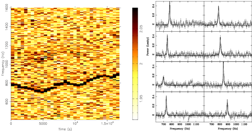
Figure 1.  : Left Panel: Dynamic power spectrum of the source 4U 1728–34. Right Panel: Power spectra of some selected intervals.

As I already mentioned, one property of the kHz QPOs is that their frequencies vary with time (therefore the underlying time series is non-stationary). This is shown in Figure 1, for the source 4U 1728–34. On the left panel I show a dynamical power spectrum, where the x-axis represents time (the origin of time in this case is 1997 October 1 at 06:09 UTC), the y-axis is the Fourier frequency, and the different gray levels indicate the power in each frequency bin. The dark feature that crosses the Figure almost horizontally is one of the two QPOs detected in this source. The right panel shows power spectra ($P(\nu)$ vs. Fourier frequency) at some selected times: The same QPO is seen moving between $\sim 700$ and 900 Hz.

Figure 2.  : Left Panel: Average (standard) power spectrum of the same data shown in Figure 1. Right Panel: Shifted-and-averaged power spectrum of the same data.

Obviously, the average power spectrum of the whole observation will show several peaks, at the frequencies at which the QPO stays for a while during the observation. This is shown in Figure 2 left panel, where the average power spectrum has been calculated as described above. However, as the QPO is strong enough to allow us to measure it in short time segments, we can think of “shifting” the frequency axis of each individual power spectrum before we calculate the average so that the new power spectrum is $\tilde{P}(\nu)=<X^{2}_{n}(\nu-\nu_{0,n})>$. Here $\nu_{0,n}$ is the frequency shift that we need to apply to the power spectrum of each segment if we want to align the strong QPO at the same frequency before we calculate the average. Notice that this is equivalent to multiplying the function $x(t)$ by $e^{-2\pi i\nu_{0,n}t}$ before calculating the integral in eq.(1).

The right panel in Figure 2 shows the result of such procedure (which, of course, also implies measuring $\nu_{0,n}$ for each segment; certainly this is extra work, but it comes with some rewards, as I will explain in §3). If it were only for the strong QPO in the average power spectrum (this QPO is stronger in the new power spectrum than in the original one) we would have not gained much by this procedure. Although there is now only one sharp peak, this shifted-and-averaged power spectrum provides no new information about the strong QPO. However, there is a second (weaker, but yet significant) QPO in the shifted power spectrum, $\sim 350$ Hz above the strong QPO. Although there seems to be evidence for such a weak QPO in the original power spectrum (Fig. 2, left panel), there it was not significant enough.

To understand why we detect this QPO in the shifted power spectrum, while in the standard power spectrum it was not significant enough, we need to recall that the $S/N$-ratio of the QPO is proportional to $(T/W)^{1/2}$, where $T=N\times\tau$ is the total length of the observation, and $W$ is the width of the QPO (see van der Klis 1989b). If the frequency separation between the 2 QPOs is roughly constant (a close inspection to Fig. 1 left panel shows that there might be such weak QPO in the dynamic power spectrum, “following” the strong QPO as this one moves in frequency), the shift applied to the power spectra of the individual segments to align the strong QPO also aligns the weak QPO. This makes this new QPO narrower, and therefore more significant, in $\tilde{P}(\nu)$ than in $P(\nu)$.

This is how we first discovered the second QPO during 1996 outburst of 4U 1608–52 (Méndez et al. 1998a), which we afterwards detected again (this time without requiring the sensitivity-enhancing technique described above) during another outburst in 1998 (Méndez et al. 1998b).

Not surprisingly, this same technique can be used to obtain much better measurements of the frequency separation between the kHz QPOs. This is because the error in the centroid frequency of a QPO is proportional to the width of the QPO, and inversely proportional to its S/N-ratio (see Downs & Reichley 1983 for a similar situation when measuring the arrival time of individual pulses in radio pulsars). As described above, the weak QPO is usually narrower in the shifted power spectrum, $\tilde{P}(\nu)$, than in the standard power spectrum, $P(\nu)$, and therefore its frequency can be measured more accurately in $\tilde{P}(\nu)$ than in $P(\nu)$.

One way of measuring $\Delta\nu$ using the shifted power spectrum is the following: Divide the data into $N$ segments of length $\tau$, and for each segment calculate the power spectrum. Measure the frequency of the strong QPO, $\nu_{1}$, in each of these $N$ power spectra, and group the data in $M$ sets such that $\nu_{1}$ is more or less constant within each set. This ensures that $\Delta\nu$ is more or less constant within each set (early results in Sco X–1 showed that $\Delta\nu$ decreased monotonically as $\nu_{1},\nu_{2}$ increased; van der Klis et al. 1997). For each set, align the power spectra of the individual time segments using $\nu_{1}$ as a reference, and combine them to produce an average power spectrum. The result is $M$ (aligned) power spectra for which both kHz QPOs are as narrow as possible. For each of these $M$ power spectra measure $\nu_{1}$ and $\nu_{2}$, calculate $\Delta\nu=\nu_{2}-\nu_{1}$, and plot $\Delta\nu$ vs. the average value of $\nu_{1}$ in each set.

Figure 3.  : Left Panel: Frequency separation between the two simultaneous kHz QPOs in 4U 1608–52 (circles) and Sco X–1 (crosses). Right Panel: Frequency separation between the two simultaneous kHz QPOs in 4U 1728–34 (circles). The solid line indicates the frequency of the burst oscillations at 363.95 Hz (Strohmayer et al. 1996). The dashed line indicates the average value of $\Delta\nu$ (349.3 Hz) for the first 6 points. For the three sources $\Delta\nu$ as a function of $\nu_{1}$ was calculated as explained in the text.

Figure 3 shows the results of applying such procedure to the kHz QPOs in 4U 1608–52, 4U 1728–34, and Sco X–1. The implications of these results (specially in the case of 4U 1728–34) to the existing models for the kHz QPOs are presented elsewhere in this book (see the chapter by van der Klis), and will not be discussed here.

3 Other Results

As I mentioned in §2, there is a reward for the extra work of measuring $\nu_{1}$ in the individual time segments: We can combine these measurements with, for instance, the source count rate or X-ray colors in those same segments. One example of this is shown in Figure 4. The left panel shows a plot of $\nu_{1}$ vs. the $2-16$ keV count rate for 4U 1608-52. Each point represents 128 s of data. For the same data used in the plot on the left panel, the right panel shows the relation between $\nu_{1}$ and an X-ray color (see the caption of this figure for the definition of the color).

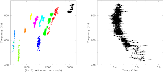
Figure 4.  : Left Panel: Relation between $\nu_{1}$ and the $2-16$ keV count rate in 4U 1608–52. Right Panel: For the same data as on the left panel, $\nu_{1}$ vs. X-ray hard color, defined as the ratio of the count rate in the $6.0-9.7$ keV band to the count rate in the $9.7-16.0$ keV band.

Interesting in this Figure is the complex dependence of $\nu_{1}$ upon X-ray count rate, which is usually assumed to be a good measure of mass accretion rate $\dot{M}$, and how this complexity is reduced to a single track in the frequency vs. hard color diagram. As before, the interested reader can find an extensive discussion of this subject elsewhere in this book. I just want to say here that these are “side” results of the technique described in §2.

4 Conclusion

I presented a new technique aimed at increasing the sensitivity to weak moving QPOs in the power density spectra of LMXBs. I showed some examples of the results obtained by applying this technique to data obtained with the Rossi X-ray Timing Explorer. In particular, this technique provides more precise measurements of the frequencies of the kHz QPOs, which can be used to set constraints on the models so far proposed to explain this new phenomenon.