For submission to Monthly Notices
Evolution of the probability distribution function of galaxies in redshift-space

Abstract

We present a new analytic calculation for the redshift-space evolution of the 1-point galaxy Probability Distribution Function (PDF). The nonlinear evolution of the matter density field is treated by second-order Eulerian perturbation theory and transformed to the galaxy density field via a second-order local biasing scheme. We then transform the galaxy density field to redshift space, again to second order. Our method uses an exact statistical treatment based on the Chapman–Kolmogorov equation to propagate the probability distribution of the initial mass field to the final redshifted galaxy density field. We derive the moment generating function of the PDF and use it to find a new, closed-form expression for the skewness of the redshifted galaxy distribution. We show that our formalism is general enough to allow a non-deterministic (or stochastic) biasing prescription. We demonstrate the dependence of the redshift space PDF on cosmological and biasing parameters. Our results are compared with existing models for the PDF in redshift space and with the results of biased N-body simulations. We find that our PDF accurately models the redshift space evolution and the nonlinear biasing.

1 Introduction

One of the central goals of modern cosmology is to gain a quantitative understanding of the nature of the observed galaxy distribution. In order that such an understanding be complete it must incorporate an explanation of both the evolution of large-scale structure in the universe and of the relationship between galaxies and the underlying dark mass.

In the standard paradigm the origin of structure can be traced back to small perturbations in the mass density imprinted during an inflationary phase. These perturbations subsequently grow in amplitude through gravitational instability. This prescription is well tested in N-body simulations and can be used to make useful predictions about the clustering history of dark matter. Many of the details, however, are not well understood.

The picture becomes more complex when one considers the galaxy distribution. Firstly, the astrophysical processes that govern the formation of the galaxies themselves introduce a nontrivial relationship between the galaxies and the dark matter. This relationship is generally termed galaxy bias. The biasing relation may prove to be simple to describe, depending only upon the local density in dark matter at a given point (eg Coles 1993). Conversely it could be extremely complex, depending on the larger scale environment, tidal fields, feedback and entire history of the galaxy formation site. This could lead to non-local (Bower et al. 1993) or non-deterministic forms of biasing (Pen 1998, Dekel & Lahav 1999). Secondly, the observed galaxy distribution is distorted in 3D redshift catalogues due to the line of sight components of the galaxy peculiar motions adding to the general Hubble expansion (Kaiser 1987). These redshift distortions, if not properly modeled, may lead to misinterpretation when comparing theory with observation.

A complete specification of galaxy clustering may only truly be given by the full set of galaxy N-point correlation functions. Such functions form the solution to the so-called BBGKY system of dynamical equations. This approach, pioneered in the 1970s by Peebles and co workers (Davis & Peebles 1977, Groth & Peebles 1977, Fry & Peebles 1978, Peebles 1980), has met with little success in practice. From a theoretical perspective, a closed solution to the BBGKY hierarchy has never been found and remains a thorny problem. Observationally, measurements of the correlation functions have been restricted to the lowest few orders.

An alternative description, and the focus of this work, may be given by the Probability Distribution Function (PDF) of a random field. Strictly, we investigate the PDF at a single spatial location (the 1-point PDF), but in general the PDFs are a family of N-point distribution functions for the probability at N positions in space. The random fields of interest are the density fields of both dark matter and galaxies.

PDFs are useful in cosmology because, in principle, they encode much of the information contained within the full hierarchy of correlation functions, thus providing valuable information about gravitational evolution and initial conditions. Furthermore the discrete analogy of the 1-point PDF, the counts in cells statistic, is a relatively straightforward quantity to measure from galaxy surveys (Hamilton 1985, Alimi et al. 1990, Szapudi et al. 1992, 1996, Gaztañaga 1992, 1994, Bouchet et al. 1993, Kim & Strauss 1998), allowing for easy comparison between theory and observation.

The shape of the PDF is strongly influenced by the non-linear effects of gravitational instability. A cosmic field that is initially Gaussian random, the generic prediction of most inflationary models, will remain so only when its evolution is linear. When the evolution becomes nonlinear, the higher-order moments of the field (more correctly the cumulants) become non-zero for the first time resulting in a PDF that may be strongly skewed about its mean and cuspy around its peak.

Attempts to describe theoretically this evolution have been numerous (Fry 1985, Coles & Jones 1991, Bernardeau 1992, 1994, 1996, Bernardeau & Kofman 1995, Juszkiewicz et al. 1995, Colombi et al. 1997, Gaztanaga et al. 1999, Taylor & Watts 2000) with the result that, at least for quasi-linear evolution of the matter field, the behavior of the PDF is quite well understood. Since the density field of galaxies inferred from a galaxy redshift survey may not be a good representation of the underlying dark matter it is unlikely that the PDF of the dark matter density field is a realistic approximation for that of galaxies. Just as nonlinear gravitational evolution drives the PDF away from Gaussianity, so too will nonlinear bias and redshift distortions. The challenge is to separate out each of the effects and quantify the evolution of the PDF in terms of a few essential parameters.

There have been significantly fewer attempts to calculate the evolution of the PDF in redshift space than in real space. Most notably, Hui et al. (2000) extended the work of Bernardeau & Kofman (1995) to calculate the evolution using the Zel’dovich approximation. Despite being an excellent approximation for the nonlinear gravitational dynamics Zel’dovich’s solution does not produce a good fit to the PDF of N-body simulations. This is principally due to the formation of caustics in the density field at shell crossing. The result for the Zel’dovich PDF is an asymptotic high density tail that falls off like $\delta^{-3}$ in both real and redshift space. Tails like these are not observed in simulations.

Another way of incorporating the effect of redshift distortions and bias is to use the Edgeworth expansion (Juszkiewicz et al. 1995, Bernardeau & Kofman 1995). In this approximation, the PDF is reconstructed from the moments of the field which must be calculated separately using perturbation theory. Such a calculation was done by Juszkiewicz et al. (1993; but see Hivon et al. 1995 for more details), who used second order Lagrangian perturbation theory (Bouchet et al. 1995) to map the skewness of an unbiased field into redshift space. They did not, however, try to use the skewness to evolve the PDF via the Edgeworth expansion.

A problem with using the Edgeworth expansion is its tendency to produce unphysical features in the PDF. In particular is the appearance of negative probabilities at low densities and the formation of unphysical “wiggles” in the high density tail of the distribution when the variance grows. These problems can be overcome by reconstructing the PDF using a Gamma expansion (Gaztañaga et al. 1999) which shows a markedly better agreement with N-body data in real space.

In this paper we extend the formalism developed in a earlier work (Taylor & Watts 2000, henceforth TW2000) where we showed how the PDF transforms when the matter density field is propagated to second-order. This method is based on an exact propagation of Gaussian initial probabilities using the Chapman–Kolmogorov equation from statistical physics (e.g van Kampen 1992). In this paper we develop this approach to include the transformation to a local, second-order biased galaxy distribution, and apply second-order Eulerian perturbation theory to describe the mapping into redshift-space. We show how the method can be naturally extended to incorporate a stochastic (or hidden variable) bias, although we leave detailed calculations for a later paper (Watts & Taylor in preparation). Our calculation also provides a new analytic solution for the skewness in redshift-space. This result is different to that of Hivon et al. (1995) who estimated the skewness by inverse transform of the bispectrum. However they where unable to find a closed-form solution, and did not include the effects of nonlinear galaxy biasing. Here we derive a closed-form solution for the skewness, including second-order bias, and find that the nonlinear bias has a large effect.

The layout of this paper is as follows. In §2 we discuss the derivation of the 1-point Probability Distribution Function. The new result for the skewness, and a discussion of stochastic biasing may also be found here. In §3 we illustrate the various dependencies on cosmological parameters of the shape of the PDF. Our results are compared with N-body simulations and other approximations in §4, conclusions are given in §5.

2 The galaxy distribution function in redshift-space

2.1 Redshift distortions and biasing in second-order perturbation theory.

2.1.1 Second-order perturbation theory

In Eulerian perturbation theory the density field $\delta(\mbox{\boldmath$x$},t)$ at real space comoving position $x$ and time $t$ in a flat Universe can be expanded into a series of separable functions;

$$\delta(\mbox{\boldmath$x$},t)=\sum_{n=1}^{\infty}\delta_{n}(\mbox{\boldmath$x$},t)=\sum_{n=1}^{\infty}D_{n}(t)\varepsilon_{n}(\mbox{\boldmath$x$}),$$ (1)

In curved space this expansion is only separable to second-order. The evolution of $\delta(\mbox{\boldmath$x$},t)$ can therefore be traced into the nonlinear regime by solving the fluid and Poisson’s equations for each order in the perturbation expansion (Peebles 1980, Juszkiewicz 1981, Vishniac 1983, Fry 1984, Bouchet et al. 1992, Bouchet et al. 1995);

$$\delta = \delta_{1}+\delta_{2}$$ (2)

$$= \delta_{1}+\frac{1}{3}(2-\kappa)\delta_{1}^{2}-\mbox{\boldmath$\eta$}.\mbox{\boldmath$g$}+\frac{1}{2}(1+\kappa)E^{2},$$

where

$$\mbox{\boldmath$\eta$}(\mbox{\boldmath$x$},t)=\mbox{\boldmath$\nabla$}\delta_{1}(\mbox{\boldmath$x$},t),$$ (3)

is the gradient of the linear density field and

$$\mbox{\boldmath$g$}(\mbox{\boldmath$x$},t)=-\mbox{\boldmath$\nabla$}\nabla^{-2}\delta_{1}(\mbox{\boldmath$x$},t),$$ (4)

is the linear peculiar gravity field where $\nabla^{-2}$ is the inverse Laplacian. The trace-free tidal tensor is given by

$$E_{ij}(\mbox{\boldmath$x$},t)=(\nabla_{i}\nabla_{j}\nabla^{-2}-\frac{1}{3}\delta_{ij})\,\delta_{1}(\mbox{\boldmath$x$},t).$$ (5)

2.1.2 Redshift space distortions

To determine the redshift space density field one must consider the mapping from the real space comoving position to redshift space comoving position, $s$, given by (see the excellent review by Hamilton, 1998, for a full account)

$$\mbox{\boldmath$s$}=\mbox{\boldmath$r$}+\hat{\mbox{\boldmath$r$}}u$$ (6)

where $u=\hat{\mbox{\boldmath$r$}}\cdot\mbox{\boldmath$v$}(\mbox{\boldmath$r$},t)/H_{0}$ is the projection of the velocity field along the line of sight. In the distant observer approximation (Kaiser 1987) the result can be written as a series in $u$ and $\delta$,

$$\delta^{s}(\mbox{\boldmath$s$},t)=\sum_{n=0}^{\infty}\frac{(-u)^{n}}{n!}\frac{\partial^{n}}{\partial s^{n}}\left(\frac{\delta(\mbox{\boldmath$s$},t)-u^{\prime}}{1+u^{\prime}}\right),$$ (7)

where ${}^{\prime}\equiv\partial/\partial r$ and all quantities are evaluated in redshift-space coordinates.

Expanding this to second order we find

$$\delta^{s}=\delta-u^{\prime}-[u(\delta-u^{\prime})]^{\prime}.$$ (8)

2.1.3 Galaxy bias

Next we assume that the density field of galaxies, smoothed on some scale $R$, is some local function of the underlying smoothed field of dark mass. Following Fry & Gaztañaga (1993) we expand the galaxy density in powers of $\delta$;

$$\delta_{g}=\sum_{n}\frac{b_{n}}{n!}\delta^{n}.$$ (9)

The coefficients in this expansion, $b_{n}$, are the bias parameters. We make no assumptions about the biasing function other than that it is local and that it may be expanded in a Taylor series. This is a deterministic Eulerian biasing scheme, but can be generalised to a stochastic Eulerian biasing scheme to allow for the hidden effects of galaxy formation (Pen 1998, Dekel & Lahav 1999). In Section 2.4 we show how our intrinsically probabilistic approach can be used to incorporate a stochastic Eularian bias. Other alternatives for bias are nonlocal Eulerian biases (Bower et al. 1993) and Lagrangian biasing schemes, which are intrinsically nonlocal in Eulerian coordinates. The latter is possibly the most natural to arise from following halos in the Press-Schechter approach to galaxy formation (Press & Schechter 1974). Our approach is more phenomenological and we do not consider these possibilities here.

Combining equations (7) and (9) gives to second order (Heavens et al. 1998)

$$\delta^{s}_{g}=b_{1}\delta-u^{\prime}+\frac{b_{2}}{2}(\delta^{2}-\sigma_{0}^{2})+u^{\prime 2}-b_{1}\delta u^{\prime}-b_{1}\delta^{\prime}u+uu^{\prime\prime}$$ (10)

where all quantities are evaluated at $s$.

In order that this expression has the correct expectation value, $\langle\delta_{g}^{s}\rangle=0$, we have set $b_{0}=-b_{2}\sigma_{0}^{2}/2$. Finally we rewrite equation (10) in terms of the linear density, gravity and tidal fields we shall use in later calculations;

$$\delta^{s}_{g}=\delta^{s}_{g,1}+\delta^{s}_{g,2}+\Delta^{s}_{g,1}+\Delta^{s}_{g,2},$$ (11)

where

$$\delta^{s}_{g,1}=b_{1}\delta_{1},$$ (12)

$$\delta^{s}_{g,2}=b_{1}\delta_{2}+\frac{b_{2}}{2}(\delta_{1}^{2}-\sigma_{0}^{2}),$$ (13)

$$\Delta^{s}_{g,1}=f_{1}\left(E_{zz}+\frac{\delta_{1}}{3}\right),$$ (14)

$$\Delta^{s}_{g,2} = \Delta^{s2}_{g,1}+\delta^{s}_{g,1}\Delta^{s}_{g,1}-\frac{f_{2}}{3}\kappa\left(\Pi_{zz}^{\delta}+\frac{\delta_{1}^{2}}{3}\right)$$ (15)

$$+ \frac{f_{2}}{2}\kappa\left(\Pi_{zz}^{E}+\frac{E^{2}}{3}\right)-f_{1}g_{z}\left(b_{1}\eta_{z}+f_{1}F_{zzz}\right).$$

The first two terms in equation (11) deal with the non-linear evolution and second order bias, the last two terms bring in the effects of redshift distortions.

The new dynamical variables required for redshift-space are the gradient of the tidal field

$$F_{ijk}(\mbox{\boldmath$r$},t)=\nabla_{i}\nabla_{j}\nabla_{k}\nabla^{-2}\delta_{1}(\mbox{\boldmath$r$},t),$$ (16)

and the second-order tidal fields

$$\Pi^{\delta}_{ij}(\mbox{\boldmath$r$},t)=(\nabla_{i}\nabla_{j}\nabla^{-2}-\frac{1}{3}\delta_{ij})\,\delta_{1}^{2}(\mbox{\boldmath$r$},t),$$ (17)

and

$$\Pi^{E}_{ij}(\mbox{\boldmath$r$},t)=(\nabla_{i}\nabla_{j}\nabla^{-2}-\frac{1}{3}\delta_{ij})\,E^{2}(\mbox{\boldmath$r$},t).$$ (18)

Note that in writing equations (11) to (15) we have made the plane parallel approximation, evaluating all of the redshift space contributions along a single cartesian axis.

The remaining parameters in the second-order model are (Bouchet et al. 1992, see also Catelan et al. 1995)

$$\kappa\equiv\frac{D_{2}}{D^{2}_{1}} \approx -3/7\Omega^{-2/63}\hskip 36.135pt{\rm open\,\,\,universe}$$ (19)

$$\approx -3/7\Omega_{m}^{-1/143}\hskip 32.52127pt{\rm flat\,\,\,universe}$$

where $\delta_{1}(\mbox{\boldmath$x$},t)=D_{1}(t)\varepsilon_{1}(\mbox{\boldmath$x$})$, and $D_{1}(t)\approx(1+z)^{-\Omega^{0.6}}$ is the linear growth function for an open model (Peebles 1980). The redshift-space parameters are (Peebles 1980, Lahav et al. 1991, Martel 1991)

$$f_{1}\equiv\frac{d\ln D_{1}}{d\ln a} \approx \Omega_{m}^{3/5}\hskip 28.90755pt{\rm open\,\,\,universe}$$ (20)

$$\approx \Omega_{m}^{5/9}\hskip 32.52127pt{\rm flat\,\,\,universe}$$

and (Hivon et al. 1995)

$$f_{2}\equiv\frac{d\ln D_{2}}{d\ln a} \approx 2\Omega^{4/7}\hskip 25.29494pt{\rm open\,\,\,universe}$$ (21)

$$\approx 2\Omega_{m}^{6/11}\hskip 21.68121pt{\rm flat\,\,\,universe}$$

Note that our expression for the redshift distorted and biased galaxy distribution, equation (11), does not agree with Hivon et al. (1995), even taking into account their slightly different projection into redshift space. Hivons et al.’s expression does not appear to have the correct expectation value, i.e. their quantity $\langle\delta^{s}\rangle\neq 0$.

2.2 The distribution of initial fields

Following the analysis of TW2000 we aim to find the joint probability for the fields in equation (10). Defining the parameter vector $\mbox{\boldmath$y$}=(\delta_{1},\mbox{\boldmath$\eta$},\mbox{\boldmath$g$},\mbox{\boldmath$E$},\Pi^{\delta}_{zz},\Pi^{E}_{zz},F_{zzz})$, the initial distribution function is given by

$$P(\mbox{\boldmath$y$})=\frac{1}{((2\pi)^{n}\mid\det{\mbox{\boldmath$C$}}\mid)^{1/2}}\exp{\left(-\frac{1}{2}\mbox{\boldmath$y$}^{t}\mbox{\boldmath$C$}^{-1}\mbox{\boldmath$y$}\right)},$$ (22)

where the covariance matrix is

$$\mbox{\boldmath$C$}=\langle\mbox{\boldmath$y$}\mbox{\boldmath$y$}^{t}\rangle.$$ (23)

Taking the plane-parallel approximation for redshift-space distortions represents a significant simplification since any dependence of $\delta^{s}_{g}$ on the off-diagonal parts of $\Pi^{\delta}_{ij}$, $\Pi^{E}_{ij}$ and $F_{ijk}$ is removed, reducing the size of the required covariance matrix from $34\times 34$ to $15\times 15$.

Equation (22) is an approximation. The variables $\Pi^{\delta}$ and $\Pi^{E}$ are not strictly Gaussian random fields as they are generated from the square of linear fields. However, our definition of these quantities as trace-free makes them uncorrelated with all of the other fields. If we then assume that their distribution is Gaussian, as we may expect them to be as a result of the Central Limit Theorem, they become statistically independent Gaussian fields. To test our Gaussian approximation of the distribution of the $\Pi$-fields we generated random Gaussian $\delta$-fields and calculated $\Pi^{\delta}_{zz}$. From this we estimated its distribution and found that a Gaussian with variance $\sigma^{2}(\Pi^{\delta}_{zz})=8\sigma_{0}^{4}/45$ (see equation 24) was indeed a good approximation. Later on, in Section 2.5, we shall see that these terms do not contribute to the skewness of the final distribution to lowest order. Hence the effects of this approximation will only be apparent in the higher moments and at higher order.

The non-zero elements of the covariance matrix are given by.

$$\langle\delta^{2}\rangle = \sigma^{2}_{0},\hskip 36.98866pt\langle\eta_{i}\eta_{j}\rangle=\frac{1}{3}\sigma^{2}_{1}\delta_{ij},$$

$$\langle g_{i}g_{j}\rangle = \frac{1}{3}\sigma^{2}_{-1}\delta_{ij},\hskip 14.22636pt\langle\eta_{i}g_{j}\rangle=\frac{1}{3}\sigma^{2}_{0}\delta_{ij},$$

$$\langle E_{ij}E_{kl}\rangle = \frac{1}{15}\sigma^{2}_{0}\left(\delta_{ik}\delta_{jl}+\delta_{il}\delta_{jk}-\frac{2}{3}\delta_{ij}\delta_{kl}\right)$$

$$\langle\Pi^{\delta}_{zz}\Pi^{\delta}_{zz}\rangle = \frac{8}{45}\sigma^{4}_{0}\hskip 17.07182pt\langle\Pi^{E}_{zz}\Pi^{E}_{zz}\rangle=\frac{22}{135}\sigma^{4}_{0}$$

$$\langle g_{i}F_{jkl}\rangle = \frac{1}{15}\sigma_{0}^{2}(\delta_{ij}\delta_{kl}+\delta_{ik}\delta_{jl}+\delta_{il}\delta_{jk})$$

$$\langle F_{zzz}\eta_{z}\rangle = \frac{1}{5}\sigma_{0}^{2}\hskip 22.76228pt\langle F_{zzz}F_{zzz}\rangle=\frac{1}{7}\sigma_{1}^{2}$$ (24)

Evaluating the action of equation (22) we find

$$\mbox{\boldmath$y$}^{t}\mbox{\boldmath$C$}^{-1}\mbox{\boldmath$y$} = \frac{\delta^{2}}{\sigma_{0}^{2}}+\frac{3}{(1-\gamma_{\nu}^{2})}\left(\frac{\eta^{2}}{\sigma_{1}^{2}}+\frac{g^{2}}{\sigma_{-1}^{2}}-2\gamma_{\nu}\frac{\mbox{\boldmath$\eta$}.\mbox{\boldmath$g$}}{\sigma_{1}\sigma_{-1}}\right)$$ (25)

$$+ 15\frac{E^{2}}{\sigma_{0}^{2}}+\frac{63}{4\sigma_{1}^{2}}\left(\eta_{z}-\frac{5}{3}F_{zzz}\right)^{2}$$

$$+ \frac{45}{8\sigma_{0}^{4}}\left(\Pi^{\delta}_{zz}\right)^{2}+\frac{135}{22\sigma_{0}^{4}}\left(\Pi^{E}_{zz}\right)^{2},$$

with determinant

$$\det{\mbox{\boldmath$C$}}=\frac{22}{7}\frac{2^{5}}{3^{15}5^{9}}\sigma_{0}^{32}\sigma_{1}^{2}\frac{(1-\gamma_{\nu}^{2})^{3}}{\gamma_{\nu}^{6}}.$$ (26)

The correlation parameter is defined by

$$\gamma_{\nu}\equiv\frac{\sigma_{0}^{2}}{\sigma_{1}\sigma_{-1}}.$$ (27)

which is the correlation coefficient of the velocity and gradient density fields. The variances are defined as

$$\sigma_{n}^{2}(k)=D_{1}^{2}(t)\int_{0}^{\infty}\!\frac{dk}{2\pi^{2}}\,k^{2+2n}P(k)e^{-k^{2}R_{s}^{2}},$$ (28)

where $R_{s}$ is the smoothing scale. For linear CDM power spectra $\gamma_{\nu}$ is found to lie in the range $0.50<\gamma_{\nu}<0.65$ (TW2000) for a wide range of scales. TW2000 discuss the effect of varying $\gamma_{\nu}$ and find that it is very small in the given range. We henceforth adopt the value $\gamma_{\nu}=0.55$ for all subsequent plots.

2.3 Propagation of the density distribution function

The multivariate Gaussian distribution for initial fields is propagated to later times using the Chapman-Kolmogorov equation;

$$P(\mbox{\boldmath$\beta$})=\int d\mbox{\boldmath$\alpha$}W(\mbox{\boldmath$\alpha$}|\mbox{\boldmath$\beta$})P(\mbox{\boldmath$\alpha$}).$$ (29)

where $W(\mbox{\boldmath$\alpha$}|\mbox{\boldmath$\beta$})$ is the transition probability from the state $\alpha$ to $\beta$. For a deterministic process, such as the gravitational evolution of a system from the linear to non-linear regimes, the transition probability is given by a Dirac delta function

$$W(\delta^{s}_{g}|\mbox{\boldmath$y$})=\delta_{D}\left[\delta^{s}_{g}-\delta^{s}_{1}-\delta^{s}_{2}-\Delta^{s}_{1}-\Delta^{s}_{2}\right].$$ (30)

The advantage of using the Chapman-Kolmogorov approach is that is generalizes the change of variables to allow for stochasticity in the transformation between initial and final states. This will be further discussed in §2.4.

The probability distribution function for $\delta^{s}_{g}$ can be written as an expectation over the stochastic variables $y$

$$P(\delta^{s}_{g})=\left\langle\delta_{D}(\delta^{s}_{g}-\delta^{s}_{1}-\delta^{s}_{2}-\Delta^{s}_{1}-\Delta^{s}_{2})\right\rangle_{y}$$ (31)

The Characteristic Function for $P(\delta^{s}_{g})$, defined by

$${\mathcal{G}}(J)\equiv\int_{-\infty}^{\infty}d\delta^{s}_{g}P(\delta^{s}_{g})\exp\left(-iJ\delta^{s}_{g}\right)$$ (32)

and with inverse

$$P(\delta_{g}^{s})=\int_{-\infty}^{\infty}\!\frac{dJ}{2\pi}\,{\mathcal{G}}(J)\exp\left(iJ\delta^{s}_{g}\right)$$ (33)

can be expressed as the expectation value

$${\mathcal{G}}(J)=\left\langle\exp{-iJ(\delta^{s}_{1}+\delta^{s}_{2}+\Delta^{s}_{1}+\Delta^{s}_{2})}\right\rangle_{y}.$$ (34)

As in TW2000, equation (34) reduces to a set of Gaussian type integrals which yield the probability generating function, ${\mathcal{G}}(J)$, for a smoothed galaxy density field in redshift space;

$${\mathcal{G}}(J) = \prod_{i=1}^{5}\theta_{i}^{-1/2}\exp{\left[-\frac{1}{2}iJ\sigma_{0}^{2}b_{2}\right]}\exp{\left[-\frac{J^{2}\sigma_{0}^{2}N^{2}}{2\theta_{1}}\right]}$$ (35)

$$\times \exp{\left[-\frac{2}{45}\frac{J^{2}\sigma_{0}^{2}f_{1}^{2}}{\theta_{3}}\left(1-\frac{iJ\sigma_{0}^{2}NH}{f\theta_{1}}\right)^{2}\right]}$$

$$\times \exp{\left[-\frac{1}{2}J^{2}\sigma_{0}^{8}f_{2}^{2}\kappa^{2}\frac{1379}{1080}\right]}$$

where

$$\theta_{1} = 1+2iJ\sigma_{0}^{2}A$$

$$\theta_{2} = \left(1+\frac{4}{15}iJ\sigma_{0}^{2}B\right)^{4}$$

$$\theta_{3} = 1+\frac{4}{15}iJ\sigma_{0}^{2}B+\frac{8}{45}iJ\sigma_{0}^{2}f_{1}^{2}+\frac{8}{45}\frac{J^{2}\sigma_{0}^{4}H^{2}}{2\theta_{1}}$$

$$\theta_{4} = \left(1-\frac{2}{3}iJ\sigma_{0}^{2}b_{1}+\frac{1}{9}J^{2}\sigma_{0}^{4}b_{1}^{2}\frac{(1-\gamma_{\nu}^{2})}{\gamma_{\nu}^{2}}\right)^{2}$$

$$\theta_{5} = 1-i\frac{1}{5}J\sigma_{0}^{2}\left(f_{1}^{2}-\frac{10}{3}M\right)$$

$$+ J^{2}\sigma_{0}^{4}\left[M\frac{(1-\gamma_{\nu}^{2})}{9\gamma_{\nu}^{2}}\left(M+\frac{18}{15}f_{1}^{2}\right)+\frac{1}{21}\frac{f_{1}^{4}}{\gamma_{\nu}^{2}}\left(1-\frac{21}{25}\gamma_{\nu}^{2}\right)\right]$$

and

$$A = \frac{1}{3}(2-\kappa)b_{1}++\frac{1}{9}f_{1}^{2}+\frac{1}{3}b_{1}f_{1}-\frac{1}{9}f_{2}\kappa+\frac{1}{2}b_{2}$$

$$B = \frac{1}{2}(1+\kappa)b_{1}+\frac{1}{6}f_{2}\kappa$$

$$H = f_{1}\left(b_{1}+\frac{2}{3}f_{1}\right)$$

$$M = b_{1}(1+f_{1})$$

$$N = b_{1}+\frac{1}{3}f_{1}$$ (37)

The 1-pt PDF can then be found by numerical integration of equation (33). Equations (35) to (37) represent the main analytical result of the this paper.

2.4 Stochastic Bias Schemes

Instead of the local deterministic prescription for galaxy biasing described by equation (9) we may choose to implement a stochastic Eularian biasing scheme. In stochastic biasing (Pen 1998, Dekel & Lahav 1999) the relation between the underlying density field of dark matter and the galaxy density field is a random process with joint distribution $P(\delta_{g},\delta)$.

If we assume that the biasing transition distribution, $P(\delta_{g},\delta)$, is a bivariate Gaussian of the form

$$P(\delta_{g},\delta) = \frac{1}{2\pi[\sigma_{b}^{2}+b_{1}^{2}\sigma_{0}^{2}(1-r^{2})]}$$ (38)

$$\times \exp-\frac{1}{2}\frac{\delta_{g}^{2}+\delta^{2}b_{1}^{2}(1+\sigma_{b}^{2}/b_{1}^{2}\sigma^{2}_{0})-2rb_{1}\delta_{g}\delta}{\sigma_{b}^{2}+b_{1}^{2}\sigma_{0}^{2}(1-r^{2})},$$

where the covariances between the fields are given to first order by

$$\langle\delta_{g}^{2}\rangle = b_{1}^{2}\sigma_{0}^{2}+\sigma^{2}_{b},$$ (39)

$$\langle\delta_{g}\delta\rangle = b_{1}r\sigma_{0}^{2}$$ (40)

where $\sigma_{b}$ is the variance of the random component determining galaxy formation and $r$ is the correlation coefficient between the mass and galaxy distribution, then the galaxy distribution function can be written

$$P(\delta_{g})=\langle P(\delta_{g},f(\mbox{\boldmath$y$}))\rangle_{y},$$ (41)

where $f(\mbox{\boldmath$y$})=\delta_{1}+\delta_{2}$ in real space. The characteristic function for galaxies is then

$$G_{\delta_{g}}(J)=\int dJ^{\prime}G_{\delta}(J^{\prime})G_{\delta_{g},\delta}(J,J^{\prime})$$ (42)

where

$$\ln G_{\delta_{g},\delta}(J,J^{\prime})=-\frac{1}{2}(J^{2}\sigma_{0}^{2}+J^{\prime 2}(b_{1}^{2}\sigma_{0}^{2}+\sigma_{b}^{2})+2JJ^{\prime}b_{1}r\sigma_{0}^{2})$$ (43)

Equation (42) can be evaluated numerically.

The distribution function of galaxies can also be evaluated by numerically integrating

$$P(\delta_{g})=\int_{-\infty}^{\infty}\frac{dJ}{2\pi}{\mathcal{G}}_{\delta}(J)P(\delta_{g},J)$$ (44)

where

$$P(\delta_{g},J)=\int d\delta e^{iJ\delta}P(\delta_{g},\delta)$$ (45)

is the partially transformed characteristic function. We shall explore the effects of stochastic bias elsewhere, but note that it can be naturally incorporated into our probabilistic scheme. For the remainder of the paper we shall only discuss the deterministic scheme.

2.5 Skewness of a biased density field in redshift space

The skewness of the biased redshift-space galaxy distribution can be found from the characteristic function, ${\mathcal{G}}(J)$, by differentiation. The moment parameters are defined as

$$S_{n}=\frac{\langle\delta^{n}\rangle_{c}}{\sigma_{0}^{2n-2}},$$ (46)

where the cumulants (or connected moments) of the field are given by

$$\langle\delta^{n}\rangle_{c}=\frac{\partial^{n}}{\partial[iJ^{n}]}\ln{\mathcal{G}}(J=0).$$ (47)

In redshift space the skewness parameter becomes

$$S^{s}_{3}=\frac{\langle(\delta^{s}_{g})^{3}\rangle_{c}}{\sigma_{s}^{4}},$$ (48)

where $\sigma_{s}^{2}$ is the linear, redshift space variance of the galaxy density field, $\delta^{s}_{g}$.

Taking the third derivative and setting $J=0$ we find the redshift-space skewness parameter;

$$S^{s}_{3}b_{1}^{4}F^{2} = 4b_{1}^{3}\left(1+\frac{2}{3}\beta_{1}+\frac{3}{25}\beta_{1}^{2}\right)+3b_{2}b_{1}^{2}\left(1+\frac{\beta_{1}}{3}\right)^{2}$$ (49)

$$- 2\kappa b_{1}^{3}(1+\frac{1}{3}\beta_{2})\left(1+\frac{2}{3}\beta_{1}+\frac{7}{75}\beta_{1}^{2}\right)$$

$$+ 2b_{1}^{4}\beta_{1}\left(1+\frac{19}{15}\beta_{1}+\frac{3}{5}\beta_{1}^{2}\right)+\frac{6}{25}b_{1}^{4}\beta_{1}^{4}$$

where $F(\beta_{1})$ is the linear redshift space enhancement factor for the redshifted variance given to lowest order by (Kaiser 1987)

$$F=1+\frac{2}{3}\beta_{1}+\frac{1}{5}\beta_{1}^{2}.$$ (50)

and

$$\beta_{1}\equiv\frac{f_{1}}{b_{1}},\hskip 21.68121pt\beta_{2}\equiv\frac{f_{2}}{b_{1}}.$$ (51)

The variance in redshift space is just

$$\sigma_{s}^{2}=b_{1}^{2}\left(1+\frac{2}{3}\beta_{1}+\frac{1}{5}\beta_{1}^{2}\right)\sigma_{0}^{2}.$$ (52)

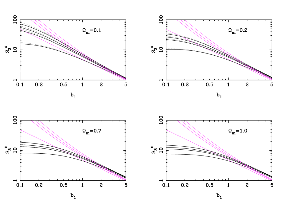
Figure 1: Log-log plot of the redshift-space galaxy skewness parameter, $S^{s}_{3}$, as a function of $\Omega_{m}$, $b_{1}$ and $b_{2}$. The panels show increasing values of $\Omega_{m}=0.1$, $0.2$, $0.7$, $1.0$. The x-axis is the linear bias parameter, $b_{1}$. Lines going up are the quadratic bias parameter $b_{2}=0.0$, $0.5$, $0.7$, $1.0$. Straight faint lines are the real space skewness, $S_{3}$, and are independent of $\Omega_{m}$. Darker curves are for the full redshifted skewness for an open (solid) and flat (dotted) universe.

Equation (49) for the galaxy skewness in redshift space is the second major result of this paper. It is interesting to compare this with the results of Hivon et al. (1995) who derived the density skewness in redshift space. Hivon et al. derived their result by transforming the redshifted bispectrum but did not find a closed form solution and were left with a term containing an integral that was to be determined numerically. Our result for the skewness should coincide with that of Hivon et al. for the special case of $b_{1}=1$ and $b_{2}=0$, but does not. The differences between our result and that of Hivon et al. may result from the different approaches, or from the difference in initial expressions for $\delta_{g}^{s}$. We have not not been able to trace the origin of these differences. We have verified equation (49) by a direct calculation of the redshifted galaxy skewness, using equation (11) along with the correlators in equation (24), to evaluate the quantity $\langle(\delta_{g}^{s})^{3}\rangle$.

Equation (49) displays the hierarchical scaling associated with galaxy clustering. It has already been shown that a local bias will retain a hierarchical form if the underlying field displays hierarchical behavior (Fry & Gastañaga 1993), and that the lowest order of perturbation theory reproduces the hierarchical structure. Our result would seem to indicate that this structure holds for galaxies in redshift-space. This is an important result as it strengthens the claim that if galaxies display a hierarchical scaling then it is consistent that the underlying density field was initially Gaussian distributed and bias is local. Our results suggest that this can be extended as a test of galaxy distributions in redshift-space.

In Figure 1 we plot the skewness parameter $S^{s}_{3}$ as a function of linear bias, $b_{1}$, for different values of $\Omega_{m}$ and a quadratic bias $b_{2}$. An immediate result is that in all the models the redshift-space skewness parameter, $S^{s}_{3}$, is less than the real-space skewness parameter, $S_{3}$, until $b_{1}>1.5$. This may seem surprising as one expects the effects of redshift space distortions will tend to make the density field look more evolved along the line of sight. This does happen, but the second-order skewness is dominated by the first-order increase in the variance, so that the ratio $\langle(\delta^{s})^{3}\rangle/\langle(\delta^{s})^{2}\rangle^{2}$ is smaller than its real space counterpart. This effect was previously observed by Hoyle et al. (2000).

Beyond $b_{1}\approx 1.5$ the redshift skewness parameter rises above its real space value for all the models. This is because for large values of the linear bias parameter the second order skewness becomes comparable in magnitude to the redshifted variance.

For $\beta_{1}\approx\beta_{2}\approx 1$ and $b_{1}\approx 1$ the redshifted skewness can be approximated by

$$S_{3}^{s}=\frac{1539}{343}b_{1}^{-0.61}\beta_{1}^{-0.02}+\frac{75}{49}\frac{b_{2}}{b_{1}^{2}}\beta_{1}^{-9/14}$$ (53)

which is accurate to a few percent. This can be compared with the undistorted skewness (Fry & Gaztañaga 1993)

$$S_{3}=\frac{34}{7}\frac{1}{b_{1}}+3\frac{b_{2}}{b_{1}^{2}}.$$ (54)

Without second-order bias, $S_{3}^{s}$ is only weakly dependent on $\beta_{1}$. The main effect of redshift-space distortions in this case is to change the dependence on $b_{1}$. The second-order bias term, however, has a much stronger dependence on $\beta_{1}$, and has a lower amplitude than the undistorted term when $\beta_{1}=1$.

Figure 2: The effect of linear and quadratic bias parameters on the 1-point PDF when the variance of the underlying mass density is $\sigma_{0}=0.2$. From left to right the linear bias is $b_{1}=$ 0.7, 1.0, 1.2. On the top row the second order bias parameter, $b_{2}$ is 0.0 and on the bottom 1.0. In all plots a solid line represents the PDF in real space, a dashed line is for redshift space when $\Omega=$ 0.3, and a dotted line for redshift space when $\Omega=$ 1.0.

3 The shape of the PDF

The solution for the generating function, ${\mathcal{G}}(J)$, given by equations (35) – (37) may be integrated numerically without too much difficulty to yield the full distribution function $P(\delta)$. In figure 2 we show the shape of the resulting PDF for a range of values of the parameters $b_{1},b_{2}$ and $\Omega_{m}$.

To second order there are two important quantities working to distort the shape of the PDF from a Gaussian with linear mass variance $\sigma_{0}$. Firstly is the variance of the resulting field which acts to broaden the distribution. Secondly is skewness, which produces asymmetry in the PDF about its mean at $\delta=0$. These two quantities are effected to varying degrees by non-linear evolution, by non-linear bias and by the distorting effect of galaxy peculiar motions.

For the plots in figure 2 we chose a moderate value for the linear variance of the underlying dark matter density field, $\sigma_{0}=0.20$. The correlation parameter, $\gamma_{\nu}$, was 0.55. In the top panel we show the effect of a purely linear bias with values $b_{1}=$0.7, 1.0 and 1.2 and with $b_{2}=0$. For the lower panel the linear $b_{1}$’s match those above but in this case $b_{2}=1.0$ for every plot. Each plot shows three different PDFs: one (solid lines) in real space, one in redshift space for the case $\Omega_{0}=1.0$ (dotted lines) and a third in redshift space but with $\Omega_{0}=0.3$ (dashed lines). We have inset the same plots on logarithmic axis in order to emphasize the tails of the distribution.

In real space and with linear bias only, the shape of the PDF is dominated by the $b_{1}^{2}$ boost to the variance. Where $b_{1}>1$ the change to $S^{s}_{3}$ is small and any effect on the shape of the PDF caused by the skewness is masked by the enhanced variance When $b_{1}<1$ there is a more substantial change to $S^{s}_{3}$ but in this case the variance becomes small enough that the PDF looks relatively Gaussian regardless of what is happening to the skewness.

To second order the non-linear bias parameter, $b_{2}$, does not alter the variance of the underlying mass density field. The changes to the shape of the PDF when $b_{2}\neq 0$ then reflect only the corresponding changes to $S^{s}_{3}$ We observe that the real space PDFs appear to peak sharply around $\delta=-1\sigma_{s}$ with an abrupt drop off of the low density tail to the left of the peak. The high density tail is extended beyond the corresponding case where $b_{2}=0$. With low $b_{1}$ the effect of $b_{2}$ is most pronounced, causing an increasingly abrupt drop off in $P(\delta)$ on the low density side of the peak. This pronounced effect on the PDF would appear to be an important signature of quadratic bias, which cannot be reproduced by any combination of other parameters.

Figure 3: Comparison with N-body simulation in real space when $\sigma_{s}=0.20$ and with linear bias $b_{1}=0.7$ (top panel) and $b_{1}=1.5$ (bottom panel). The solid line is the PDF for this work, the dotted line shows the reconstruction of the PDF from the Edgeworth expansion with the skewness parameter from §2. Filled squares represent the simulation data. The linear mass variance was $\sigma_{0}=0.29$ and 0.13 for the top and bottom plots respectively.

In redshift space the PDF is dominated by the enhancement of the variance due to linear redshift space distortions. As discussed in §2.5 the second-order change in the skewness is less than the linear change in variance resulting in a lower skewness parameter, $S_{3}^{s}$, in redshift-space than in real space. The result for the PDFs is a broader and less asymmetric appearance. This is most clearly seen in the PDFs where $b_{2}\neq 0$. For these plots, the sharp peak in $P(\delta)$ around $\delta=-1\sigma_{s}$ is significantly damped, and both the low and high density tails are much shallower than their real space counterparts.

4 Comparison of results with n-body simulations

4.1 The simulations

In this section we illustrate how our theoretical PDF compares with that measured from cosmological N-body simulations. For the comparison we chose to use Hugh Couchman’s Adaptive P³M N-body code (Couchman 1991) to model the evolution of the dark matter. The simulation volume was a cube of comoving side 200 $h^{-1}$Mpc with periodic boundary conditions. We chose a CDM initial power spectrum (Bardeen at al. 1986) that was normalized to match the present day abundance of clusters. The variance on a scale of 8 $h^{-1}$Mpc when the particle distribution was smoothed with top hat filters was $\sigma_{8}=0.5\ \Omega_{m}^{-0.5}$ in the final time-step of the simulation. The shape parameter used was $\Gamma=0.25$, representing the best fit of the CDM power spectrum to galaxy clustering data. The simulation was performed on a 128³ Fourier mesh with $100^{3}$ particles.

Figure 4: Comparison with N-body simulation in real space when $\sigma_{s}=0.20$ and with linear bias and second order bias. In the top panel $b_{1}=0.7$ while in the lower panel $b_{1}=1.0$ In both cases the second order bias parameter $b_{2}=1.0$. The solid line is the PDF for this work, the dotted line shows the reconstruction of the PDF from the Edgeworth expansion with the skewness from §2. Filled squares represent the simulation data. The linear mass variance was $\sigma_{0}=0.29$ and 0.13 for the top and bottom plots respectively.

We investigated the numerical PDFs in three sets of circumstances:

• in real space with bias,

• in redshift space without bias,

• in redshift space with bias.

The first two scenarios were trivial to construct from the simulations. For the case of bias in real space, we binned the data and estimated the overdensity from $\delta=(n_{p}-\bar{n}_{p})/\bar{n}_{p}$, where $n_{p}$ is the number of particles in a cell and $\bar{n}_{p}$ is the mean number of particles per cell. The biased distribution was then estimated by the transformation

$$\delta_{g}=b_{1}\delta+\frac{b_{2}}{2}(\delta^{2}-\sigma^{2}_{0})$$ (55)

where $\sigma_{0}$ is the variance on the scale of the binning.

Redshift distortions, in the absence of bias, were calculated using the peculiar velocities of the simulation particles. The distortions were made plane parallel in order to match our approximation from §2.1. The resulting particle distribution was smoothed with Gaussian filters of radius $R_{s}$. The PDF was then evaluated from the relative abundance of $\delta$ across the grid.

Measuring the combined effect of redshift distortions and bias was more difficult. A simple combination of the above methods could not be used, as we needed to identify biased galaxies before making the transformation to redshift space. Our basic biasing method calculates the biased density field on the grid so that information about individual galaxies was lost. In order to identify individual biased galaxies in the simulation we sampled a population of galaxies from the simulation particles so that the number of galaxies in a cell, $n_{g}$, was

$$n_{g}=\bar{n}_{g}\left[1+b_{1}\delta+\frac{b_{2}}{2}(\delta^{2}-\sigma_{0}^{2})\right].$$ (56)

The resulting distribution could then be transformed to redshift-space by using the galaxies velocity.

Figure 5: Comparison with N-body simulations in redshift space for $\Omega_{0}=1.0$ and $\Omega_{0}=0.3$ when $\sigma_{s}=0.2$. The bias parameters were in both cases $b_{1}=1.0$ and $b_{2}=0$, i.e no bias. The solid line is the PDF for this work, the dotted line shows the reconstruction of the PDF from the Edgeworth expansion with the skewness parameter from §2. Filled squared represents the simulation data. The linear mass variance was $\sigma_{0}=0.15$ and 0.17 for the top and bottom plots respectively.

The size of the grid was dictated by the need for $n_{p}$ to be sufficiently larger than $n_{g}$ so that underdense regions could be enlarged by the bias. Given this constraint we chose to smooth the particle distribution on a coarse mesh of between 9 and 11 cells, with a cell size of $l=22\,h^{-1}{\rm Mpc}$ and $18\,h^{-1}{\rm Mpc}$, respectively. As we calculate the linear variance using a Gaussian filter (equation 28) this corresponds to a smoothing scale of $Rs=l/\sqrt{12}=6.5$ and $5\,h^{-1}{\rm Mpc}$. The total number of galaxies was constrained by the requirement that $n_{g}$ was not larger than $n_{p}$ in areas of high density, so we set the total number in the simulation volume $N_{g}=5\times 10^{5}$.

The errors on the numerical PDFs for the biased and distorted only simulations were taken from the standard deviation over 5 independent realisations of the simulated volume. Errors due to shot noise were incorporated into the theoretical PDF (TW2000) based on the mean density of particles in a cubical cell of side $l=\sqrt{12}R_{s}$. In practice the shot noise contribution was small for simulations due to the high particle density.

In the case of a combined biased and redshift-space distorted PDFs the need to sample the galaxies on a coarser mesh meant that the resulting PDF from an individual simulation had a larger scatter from simulation to simulation for the same value of $\sigma_{s}^{2}$. To avoid this we used a simulation with a smaller clustering variance. A relatively large number of particles could then to be found in each cell. For the case $R_{s}\approx 5h^{-1}$Mpc there numbered on average 375 galaxies per cell sampled from around 750 simulation particles. When the numerical PDFs were averaged over 7 independent realisations the results were reasonably smooth, though the error bars (again the standard deviation over the 7 realisations) do reflect the scatter.

Figure 6: Comparison with N-body simulations showing the combined effect of bias and redshift distortions for $\Omega_{0}=1.0$ and when $\sigma_{s}=0.25$. The bias parameters were $b_{1}=1.2$ and $b_{2}=0$ in the upper panel and $b_{1}=1.0$, $b_{2}=1.0$ in the lower. The solid line is the PDF for this work, the dotted line shows the reconstruction of the PDF from the Edgeworth expansion with the skewness parameter from §2. Filled squared represents the simulation data. The linear mass variance was $\sigma_{0}=0.16$ and 0.19 for the top and bottom plots respectively.

4.2 The Edgeworth Expansion

In addition to the PDF calculated from this work we also examine the PDF reconstructed from the Edgeworth expansion (Juszkiewicz et al. 1995, Bernardeau & Kofman 1995) using the redshift-space skewness parameter derived in Section 2.5. The distribution function from the Edgeworth expansion is, to second order,

$$P(\nu)=\frac{1}{\sqrt{2\pi}}\left[1+\frac{1}{3!}H_{3}(\nu)S^{s}_{3}\right]\exp{\left[-\frac{1}{2}\nu^{2}\right]}$$ (57)

where $\sigma_{s}^{2}$ is the redshift-space galaxy variance given by equation (52), $S^{s}_{3}$ is the skewness parameter from equation (49), $H_{n}(\nu)$ is an $n^{th}$-order Hermite polynomial and $\nu=\delta^{s}/\sigma_{s}$ is the scaled redshift-space density field.

The main difference between the Edgeworth expansion and our own model for the PDF is that the Edgeworth relies upon two levels of approximation: firstly in the moments, which come from — in our case — a second order perturbative calculation; and secondly in the Edgeworth series itself, which reconstructs the non-linear PDF by expanding about a Gaussian distribution. Our PDF comes directly from the perturbation theory without any further constraints other than those implicit in the theory itself. In this way our model is perhaps more representative of the perturbation theory and its predictions and limitations. Another dissimilarity between the models, and a problem with trying to derive the PDF to second order, lies in the fact that second order perturbation theory does not get the higher moments of the distribution correct. In our calculation all of the higher moments exist but have terms missing that would come in in a higher order calculation. This may strongly effect the shape of our PDF, particularly around the peak. Such problems are not an issue for the Edgeworth and other similar approximations because in these models the cumulants are either put into the series explicitly, or else are zero.

4.3 Results

In comparing the models with simulation data we constructed the PDF so that the variance of the distorted, biased density field, $\sigma_{s}^{2}$, was constant for all choices of the parameters $\Omega$, $b_{1}$ and $b_{2}$. This was arranged by using an appropriate value for $\sigma_{0}$ for each plot. For the case of bias in real space and of no bias in redshift space we chose $\sigma_{s}=0.2$. This relatively moderate variance was necessary because for the cases where $b_{1}<1$ the underlying $\sigma_{0}$ had to start quite large. For the combination of bias and redshift distortions we were limited to starting with a slightly higher linear mass variance because the simulation PDFs became dominated by sampling variance when the cell size was large. For these plots $\sigma_{s}=0.25$.

Figures 3 and 4 show the behavior of the PDF with various combinations of the bias parameters and with no redshift space distortions. The density parameter for these simulations was $\Omega=1.0$, though in real space the quasi-linear evolution is not sensitive to this quantity (Bouchet et al. 1992, Martel & Freudling 1991).

The first set of plots (figure 3) show the effect of a linear bias only, $b_{1}=0.7$ in the top panel and $b_{1}=1.5$ in the bottom. The linear mass variance was $\sigma_{0}=0.29$ and $0.13$ respectively. The dominant effect on the shape is through the variance which tends to broaden and lower the amplitude PDF for $b_{1}>1$ and conversely makes the PDF more Gaussian when $b_{1}.<1$. The fit to the data (points) of the PDF from this work is good in both cases, though when $\sigma_{0}$ is relatively large our model misses the peak of the distribution and appears to be slightly too strongly skewed. The Edgeworth approximation (dotted lines) also shows excellent agreement with the simulations, particularly in the vicinity of the peak. The plots show the absolute value of the Edgeworth PDF. The “lobes” in the low density tail of the distribution represent negative probabilities in the Edgeworth PDF.

In figure 4 we show the fit to simulations when the second order bias term, $b_{2}$, is 1.0. The linear bias was set to $b_{1}=0.7$ (top) and $b_{1}=1.0$ (bottom). The linear mass variance was $\sigma_{0}=0.29$ (top) and $\sigma_{0}=0.20$ (bottom). To the order we are interested in $b_{2}$ only contributes to the PDF via $S_{3}$ and the higher moments. The effect of the second order bias is to fill in the void regions and enhance the peaks. The result for the PDF is a sharp drop-off of the low density tail and a dramatic amplification of the peak just beyond that point. The high density tail is also extended to account for the increased regions of very high density. The fit to the simulations for second order biasing is good so long as $\sigma_{0}$ is reasonably small, though still in the quasi-linear regime. The breakdown in the fit comes mainly in the low density tail which for the theoretical curves drops away too slowly when the variance is high. The Edgeworth PDF breaks down quite badly in the tails when $b_{2}\neq 0$. This suggests that the Edgeworth approximation becomes rather unstable when the skewness parameter is large, even when the variance is low. The peak of the Edgeworth PDF is not so badly affected, however, and fits the data nicely so long as $\sigma_{0}$ is not too high.

Figure 5 shows the fit of the PDF to an unbiased field of galaxies in redshift space. We ran two sets of simulations with $\Omega_{0}=$ 1.0 and 0.3. The linear variance used for the theoretical PDFs was $\sigma_{0}=0.15$ and $0.17$. The fit to both our model and the Edgeworth PDF is very good, although the linear variance in each case was quite small to ensure that $\sigma_{s}=0.2$. We found that our approximation began to break down when the redshift space variance was $\sigma_{s}=0.4$. Although the Edgeworth followed the peak and low density part of the distribution well to this variance and higher, its high density tail became unstable at a much lower $\sigma_{s}$. In both cases the PDFs look more Gaussian than in real space because of the reduction in $S^{s}_{3}$. The theoretical plots are almost identical in each case, as expected since we have arranged for the variance of the redshifted field to be identical in each case and anyway the skewness in redshift space is only very weakly dependant upon $\Omega_{m}$ when $b_{1}$ is close to unity. The numerical PDFs are marginally different, although we suspect that this is a numerical effect as suggested by the large error bars around the peak of the distribution for $\Omega_{m}=0.3$.

On much smaller scales we would expect there to be a real difference between the two PDFs as fingers of god, due to the pairwise velocities in clusters, become important. Our second-order analysis does not allow for these strongly nonlinear effects, and we restrict our analysis to scales large enough that these effects are not important. The agreement between theory and the simulations suggests that this is true. The effect we would expect to see would be a decrease in the variance and skewness of the PDFs in redshift-space.

Our final plots (figure 6) show the combined effect of both bias and redshift distortions. In the top row $b_{1}=1.2$ with $b_{2}=0.0$ and on the bottom we have set $b_{1}=1.0$ and made $b_{2}=1.0$. For both cases the density parameter was $\Omega_{m}=1.0$. In each of the plots $\sigma_{s}=0.25$ — due to problems with creating the bias/redshift simulations we were unable to satisfactorily measure the PDFs for $\sigma_{s}=0.2$. The linear mass variance was therefore $\sigma_{0}=0.18$ in the top plot and $0.19$ in the bottom. The fit in both cases is very good — although the Edgeworth approximation becomes slightly unstable when $b_{2}=1.0$ because of the relatively high skewness. Although the redshift distortions do wash out some of the effect of the bias parameters, there are dependencies which are reproduced by the models to a reasonable degree of accuracy. This is encouraging for the purposes of constraining cosmological models using the PDF and data from galaxy redshift surveys.

In general there is a good similarity between all of the numerical PDFs and those found from either our analysis based on the Chapman–Kolmogorov equation or the Edgeworth approximation with the redshift space skewness parameter $S^{s}_{3}$. The Edgeworth expansion clearly breaks down sooner in the tails of the distribution, and for large values of the skewness parameter. Considering that both models use second order perturbation theory and have the same skewness and variance it is perhaps confusing that they behave so differently with various combinations of the parameters. However we must not forget that the Edgeworth approximation and our model rely on very different approaches to obtain the PDF as discussed in §4.2.

Figure 7: Theoretical PDFs for a biased galaxy field in redshift space. The parameters are such that the combination $\beta=0.5$. For the solid curve $\Omega_{0}=1.0$ with $b_{1}=2.0$ and $b_{2}=0$ whereas for the dotted curve $\Omega_{0}=0.3$ with $b_{1}=1.0$ and $b_{2}=0$. In both cases the filter was a Gaussian of radius 10 $h^{-}1$Mpc.

4.4 Constant $\beta$ PDFs

An interesting and potentially useful feature of modeling the PDF in redshift space comes when one considers parameter combinations that are degenerate to linear order. The combination

$$\beta_{1}=\frac{\Omega_{m}^{0.6}}{b_{1}},$$ (58)

for example, is a common quantity to measure in linear analysis of galaxy redshift surveys (see e.g. Tadros et al. 1999 for a recent measurement from the PSCz redshift survey).

We constructed the PDFs of two fields sharing the same $\beta_{1}$ but with different combinations of the cosmological density and linear bias parameters, neglecting the effects of second order bias. We chose $\beta_{1}=0.5$ with $\Omega_{m}=0.3$ and $b_{1}=1.0$ for one model and $\Omega_{m}=1.0$ with $b_{1}=2.0$ for the other. The linear mass variance for each was inferred from the observed abundance of clusters from (Vianna & Liddle 1996)

$$\sigma(R_{th})=\sigma_{8}\left(\frac{R_{th}}{8\,h^{-1}{\rm Mpc}}\right)^{-\gamma(R)}$$ (59)

where

$$\gamma=(0.3\Gamma+0.2)\left[2.92+\log\left(\frac{R_{th}}{8\,h^{-1}{\rm Mpc}}\right)\right]$$ (60)

and with $\Gamma$ the CDM shape function. The abundance of clusters was parameterised by

$$\sigma_{8}=0.6\Omega_{0}^{-C},$$ (61)

where $C\approx 0.49$ for the closed and $C\approx 0.43$ for the open models. The underlying linear mass variance was found for each at constant top–hat filter radius, $R_{th}$. The resulting PDFs are shown in figure 6, the solid curve being the high-$\Omega$ model and the dashed line the low-$\Omega$ model. Clearly there is a marked difference between the two PDFs, a result of the different ways in which $b_{1}$ and $\Omega$ contribute to the variance and the skewness. We investigate elsewhere whether this difference can be used to constrain cosmological parameters.

5 Summary

In this paper we have derived an expression for the nonlinear 1-point probability distribution of galaxies in redshift space. This function is useful in the analysis of redshift surveys as it is a quantity that can be directly observed. We have treated the nonlinearity of the density field with second-order Eulerian perturbation theory, and transformed from the mass-density distribution to a galaxy distribution using a second-order local bias prescription. This is then mapped to redshift space, again using second-order perturbation theory. The transformation of the initial probability distribution to the evolved distribution is carried out using the Chapman-Kolmogorov equation. This allows us to derive an exact expression for the second-order characteristic function for the galaxy distribution. We show that the Chapman-Kolmogorov equation is more general than just a transformation of variables, as we can use it to calculate the effects of Stochastic Bias Schemes. We shall investigate this in more detail elsewhere.

Taking the derivative of the galaxy characteristic function we derive a new expression for the skewness parameter of galaxies in redshift space, $S^{s}_{3}$. Unlike other derivations, we find a closed-form expression and include the effects of a quadratic bias term. We find that in general for values of the linear bias parameter $b_{1}$ below $1.5$, $S^{s}_{3}$ is smaller than its real space value, $S_{3}$. We also find that, while the first-order bias terms are largely independent of the linear distortion parameter $\beta_{1}$, or $\Omega_{m}$, for values of $b_{1}$ around unity, as suggested by previous studies, the quadratic bias terms introduce a strong dependency on cosmological parameters. An analysis of the full 1-pt PDF in real and redshift space confirms these findings. In addition we find that quadratic bias produces a distinct sharp cut-of in the PDF for low-density regions.

Comparing our PDF with those measured from N-body simulations we find good agreement for all combinations of parameters. We also find that the Edgeworth series, using our expression for the redshift-space skewness parameter, fits the numerical PDFs rather well when the series is truncated to second order and the redshift space skewness and variance are used. The models, particularly the Edgeworth approximation, fit the data most poorly when the linear mass variance and the skewness are both high ($\sigma_{0}>0.4$). This occurs on small scales or where there is a large degree of non-linear bias.

Our analysis leaves two problems unresolved. The first is the issue of fingers-of-god, which we do not model. This restricts the scales on which we can model the PDF, but does not seem to be a problem when we compare our results to simulations. We will test elsewhere if this is a problem when we come to use the PDF to extract cosmological parameters. The second issue is that of smoothing the final density field. We neglect this in our analysis, although it is included in the analysis of other PDFs (see e.g. Bernardeau 1994). Again, when comparing with the results of simulations we do not see a significant effect. This may be a result of the type of power spectra we have tested our model against. The effect of smoothing is to transfer power across scales and for some power spectra this transfer will be minimal. However for the range of spectra we have investigated we only require the variance to be correctly calibrated against simulations and we find good agreement. An advantage of the PDF over other statistical measures is that it is straightforward to see if the fit is poor.

In future work the PDF we have derived will be compared with the PDF of galaxies measured from the PSCz galaxy survey (Watts & Taylor in preparation). This will be useful both in testing the gravitational instability hypothesis and in constraining cosmological models, using data from the nonlinear regime of the galaxy distribution. This step is vital for maximising the amount of information available from galaxy redshift surveys. Although we find that redshift distortions do dampen some of the effects of bias, there are dependencies that may be exploited. We have shown how using the PDF in conjunction with the abundance of clusters may provide a way to distinguish between cosmological models that are degenerate in linear analysis.

6 Acknowledgements

PIRW acknowledges the PPARC for a postgraduate studentship, ANT acknowledges the PPARC for a postdoctoral fellowship.

7 references

Alimi J.-M., Blanchard A., Schaeffer R., 1990, ApJ, 349, L5

Bardeen J.M., Bond J.R., Kaiser N., Szalay A.S., 1986, ApJ, 304, 15

Bernardeau F., 1992, ApJ, 392, 1

Bernardeau F., 1994, AA 291, 697

Bernardeau F., 1996, AA, 312, 11

Bernardeau F., Kofman L., 1995, ApJ, 443, 479

Bouchet F.R., Juszkiewicz R., Colombi S., Pellat R., 1992, ApJ, 394, L5

Bouchet F.R., Strauss M.A., Davis M., Fisher K.B., Yahil A., Huchra J.P., 1993, ApJ, 417, 36

Bouchet F.R., Colombi S., Hivon E., Juszkiewicz R., 1995, AA, 296, 575

Bower R.G., Coles P., Frenk C.S., White S.D.M., 1993, ApJ 405, 403

Catelan P, Lucchin F., Matarrese S., Moscardini L, 1995, MNRAS, 276, 39

Coles P., Jones B., 1991, MNRAS, 248, 1

Coles P., 1993, MNRAS, 262, 1065

Colombi S., Bernardeau F., Bouchet F.R., Hernquist L., 1997, MNRAS, 287, 241

Couchman H.M.P, 1991, ApJ, 368, L23

Davis M., Peebles P.J., 1977, ApJ Suppl, 34, 425

Dekel A., Lahav O., 1999, ApJ, 520, 24

Fry J.N, Peebles P.J., 1978, ApJ, 221, 19

Fry J.N, 1984, ApJ, 279, 499

Fry J.N., 1985, ApJ, 289, 10

Fry J., Gaztañaga E., 1993, ApJ, 413, 447

Gaztañaga E., 1992, ApJ, 398, L17

Gaztañaga E., 1994, MNRAS, 286, 913

Gaztañaga E., Fosalba P., Elizalde E., 2000 (astro-ph/9906296)

Groth E.J., Peebles P.J., 1977, ApJ , 217, 385

Hamilton A.J.S., 1985, ApJ, 292, L35

Hamilton A.J.S., 1998, in Hamilton D., ed., Ringberg Workshop on Large Scale Structure 1996, The Evolving Universe. Kluwer Academic, Dordrecht (astro-ph/9708102)

Heavens A.F., Verde L., Matarrese S., 1998, MNRAS, 301, 797

Hivon E., Bouchet F.R., Colombi S., Juszkiewicz R., 1995, AA, 298, 643

Hoyle F., Szapudi I., Baugh C.M., 2000 (astro-ph/9911351)

Hui L., Kofman L., Shandarin S.F., 2000 (astro-ph/9901104)

Juszkiewicz R., 1981, MNRAS, 197, 931

Juszkiewicz R., Bouchet F.R., Colombi S., 1993, ApJ, 412, L9

Juszkeiwicz R., Weinberg D.H., Amsterdamski P., Chodorowski M., Bouchet F., 1995, ApJ, 442, 39

Kaiser N., 1987, MNRAS, 227, 1

Kim R.S.J., Strauss M.A., 1998, ApJ, 493, 39

Lahav O., Lilje P.B., Primack J.R., Rees M.J, 1991, MNRAS, 251, 128

Martel H., 1991, ApJ, 377, 7

Martel H., Freudling W., 1991, ApJ, 371, 1

Peebles P.J., 1980, “Large-Scale Structure in the Universe”, Princeton University Press, Princeton

Pen U.-L., 1998, ApJ, 504, 601

Press W.H., Schechter P., 1974, ApJ, 187, 425

Szapudi I., Szalay A., Boschán P., 1992, ApJ, 390, 350

Szapudi I., Meiksin A., Nichol R., 1996, ApJ, 473, 15

Tadros H., Ballinger W.E., Taylor A.N., Heavens A.F., Efstathiou G., Saunders W., Frenk C.S., Keeble O., McMahon R., Maddox S.J., Oliver S., Rowan-Robinson M., Sutherland W.J., White S.D.M., 1999, MNRAS, 305, 527

Taylor A.N, Watts P.I.R, 2000, MNRAS, in press (astro-ph/0001118)

van Kampen, N.G., 1992, “Stochastic Processes in Physics and Chemistry”, North-Holland, Amsterdam

Vianna P.T.P., Liddle A.R., 1996, MNRAS, 281, 323

Vishniac E.T., 1983, MNRAS, 203, 345