The inverse cascade and nonlinear alpha-effect in simulations of isotropic helical hydromagnetic turbulence

Abstract

A numerical model of isotropic homogeneous turbulence with helical forcing is investigated. The resulting flow, which is essentially the prototype of the $\alpha^{2}$ dynamo of mean-field dynamo theory, produces strong dynamo action with an additional large scale field on the scale of the box (at wavenumber $k=1$; forcing is at $k=5$). This large scale field is nearly force-free and exceeds the equipartition value. As the magnetic Reynolds number $R_{\rm m}$ increases, the saturation field strength and the growth rate of the dynamo increase. However, the time it takes to built up the large scale field from equipartition to its final super-equipartition value increases with magnetic Reynolds number. The large scale field generation can be identified as being due to nonlocal interactions originating from the forcing scale, which is characteristic of the $\alpha$-effect. Both $\alpha$ and turbulent magnetic diffusivity $\eta_{\rm t}$ are determined simultaneously using numerical experiments where the mean-field is modified artificially. Both quantities are quenched in a $R_{\rm m}$-dependent fashion. The evolution of the energy of the mean field matches that predicted by an $\alpha^{2}$ dynamo model with similar $\alpha$ and $\eta_{\rm t}$ quenchings. For this model an analytic solution is given which matches the results of the simulations. The simulations are numerically robust in that the shape of the spectrum at large scales is unchanged when changing the resolution from $30^{3}$ to $120^{3}$ meshpoints, or when increasing the magnetic Prandtl number (viscosity/magnetic diffusivity) from 1 to 100. Increasing the forcing wavenumber to 30 (i.e. increasing the scale separation) makes the inverse cascade effect more pronounced, although it remains otherwise qualitatively unchanged.

1 Introduction

The generation of large scale magnetic fields from small scale turbulence is important in many astrophysical bodies (planets, stars, accretion discs and galaxies). Over many decades the $\alpha\omega$-dynamo concept has been invoked to explain large scale magnetic field generation (Moffatt 1978, Parker 1979, Krause & Rädler 1980). Over recent years however numerical simulations have become available that produce large scale fields with appreciable magnetic energy, sometimes even exceeding the turbulent kinetic energy (e.g. Glatzmaier & Roberts 1995, Brandenburg et al. 1995, Ziegler & Rüdiger 2000). Whether or not large scale field generation to such amplitudes is related to the $\alpha$-effect remains debatable (e.g. Cattaneo & Hughes 1996, Brandenburg & Donner 1997).

The $\alpha$-effect is a key ingredient to many astrophysical dynamo models. The purpose of this paper is, therefore, to study a simple system that is prototypical of the $\alpha$-effect: homogeneous isotropic turbulence that lacks mirror symmetry. [Astrophysical dynamos often work in conjunction with shear, i.e. the $\omega$-effect: this case is studied in a second paper (Brandenburg, Bigazzi, & Subramanian 2000)]. An isotropic helical turbulent flow is accomplished by adopting a body force corresponding to plane polarized waves in random directions (but constant polarization) with wavelengths short compared with the size of the box. Since the seminal papers by Frisch et al. (1975) and Pouquet, Frisch, & Léorat (1976) we know that there should be an inverse cascade of magnetic helicity, which has also been demonstrated using direct numerical simulations (e.g. Meneguzzi, Frisch, & Pouquet 1981, Balsara & Pouquet 1999). However, to our knowledge there has never been a detailed study of the spatial magnetic field patterns obtained from the inverse cascade, nor has there been a quantitative identification of the classical $\alpha$-effect in mean-field dynamo theory. Furthermore, the Reynolds and Prandtl number dependences of this process have not been fully explored yet. In the present paper we study models with strongly helical forcing at different Reynolds numbers. We also investigate some models where the magnetic Prandtl number (viscosity/magnetic diffusivity) is increased from 1 to 100. This may be important in connection with the galactic magnetic field, and there are some serious concerns that the inverse cascade may not be efficient at large magnetic Prandtl numbers.

2 The model

We consider a compressible isothermal gas with constant sound speed $c_{\rm s}$, constant dynamical viscosity $\mu$, constant magnetic diffusivity $\eta$, and constant magnetic permeability $\mu_{0}$. The governing equations for density $\rho$, velocity $u$, and magnetic vector potential $A$, are given by

$${{\rm D}\,{}\ln\rho\over{\rm D}\,{}t}=-\mbox{\boldmath$\nabla$}{}\cdot\mbox{\boldmath$u$}{},$$ (1)

$${{\rm D}\,{}\mbox{\boldmath$u$}{}\over{\rm D}\,{}t}=-c_{\rm s}^{2}\mbox{\boldmath$\nabla$}{}\ln\rho+{\mbox{\boldmath$J$}{}\times\mbox{\boldmath$B$}{}\over\rho}+{\mu\over\rho}(\nabla^{2}\mbox{\boldmath$u$}{}+{\textstyle{1\over 3}}\mbox{\boldmath$\nabla$}{}\mbox{\boldmath$\nabla$}{}\cdot\mbox{\boldmath$u$}{})+\mbox{\boldmath$f$}{},$$ (2)

$${\partial\mbox{\boldmath$A$}{}\over\partial t}=\mbox{\boldmath$u$}{}\times\mbox{\boldmath$B$}{}-\eta\mu_{0}\mbox{\boldmath$J$}{},$$ (3)

where ${\rm D}/{\rm D}t=\partial/\partial t+\mbox{\boldmath$u$}{}\cdot\mbox{\boldmath$\nabla$}{}$ is the advective derivative, $\mbox{\boldmath$B$}{}=\mbox{\boldmath$\nabla$}{}\times\mbox{\boldmath$A$}{}$ is the magnetic field, $\mbox{\boldmath$J$}{}=\mbox{\boldmath$\nabla$}{}\times\mbox{\boldmath$B$}{}/\mu_{0}$ is the current density, and $f$ is a random forcing function.

We use periodic boundary conditions in all three directions for all variables. This implies that the mass in the box is conserved, i.e. $\langle\rho\rangle=\rho_{0}$, where $\rho_{0}$ is the value of the initially uniform density, and angular brackets denote volume averages. We adopt a forcing function $f$ of the form

$$\mbox{\boldmath$f$}{}(\mbox{\boldmath$x$}{},t)=\mbox{Re}\{N\mbox{\boldmath$f$}{}_{\mbox{\boldmath$k$}{}(t)}\exp[i\mbox{\boldmath$k$}{}(t)\cdot\mbox{\boldmath$x$}{}+i\phi(t)]\},$$ (4)

where $\mbox{\boldmath$k$}{}(t)=(k_{x},k_{y},k_{z})$ is a time dependent wavevector, $\mbox{\boldmath$x$}{}=(x,y,z)$ is position, and $\phi(t)$ with $|\phi|<\pi$ is a random phase. On dimensional grounds the normalization factor is chosen to be $N=f_{0}c_{\rm s}(kc_{\rm s}/\delta t)^{1/2}$, where $f_{0}$ is a nondimensional factor, $k=|\mbox{\boldmath$k$}{}|$, and $\delta t$ is the length of the timestep. We focus on the case where $|\mbox{\boldmath$k$}{}|$ is around $k_{\rm f}=5$, and select at each timestep randomly one of the 350 possible vectors in $4.5<|\mbox{\boldmath$k$}{}|<5.5$. We force the system with eigenfunctions of the curl operator,

$$\mbox{\boldmath$f$}{}_{\mbox{\boldmath$k$}{}}={\mbox{\boldmath$k$}{}\times(\mbox{\boldmath$k$}{}\times\hat{\mbox{\boldmath$e$}}{})-i|\mbox{\boldmath$k$}{}|(\mbox{\boldmath$k$}{}\times\hat{\mbox{\boldmath$e$}}{})\over 2\mbox{\boldmath$k$}{}^{2}\sqrt{1-(\mbox{\boldmath$k$}{}\cdot\hat{\mbox{\boldmath$e$}}{})^{2}/\mbox{\boldmath$k$}{}^{2}}},$$ (5)

where $\hat{\mbox{\boldmath$e$}}{}$ is an arbitrary unit vector needed in order to generate a vector $\mbox{\boldmath$k$}{}\times\hat{\mbox{\boldmath$e$}}{}$ that is perpendicular to $k$. Note that $|\mbox{\boldmath$f$}{}_{\mbox{\boldmath$k$}{}}|^{2}=1$ and, in particular, $i\mbox{\boldmath$k$}{}\times\mbox{\boldmath$f$}{}_{\mbox{\boldmath$k$}{}}=|\mbox{\boldmath$k$}{}|\mbox{\boldmath$f$}{}_{\mbox{\boldmath$k$}{}}$, so the helicity density of this forcing function satisfies

$$\mbox{\boldmath$f$}{}\cdot\mbox{\boldmath$\nabla$}{}\times\mbox{\boldmath$f$}{}=|\mbox{\boldmath$k$}{}|\mbox{\boldmath$f$}{}^{2}>0$$ (6)

at each point in space. We note that since the forcing function is like a delta-function in $k$-space, this means that all points of $f$ are correlated at any instant in time, but are different at the next timestep. Thus, the forcing function is delta-correlated in time (but the velocity is not).

We adopt nondimensional quantities by measuring $u$ in units of $c_{\rm s}$, $x$ in units of $1/k_{1}$, where $k_{1}$ is the smallest wave number in the box, which has a size of $L=2\pi$, density in units of $\rho_{0}$, and $B$ is measured in units of $\sqrt{\mu_{0}\rho_{0}}\,c_{\rm s}$. This is equivalent to putting

$$c_{\rm s}=k_{1}=\rho_{0}=\mu_{0}=1.$$ (7)

In the following we always quote the mean kinematic viscosity $\nu\equiv\mu/\rho_{0}$, which is close to the actual kinematic viscosity $\mu/\rho$ because the Mach numbers considered in the present paper are less than one.

We advance the equations in time using a third order Runge-Kutta scheme and sixth order explicit centered derivatives in space. In all cases presented we chose $f_{0}=0.1$, which yields rms Mach numbers around 0.1–0.3, and peak values less than one.

Our initial condition is $\ln\rho=\mbox{\boldmath$u$}{}=0$, and $A$ is a smoothed gaussian random field that is delta-correlated in space, so the initial magnetic energy spectrum is $E_{\rm M}(k)\sim k^{4}$ with a decline at high wavenumbers.

3 Results

All the runs are summarized in Table 1. The definition of various entries to the table are given below, together with an outline of the general behavior of the solutions.

After about 30 time units the rms velocity, $u_{\rm rms}$, reaches an approximate equilibrium amplitude of up to 0.3. (Since $c_{\rm s}=1$, this is also the Mach number.) This velocity corresponds to a turnover time of $\tau=\ell_{\rm f}/u_{\rm rms}\approx 4$ time units, where $\ell_{\rm f}=2\pi/k_{\rm f}$ is the forcing scale. We note that the value of $\tau$ is approximately equal to the value of the correlation time obtained from the temporal correlation function of the velocity. The value of $u_{\rm rms}$ is somewhat smaller for smaller Reynolds number. The flow has strong positive helicity, as measured by the relative helicity $\langle\mbox{\boldmath$\omega$}{}\cdot\mbox{\boldmath$u$}{}\rangle/(\omega_{\rm rms}u_{\rm rms})$, which can be as large as 70% (or even larger when the Reynolds number is smaller). Here, $\mbox{\boldmath$\omega$}{}=\mbox{\boldmath$\nabla$}{}\times\mbox{\boldmath$u$}{}$ is the vorticity.

The growth rate of the magnetic field is determined as $\lambda={\rm d}{}\ln\langle\mbox{\boldmath$B$}{}^{2}\rangle^{1/2}_{\rm lin}/{\rm d}{}t$, where the subscript ‘lin’ refers to early times when the field is still weak on all scales. A hyphen in the table indicates that the run has been restarted from another run, so no data are available for the linear growth phase. Also given is the growth rate normalized with the turnover, $\tau=\ell_{\rm f}/\langle\mbox{\boldmath$u$}{}^{2}\rangle^{1/2}_{\rm lin}$.

In order to assess the Reynolds number dependence of our results we have performed three runs with $\nu=\eta=0.002$ (Run 1), $\nu=\eta=0.005$ (Run 2), and $\nu=\eta=0.01$ (Run 3); see Table 1 for a summary. In order to assess the dependence on magnetic Prandtl number we have additional runs with $\nu/\eta=20$ (Run 4) and 100 (Run 5), as well as one with $\nu/\eta=0.1$ (Run 7). These runs will be explained in detail in §3.5. In Runs 1–5 and 7 the forcing wavenumber was around 5, but in Run 6 we increased it to 30 in order to study the properties of larger scale separation; see §3.5. The root-mean-square values of various quantities are reasonably well converged, as can be gauged by comparing Run 2 ($60^{3}$ meshpoints) with Run 2l ($30^{3}$ meshpoints), which has the same values of $\eta$ and $\nu$. We return to a detailed discussion on the Reynolds number dependence in §3.6.

In the table we give various magnetic Reynolds numbers: $R_{\rm m}$ is based on the box size ($=2\pi$) and the velocity $\langle\mbox{\boldmath$u$}{}^{2}\rangle^{1/2}_{\rm sat}$ at the time when the magnetic field is saturated, $R_{\rm m,lin}$ is the same but during the linear growth phase (using $\langle\mbox{\boldmath$u$}{}^{2}\rangle^{1/2}_{\rm lin}$), $R_{\rm m,\lambda}$ is based on the Taylor microscale $\langle\mbox{\boldmath$u$}{}^{2}\rangle^{1/2}_{\rm lin}/\langle\mbox{\boldmath$\omega$}{}^{2}\rangle^{1/2}_{\rm lin}$ and $R_{\rm m,forc}$ is based on the forcing scale $\ell_{\rm f}$ and $\langle\mbox{\boldmath$u$}{}^{2}\rangle^{1/2}_{\rm lin}$. The critical values of $R_{\rm m,forc}$ for the onset of dynamo action are also given and are typically between 7 and 9. In all cases the onset for dynamo action occurs for $\nu/\eta<1$, i.e. for magnetic Prandtl numbers less than unity.

Table 1: Summary of runs.

	Run 1	Run 2l	Run 2	Run 3	Run 3p	Run 4	Run 5	Run 6	Run 7
mesh points	$30^{3}$	$30^{3}$	$60^{3}$	$120^{3}$	$120^{3}$	$120^{3}$	$120^{3}$	$120^{3}$	$120^{3}$
$\nu$	0.01	0.005	0.005	0.002	0.002	0.02	0.02	0.001	0.002
$\nu/\eta$	1	1	1	1	2	20	100	1	0.1
$k_{\rm f}$	5	5	5	5	5	5	5	30	5
$\langle\mbox{\boldmath$u$}{}^{2}\rangle^{1/2}_{\rm lin}$	0.16	0.23	0.22	0.29	–	0.11	0.114	0.082	0.29
$\langle\mbox{\boldmath$u$}{}^{2}\rangle^{1/2}_{\rm sat}$	0.12	0.15	0.15	0.18	0.19	0.10	0.104	0.062	0.20
$R_{\rm m}$	80	200	200	600	1200	700	3300	400	60
$R_{\rm m,lin}$	100	300	300	900	1800	700	3600	500	90
$R_{\rm m,\lambda}$	3	9	9	23	46	21	112	3	2
$R_{\rm m,forc}$	20	60	60	180	360	140	700	17	18
$R_{\rm m,forc,crit}$	7.3	–	6.9	8.9	8.9	12	12	–	8.9
$\lambda$	0.026	0.06	0.056	0.067	–	0.03	0.04	0.075	0.036
$\lambda\tau$	0.24	0.32	0.34	0.30	–	0.34	0.48	0.19	0.16
$\langle\mbox{\boldmath$B$}{}^{2}\rangle^{1/2}_{\rm sat}$	0.18	0.27	0.28	0.38	0.40	$>0.2$	$>0.21$	$>0.2$	0.18
$\langle\mbox{\boldmath$J$}{}^{2}\rangle^{1/2}_{\rm sat}$	0.44	0.75	0.76	1.27	1.56	0.7	1.05	1.5	0.46
$\langle\mbox{\boldmath$\omega$}{}^{2}\rangle^{1/2}_{\rm lin}$	0.80	1.12	1.12	1.81	1.81	0.58	0.58	2.4	1.76
$\langle\mbox{\boldmath$\omega$}{}^{2}\rangle^{1/2}_{\rm sat}$	0.65	0.78	0.82	1.23	1.38	0.55	0.55	1.8	1.03
$\langle\mbox{\boldmath$\omega$}{}\cdot\mbox{\boldmath$u$}{}\rangle_{\rm lin}$	0.13	0.24	0.24	0.37	0.37	0.063	0.063	0.20	0.36
$\langle\mbox{\boldmath$\omega$}{}\cdot\mbox{\boldmath$u$}{}\rangle_{\rm sat}$	0.08	0.10	0.11	0.16	0.17	0.058	0.055	0.10	0.19
$\langle\mbox{\boldmath$J$}{}\cdot\mbox{\boldmath$B$}{}\rangle_{\rm max}$	0.007	0.025	0.027	0.07	$>0.03$	0.025	$>0.06$	0.040	0.006
$\langle\mbox{\boldmath$J$}{}\cdot\mbox{\boldmath$B$}{}\rangle_{\rm max}/(J_{\rm rms}B_{\rm rms})$	0.22	0.20	0.20	0.25	–	0.23	0.18	0.25	0.17
$|\langle\mbox{\boldmath$J$}{}\cdot\mbox{\boldmath$B$}{}\rangle/\langle\mbox{\boldmath$B$}{}^{2}\rangle|_{\rm lin}$	0.9	1.3	1.1	1–1.5	–	2.2	2.4	5.5	0.70

The evolution of magnetic and kinetic energies ($E_{\rm M}$ and $E_{\rm K}$) is shown in Fig. 1. Note that $E_{\rm K}$ decreases after $E_{\rm M}$ has reached its saturation value. (We note that even after saturation the field continues to grow somewhat, but this will be discussed in full detail in §3.6.) The relative kinetic helicity changes only slightly before and after saturation. Both the growth rate and the saturation level of the magnetic field increase with increasing Reynolds number, and are likely to reach some asymptotic value at sufficiently large Reynolds number.

Figure 1: Evolution of magnetic energy and kinetic energy (per volume) for three values of the magnetic Reynolds number, $R_{\rm m}$. Note that the growth rate and the saturation level increase with increasing $R_{\rm m}$. For reasons of clarity the curves of kinetic energy are not shown in the range $550<t<1000$.

The level of turbulence may be characterized by the ratio of the turbulent to the microscopic diffusion coefficient for a passive scalar, $D_{\rm t}/D$. The standard estimate is $D_{\rm t}={1\over 3}u_{\rm rms}\ell$, so $D_{\rm t}/D={1\over 3}\mbox{Re}_{\rm forc}$. For Run 3 we have $\mbox{Re}_{\rm forc}=180$, so we expect $D_{\rm t}/D=60$. The actual value obtained by solving the passive scalar advection-diffusion equation simultaneously with Eqs. (1)–(3) is somewhat smaller; see §3.4 where we find $D_{\rm t}/D\approx 40$ for weak fields. This is probably due to the absence of a proper inertial range. Ideally one would like to simulate higher levels of turbulence, which requires higher resolution. Certain questions can therefore not be addressed in a satisfactory manner, for example what are the spectral properties of the magnetic field, especially at large magnetic Prandtl numbers. Addressing this requires the presence of a sufficiently extended inertial range. Other aspects may very well be addressed, for example what is the behavior of the large scale field and how does it depend on Reynolds and Prandtl numbers. We shall show that the spectral properties are well converged at large scales, but the time scales for reaching a final state increase with magnetic Reynolds number. In order to address these questions it is important that there is sufficient scale separation between the energy carrying scale and the scale of the box. Furthermore it is important to allow for sufficient separation between dynamic and resistive timescales in order to identify properly the mechanisms affecting large scale dynamo action. A factor of 5 in scale separation seems to be a good compromise allowing still some degree of turbulent mixing to take place.

3.1 The inverse cascade

Consistent with previous studies in this field (e.g. Meneguzzi et al. 1981, Balsara & Pouquet 1999), we find the development of large scale fields through an inverse cascade effect of the magnetic helicity. This is best seen in the evolution of magnetic energy spectra, $E_{\rm M}(k)$; see Fig. 2. The kinetic energy spectrum, $E_{\rm K}(k)$, is also shown.

Figure 2: Spectra of magnetic energy for Run 3 during the initial growth phase at $t=0$ (dotted line), $t=20$, 40, …, 220 (solid lines) and $t=240$ (dashed line). The kinetic energy spectrum (time averaged between $600\leq t\leq 1000$) is shown for comparison (dash-dotted line give the kinetic energy spectrum.

The random initial condition has a $k^{4}$ powerspectrum, corresponding to a delta-correlated vector potential. However, even though the initial field was smoothed, the spectrum is deformed significantly during the first few timesteps. During the interval $20\leq t\leq 200$ the spectrum is nearly shape invariant and grows at all scales at the same rate; see Fig. 2. This is typical of small-scale dynamos (Kazantsev 1968).

At $t=200$ the magnetic energy approaches equipartition with the kinetic energy at small scales. After $t=240$ the magnetic energy is in slight superequipartition with the kinetic energy at $k>10$. This marks the beginning of a more complicated process (Fig. 3) during which the field at the largest possible scale ($k=1$) continues to grow, but the field at intermediate wavenumbers ($k=2$, 3, and 4) begins to decline. This process is essentially completed by the time $t=400$. The significance of this process becomes clear when looking at the magnetic field evolution in real space.

Figure 3: Spectra of magnetic energy for Run 3 during the saturation phase at times between $t=240$ and 360. The time averaged spectrum for times between 600 and 1000 is shown as a thick line. (Only the range $1\leq k\leq 10$ is shown.)

3.2 The emergence of a large scale field

Although the magnetic field has reached equipartition already at $t\approx 200$, and its scale began to reach the largest possible scale of the box, it took another 100 time units for the large scale field at scale $k=1$ to fully develop and, more importantly, to suppress the power at intermediate scales. Looking at $xy$ and $yz$ cross-sections, two components of the field ($B_{x}$ and $B_{z}$) show the development of a large scale sinusoidal modulation through the entire box. In Fig. 4 we show $xy$ slices of $B_{x}$, but the $yz$ cross-sections look qualitatively similar, except for a $90^{\circ}$ phase shift of $B_{z}$ in the $y$ direction. This systematic phase shift is seen more clearly in a plot of the three field components averaged in the $x$ and $z$ directions; see Fig. 5.

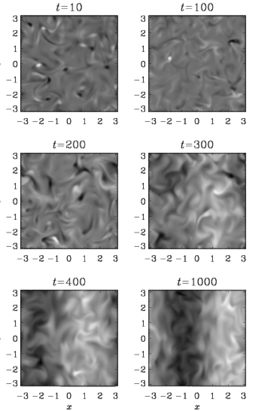
Figure 4: Gray-scale images of cross-sections of $B_{x}(x,y,0)$ for Run 3 at different times showing the gradual build-up of the large scale magnetic field after $t=300$. Dark (light) corresponds to negative (positive) values. Each image is scaled with respect to its min and max values.

Figure 5: The three magnetic field components averaged in the $x$ and $z$ directions at $t=1000$. Note the $90^{\circ}$ phase shift between $\langle{\overline{B}}_{x}\rangle(y)$ and $\langle{\overline{B}}_{z}\rangle(y)$, and that the functional form is nearly sinusoidal. Run 3.

Although our forcing is isotropic, one particular direction has been selected by the large scale magnetic field. In Runs 1 and 3 it was the $y$-direction, in Run 2 the $z$-direction, and in Run 5 the $x$-direction. Which direction is selected depends on fine details of the initially random condition. Nevertheless, it is not until the time of saturation that the final selection is established, as can be seen in Fig. 6 where we plot the magnetic energies of the mean field for the three possible directions, denoted by $E(K_{x})$, $E(K_{y})$, $E(K_{z})$. So,

$$E(K_{x})=\langle\langle\mbox{\boldmath$B$}{}\rangle_{yz}^{2}\rangle_{x},$$ (8)

$$E(K_{y})=\langle\langle\mbox{\boldmath$B$}{}\rangle_{xz}^{2}\rangle_{y},$$ (9)

$$E(K_{z})=\langle\langle\mbox{\boldmath$B$}{}\rangle_{xy}^{2}\rangle_{z},$$ (10)

where the subscripts denote the directions of averaging. Thus, for any direction $K$, say the $x$-direction, we define corresponding mean fields by averaging in the two perpendicular directions ($y$ and $z$ in this case), and then we calculate their mean squared value. The time of selection, i.e. when one of the three $E(K_{i})$ becomes dominant, is earlier in the large Reynolds number cases.

Figure 6: Magnetic energies (per volume) of those components of the large scale field whose wave vectors point in the $x$, $y$, or $z$ direction. Which of the three possible force-free solutions is selected in the end depends on chance.

A quantity of theoretical interest is the ratio $\langle\overline{\mbox{\boldmath$B$}}^{2}\rangle/\langle\mbox{\boldmath$B$}{}^{2}\rangle$, which characterizes the fraction of space occupied by the large scale field. Initially this ratio is just $\sim 2\%$ (for Run 3) and $\sim 0.7\%$ (for Run 5), but later it begins to level off near 80% (Fig. 7). Most likely real astrophysical dynamos are far less effective in producing such clean large scale fields, because in reality the helicity of the effective forcing will be far less than 100%. Nevertheless, it is important to notice that it is at least theoretically possible to achieve large scale field energies near or in excess of the kinetic energy, even though the magnetic Reynolds number is reasonably high.

Figure 7: Evolution of the ratio $\langle\overline{\mbox{\boldmath$B$}}\rangle^{2}/\langle\mbox{\boldmath$B$}{}^{2}\rangle$, for Runs 3 and 5. Note that strong large scale fields are obtained even for large magnetic Reynolds and Prandtl numbers.

We note that the phase of the large scale field may be drifting slowly as long as the large scale magnetic energy has not yet reached a fully steady state. In Run 3, for example, the phase was still drifting slowly in the $y$ direction (speed $\sim+1.5\eta k_{1}$), but then it began to settle after $t\approx 1000$.

3.3 Spectral helicity and energy transfer

The primary reason for the large scale field generation is related to magnetic helicity conservation. Once helicity is injected into the system, it tends to make the magnetic field also helical, as is seen from Fig. 8. For a closed or periodic system however the net magnetic helicity is conserved, except for diffusion at small scales, i.e.

$${{\rm d}{}\over{\rm d}{}t}\langle\mbox{\boldmath$A$}{}\cdot\mbox{\boldmath$B$}{}\rangle=-2\eta\langle\mbox{\boldmath$J$}{}\cdot\mbox{\boldmath$B$}{}\rangle.$$ (11)

Thus, if the magnetic field is to become helical, it must at first have equal amounts of positive and negative helicity. This feature, which is familiar in MHD (e.g. Seehafer 1996, Ji 1999), is also seen in hydrodynamical simulations (Biferale & Kerr 1995). At later times, however, magnetic diffusion can destroy magnetic helicity at small scales, leaving magnetic helicity of opposite sign at large scales. This is best described by the evolution equation of the magnetic helicity spectrum which can be derived from the Fourier transformed induction equation (3),

$${\partial\hat{\mbox{\boldmath$A$}{}}_{\mbox{\boldmath$k$}{}}\over\partial t}=\hat{\mbox{\boldmath${\cal E}$}{}}_{\mbox{\boldmath$k$}{}}-\eta\hat{\mbox{\boldmath$J$}{}}_{\mbox{\boldmath$k$}{}},$$ (12)

where hats and subscripts $k$ indicate three-dimensional Fourier transformation, and $\mbox{\boldmath${\cal E}$}{}=\mbox{\boldmath$u$}{}\times\mbox{\boldmath$B$}{}$ is the electromotive force. We write down the corresponding equation for the evolution of $\hat{\mbox{\boldmath$B$}{}}_{\mbox{\boldmath$k$}{}}=i\mbox{\boldmath$k$}{}\times\hat{\mbox{\boldmath$A$}{}}_{\mbox{\boldmath$k$}{}}$ and derive from these equations the evolution equation for $\hat{\mbox{\boldmath$A$}{}}_{\mbox{\boldmath$k$}{}}\cdot\hat{\mbox{\boldmath$B$}{}}_{\mbox{\boldmath$k$}{}}^{*}$, where asterisks denote complex conjugation. Note that this is gauge invariant, because adding a gradient to $\hat{\mbox{\boldmath$A$}{}}_{\mbox{\boldmath$k$}{}}$ corresponds to adding an $i\mbox{\boldmath$k$}{}\cdot\hat{\mbox{\boldmath$B$}{}}_{\mbox{\boldmath$k$}{}}^{*}$ term which vanishes, because the magnetic field is solenoidal. We denote the real parts of the shell-integrated spectra of $\hat{\mbox{\boldmath$A$}{}}_{\mbox{\boldmath$k$}{}}\cdot\hat{\mbox{\boldmath$B$}{}}_{\mbox{\boldmath$k$}{}}^{*}$ and $\hat{\mbox{\boldmath${\cal E}$}{}}_{\mbox{\boldmath$k$}{}}\cdot\hat{\mbox{\boldmath$B$}{}}_{\mbox{\boldmath$k$}{}}^{*}$ by $H_{\rm M}(k,t)$ and $S_{\rm M}(k,t)$, respectively, and obtain

$${\partial\over\partial t}H_{\rm M}(k,t)=2S_{\rm M}(k,t)-2\eta k^{2}H_{\rm M}(k,t).$$ (13)

Note that $\int H_{\rm M}(k,t)dk=\langle\mbox{\boldmath$A$}{}\cdot\mbox{\boldmath$B$}{}\rangle$ and, because of helicity conservation, $\int S_{\rm M}(k,t)dk=0$, so it makes sense to write Eq. (13) in the form

$${\partial\over\partial t}H_{\rm M}(k,t)=-{\partial\over\partial k}G_{\rm M}(k,t)-2\eta k^{2}H_{\rm M}(k,t),$$ (14)

where we have defined the spectral flux of helicity,

$$G_{\rm M}(k,t)=\int_{k}^{\infty}2S_{\rm M}(k^{\prime},t)\,{\rm d}{}k^{\prime},$$ (15)

which is plotted in Fig. 9 for different times. The magnetic helicity flux, $G_{\rm M}(k,t)$, is found to be always positive and its peak shifts from small scales ($k\approx 10$) at early times to large scales ($k=2-3$) at later times when the magnetic field becomes dynamically important. Positive magnetic helicity is being produced on the right of the maximum of $G_{\rm M}(k,t)$ and negative on the left; see Fig. 10.

Figure 8: Evolution of $-\langle\mbox{\boldmath$A$}{}\cdot\mbox{\boldmath$B$}{}\rangle/\langle\mbox{\boldmath$B$}{}^{2}\rangle$, compared with other magnetic length scales. Run 3.

Figure 9: Spectra of magnetic helicity flux at $t=10$, 30, and 60 (dot-dashed), 100 an 130 (solid), 160 and 200 (dashed), 300 (dotted), and for the time average between $t=600$ and 1000 (thick line).

Figure 10: Divergence of magnetic helicity flux, $S_{\rm M}(k)$, scaled by $k$, so the area under the positive and negative parts of the curve are the same when plotted in a lin-log plot. Because of resistive losses of positive magnetic helicity at small scales, the resulting magnetic helicity, $H_{\rm M}(k)$, is now dominated by negative helicity at large scales. The lower plot shows $H_{\rm M}(k)$, scaled by $k^{3}$ to show the contributions from small scales. Both spectra are time averages over the interval $600\leq t\leq 1000$.

In view of the realizability condition,

$$E_{\rm M}(k,t)\geq{\textstyle{1\over 2}}kH_{\rm M}(k,t)$$ (16)

(e.g. Moffatt 1978), the spectral magnetic helicity can be viewed as the driver of spectral magnetic energy: while small scale magnetic helicity is being destroyed, an equal amount gets into the large scales, and this must necessarily enhance the magnetic energy so as to satisfy (16). Indeed, in the present simulations the inequality (16) is almost saturated at all scales, except at intermediate scales $2\leq k\leq 4$; see Fig. 11.

Figure 11: Time-averaged spectra of kinetic and magnetic energy, as well as kinetic and magnetic helicity. Note that the magnetic energy exceeds the kinetic energy at $k=1$, and that the inequality (16) is almost saturated, except near $k=2$ and 3. The corresponding realizability condition for the kinetic helicity, on the other hand, is not very sharp. The dissipative cutoff wavenumber, $\langle\mbox{\boldmath$\omega$}{}^{2}/\nu^{2}\rangle^{1/4}$, is indicated by an arrow at the top.

In order to determine the dominant interactions leading to the generation of the large scale field at $k=1$ we now consider the spectral energy equation,

$${\partial\over\partial t}E_{\rm M}(k,t)=2T_{\rm M}(k,t)-2\eta k^{2}E_{\rm M}(k,t),$$ (17)

where the transfer function of magnetic energy, $T_{\rm M}(k,t)$, is the shell-integrated spectrum of the real part of $\hat{\mbox{\boldmath${\cal E}$}{}}_{\mbox{\boldmath$k$}{}}\cdot\hat{\mbox{\boldmath$J$}{}}_{\mbox{\boldmath$k$}{}}^{*}$. Since $\mbox{\boldmath${\cal E}$}{}=\mbox{\boldmath$u$}{}\times\mbox{\boldmath$B$}{}$, this corresponds really to a triple product,

$$\sum_{\mbox{\boldmath$k$}{}=\mbox{\boldmath$p$}{}+\mbox{\boldmath$q$}{}}(\hat{\mbox{\boldmath$u$}{}}_{\mbox{\boldmath$p$}{}}\times\hat{\mbox{\boldmath$B$}{}}_{\mbox{\boldmath$q$}{}})\cdot\hat{\mbox{\boldmath$J$}{}}_{\mbox{\boldmath$k$}{}}^{*},$$ (18)

where the skew product can also be written as $-\hat{\mbox{\boldmath$u$}{}}_{\mbox{\boldmath$p$}{}}\cdot(\hat{\mbox{\boldmath$J$}{}}_{\mbox{\boldmath$k$}{}}^{*}\times\hat{\mbox{\boldmath$B$}{}}_{\mbox{\boldmath$q$}{}})$, emphasizing that this term corresponds to the work done against the Lorentz force. In order to identify the dominant interactions we have calculated, in real space, the spectral transfer matrix

$$T_{\rm M}(k,p,q,t)=-\left\langle\mbox{\boldmath$u$}{}_{p}\cdot(\mbox{\boldmath$J$}{}_{k}\times\mbox{\boldmath$B$}{}_{q})\right\rangle,$$ (19)

where angular brackets denote volume averages and the subscripts $k$, $p$, and $q$ denote Fourier filtering around the corresponding wavenumber (by $\pm 1/2$). (In this notation $\langle\mbox{\boldmath$A$}{}_{k}\cdot\mbox{\boldmath$B$}{}_{k}\rangle$, for example, is exactly the same as the helicity spectrum.)

Figure 12: Spectral energy transfer function $T(k,p,t)$, normalized by $\langle\mbox{\boldmath$B$}{}^{2}\rangle$ for three different times, for $k=1$ and 2. Run 3.

In Fig. 12 we show $T(k,p)=\sum_{q}T(k,p,q)$, normalized by $\langle\mbox{\boldmath$B$}{}^{2}\rangle$ for the corresponding times, for $k=1$ and 2. This function shows that most of the energy of the large scale field at $k=1$ comes from velocity and magnetic field fluctuations at the forcing scale, $k=5$. At early times this is also true of the energy of the magnetic field at $k=2$, but at late times, $t=1000$, the gain from the forcing scale, $k=5$, has diminished, and instead there is now a net loss of energy into the next larger scale, $k=3$, suggestive of a direct cascade operating at $k=2$, and similarly at $k=3$.

The generation of large scale energy at $k=1$ through nonlocal inverse energy transfer is characteristic of the $\alpha$-effect in mean-field electrodynamics. In the following we shall pursue this analogy further. It should be emphasized, however, that without the simultaneous loss of energy at the next smaller scales (here $k=2$ and 3) through direct energy transfer the $k=1$ field would have been totally swamped by smaller scale fields. Thus, nonlinearity is quite crucial for this process to produce well defined large scale fields. Indeed, in the absence of the nonlinear term $\mbox{\boldmath$J$}{}\times\mbox{\boldmath$B$}{}$ in Eq. (2) the marked large scale pattern (Fig. 4) disappears within a turnover time. Recent numerical experiments have shown, however, that the ambipolar diffusion nonlinearity too leads to well defined large scale fields – even in the absence of the Lorentz force (Brandenburg & Subramanian 2000).

3.4 Mean-field interpretation

In this subsection we adopt the hypothesis that the large scale component of the field at wavenumber $k=1$ can be described in terms of mean-field theory. The magnetic field at other wavenumbers is ($k\geq 2$) is important for contributing to the $\alpha$-effect and the turbulent magnetic diffusivity, $\eta_{\rm t}$, but apart from that it is merely an extra source of noise as far as the dynamics of the large scale field is concerned. As we have seen in the previous section, this extra noise is automatically kept to a minimum due to direct cascade effects and transfer to kinetic energy during the saturation phase.

According to mean-field theory for non-mirror symmetric isotropic homogeneous turbulence with no mean flow the mean magnetic field is governed by the equation

$${\partial\over\partial t}\overline{\mbox{\boldmath$B$}}=\alpha\mbox{\boldmath$\nabla$}{}\times\overline{\mbox{\boldmath$B$}}+\eta_{\rm T}\nabla^{2}\overline{\mbox{\boldmath$B$}},$$ (20)

where bars denote the mean fields, $\alpha$ and $\eta_{\rm T}=\eta+\eta_{\rm t}$ are constants, and $\eta_{\rm t}$ is the turbulent magnetic diffusivity. In general, these coefficients are not constant and depend for example on the magnetic field. (In our particular case the local magnetic energy density is however approximately uniform.) Furthermore, since the magnetic field is strong, $\alpha$ and $\eta_{\rm t}$ should really be replaced by tensors, but we shall ignore this additional modification except that we shall allow $\alpha$ and $\eta_{\rm t}$ to vary slowly in time as the magnetic field approaches saturation. This simplified form of nonlinearity may be justified by noting that the mean magnetic field looks nearly sinusoidal (Fig. 5).

Equation (20) permits steady force-free solutions where the current helicity of the large scale field, $\overline{\mbox{\boldmath$J$}}\cdot\overline{\mbox{\boldmath$B$}}$ is given by $(\eta_{\rm T}/\alpha)\overline{\mbox{\boldmath$J$}}^{2}$. Apart from some common phase factor, the mean field depicted in Fig. 5 is given by $\overline{\mbox{\boldmath$B$}}(y)=(\sin y,0,\cos y)$, so $\overline{\mbox{\boldmath$J$}}=(-\sin y,0,-\cos y)$, corresponding to negative helicity, and therefore $\alpha$ must be negative. This is in agreement with mean-field theory which predicts that $\alpha$ is a negative multiple of the residual (kinetic minus current) helicity (e.g. Blackman & Chou 1997, Field, Blackman, & Chou 1999), which is positive in our case; see Table 1.

If the wavevector of the large scale field is $K_{y}$ (as in the case discussed above), Eq. (20) becomes

$$\dot{\overline{\mbox{\boldmath$B$}}}_{x}=+\alpha\overline{\mbox{\boldmath$B$}}_{z}^{\prime}+\eta_{\rm T}\overline{\mbox{\boldmath$B$}}_{x}^{\prime\prime},$$ (21)

$$\dot{\overline{\mbox{\boldmath$B$}}}_{z}=-\alpha\overline{\mbox{\boldmath$B$}}_{x}^{\prime}+\eta_{\rm T}\overline{\mbox{\boldmath$B$}}_{z}^{\prime\prime},$$ (22)

where dots and primes denote differentiation with respect to $t$ and $y$, respectively. Since $\alpha<0$, the solution can be written in the form

$$\overline{\mbox{\boldmath$B$}}_{x}(y,t)=b_{x}(t)\sin(y+\phi),$$ (23)

$$\overline{\mbox{\boldmath$B$}}_{z}(y,t)=b_{z}(t)\cos(y+\phi),$$ (24)

where $b_{x}(t)$ and $b_{z}(t)$ are positive functions of time that satisfy

$$\dot{b}_{x}=|\alpha|b_{z}-\eta_{\rm T}b_{x},$$ (25)

$$\dot{b}_{z}=|\alpha|b_{x}-\eta_{\rm T}b_{z}.$$ (26)

In a steady state $|\alpha|=\eta_{\rm T}$, and $b_{x}=b_{z}$. In order to find the actual values of $|\alpha|$ and $\eta_{\rm T}$ during both the saturated steady state and the growth phase we can do a simple experiment: suppose we put $b_{x}=0$ at some moment in time, then Eq. (25) would predict that $b_{x}$ starts to recover at the rate $|\alpha|b_{z}$, which allows us to estimate $\alpha$. In practice we put $b_{x}=0$ by subtracting ${\overline{B}}_{x}$ from the $x$ component of $B$ at a certain time and restart the simulation with that field.

In order to have a somewhat more precise estimate we need the solution to (25) and (26) for the initial condition $b_{x}(0)=0$;

$$b_{x}=e^{(|\alpha|-\eta_{\rm T})t}-e^{-(|\alpha|+\eta_{\rm T})t},$$ (27)

$$b_{z}=e^{(|\alpha|-\eta_{\rm T})t}+e^{-(|\alpha|+\eta_{\rm T})t},$$ (28)

where the amplitude is arbitrary in linear theory. Adding and subtracting (27) and (28) we can solve for $|\alpha|-\eta_{\rm T}$ and $|\alpha|+\eta_{\rm T}$, respectively. In terms of $|\alpha|$ and $\eta_{\rm T}$ separately, we have

$$|\alpha|={\textstyle{1\over 2}}{{\rm d}{}\over{\rm d}{}t}\left[+\ln(+b_{x}+b_{z})-\ln(-b_{x}+b_{z})\right],$$ (29)

$$\eta_{T}={\textstyle{1\over 2}}{{\rm d}{}\over{\rm d}{}t}\left[-\ln(+b_{x}+b_{z})-\ln(-b_{x}+b_{z})\right].$$ (30)

In practice we average the results of (29) and (30) over some 5–10 time units. We have applied this method to Runs 1–3 at times between $t=100-600$ and to Run 5 at times between $t=300-1600$ (Fig. 13). During these times the mean field was still evolving (Fig. 6), so at different times the mean magnetic field was different, which allows us to obtain the $\alpha(|\mbox{\boldmath$B$}{}|)$ dependence. We take into account the fact that during the experiment the actual field is only $1/\sqrt{2}$ of what it was before one of the two components of the mean field has been removed. We have then attempted a fit of the form

$$\alpha={\alpha_{0}\over 1+\alpha_{\rm B}\langle\overline{\mbox{\boldmath$B$}}^{2}\rangle/B_{\rm eq}^{2}},$$ (31)

where $B_{\rm eq}^{2}=\mu_{0}\rho_{0}\langle\mbox{\boldmath$u$}{}^{2}\rangle_{\rm sat}$. The result is shown in Fig. 14 and the coefficients $\alpha_{0}$ and $\alpha_{\rm B}$ are listed in Table 2. One should note, however, that Eq. (31) does not accurately represent the actual data of Run 5. Nevertheless, it is clear that $\alpha$-quenching is enhanced for large values of $R_{\rm m}$, which may be described by a fit of the form

$$\alpha_{\rm B}\approx(R_{\rm m,forc}/22)^{1.35}.$$ (32)

Such a steep dependence of $\alpha_{\rm B}$ on $R_{\rm m,forc}$ was suggested by Vainshtein et al. (1993), although his argument (see also Vainshtein & Cattaneo 1992) assumes the presence of strong small scale fluctuations (which is not the case here; see Fig. 7).

Figure 13: Example of the evolution of the mean fields, ${\overline{B}}_{y}$ and ${\overline{B}}_{z}$, after subtracting ${\overline{B}}_{y}$ from the actual field $B_{y}$ (left), and the corresponding results for $\alpha$ and $\eta_{\rm T}$ (right). The average values are indicated by horizontal lines. Run 5.

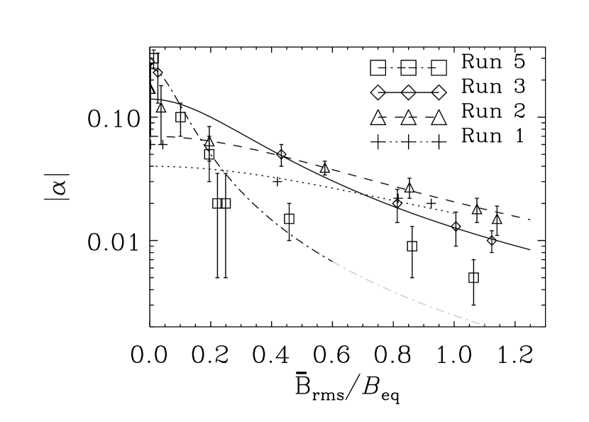
Figure 14: Results for $\alpha$ for different values of $R_{\rm m}$ using Eq. (29). The lines represent the fits described in the text.

In Fig. 15 we compare with the result for $\alpha$ obtained by just imposing a uniform magnetic field, $B_{0}\mbox{\boldmath$z$}{}$, and calculating $\alpha$ simply as

$$\alpha^{\rm imp}=(\langle\mbox{\boldmath$u$}{}\times\mbox{\boldmath$B$}{}\rangle)_{z}/B_{0}.$$ (33)

Each point in Fig. 15 corresponds to a different run with given field strength $B_{0}$, but otherwise the same parameters as in Runs 1–3 and 5. This method was frequently used in the past (e.g. Brandenburg et al. 1990, Tao et al. 1993, Cattaneo & Hughes 1996), but it is not a priori clear that one measures the same $\alpha$ as with the method explained above. Nevertheless, the two results appear to be qualitatively similar (cf. Figs 14 and 15) although there are some differences in the case where $R_{\rm m}$ is very large (Table 2). The same values of $\alpha_{\rm B}$ are confirmed by yet another method that is explained below in §3.6.

Figure 15: Results for $\alpha$ for different values of $R_{\rm m}$ using an imposed magnetic field. The lines represent the fits described in the text.

Table 2: Coefficients for the $\alpha$-quenching expressions for 4 runs with different values of $R_{\rm m}$.

	Run 1	Run 2	Run 3	Run 5
$R_{\rm m,lin}$	100	300	900	3600
$R_{\rm m,forc}$	20	60	180	700
$|\alpha_{0}|$	0.04	0.07	0.14	0.30
$\alpha_{\rm B}$	1.4	2.4	10	100
$|\alpha_{0}^{\rm imp}|$	0.040	0.076	0.092	0.035
$\alpha_{\rm B}^{\rm imp}$	1.3	4.3	14	35

Figure 16: Results for $\eta_{T}$ and $D_{T}$ for different values of $R_{\rm m}$. The lines represent the fits described in the text. In the plot of $\eta_{T}$ the asterisks denote $|\alpha|-\lambda$ for the $R_{\rm m,forc}=120$ run, which agrees reasonably well with $\eta_{T}$.

The only way a strongly $R_{\rm m}$-dependent $\alpha$ quenching can be compatible with the large scale field generation seen in the present simulations would be if $\eta_{\rm t}$ was also strongly quenched. [See Cattaneo & Vainshtein (1991) for two-dimensional simulations supporting the hypothesis of strong $\eta_{\rm t}$ quenching.] In Fig. 16 we compare the results obtained for $\eta_{\rm T}$ with the turbulent diffusion coefficient for a passive scalar. The passive scalar diffusion coefficient is obtained by simultaneously solving an additional equation for the concentration per unit mass, $c$,

$${{\rm D}\,{}c\over{\rm D}\,{}t}={1\over\rho}\mbox{\boldmath$\nabla$}{}\cdot\rho D\mbox{\boldmath$\nabla$}{}c,$$ (34)

where $D=\eta$ is chosen for Runs 1–3 and $D=2.5\eta$ for Run 5. The total (turbulent plus microscopic) passive scalar diffusion coefficient is obtained by measuring the rate at which a narrow gaussian distribution of $c$ widens as time goes on. The result is shown in the second panel of Fig. 16. Generally the suppression of $\eta_{\rm t}$ by magnetic fields is stronger than the suppression of $D_{\rm t}$. (For Run 3 $D_{\rm T}/D$ ranges between 40 for weak fields and 10 for strong fields.) We note that a dependence of the form

$$D_{\rm T}=D+D_{\rm t0}/(1+D_{\rm B}\langle|\overline{\mbox{\boldmath$B$}}|\rangle/B_{\rm eq})$$ (35)

seems to fit at least the $D_{\rm T}$ data better than a quadratic dependence. Unlike the results for $\alpha$, the dependence of $D_{\rm B}$ on Reynolds number is here less strong. In the fits shown in Fig. 16 a good fit is $D_{\rm B}=2$ for all three runs, and $D_{0}=0.02$, 0.035, and 0.06 for Runs 1, 2, and 3, respectively. Run 5 behaves differently, because in this large magnetic Prandtl number run there is no inertial range, and so we used $D_{0}=0.007$ and $D_{\rm B}=6$.

Determining $\eta_{\rm t}$ from dynamo simulations is notoriously difficult: $\eta_{\rm t}$ has to be determined simultaneously with $\alpha$ from the electromotive force, where $\eta_{\rm t}$ multiplies a derivative of the field, so it is numerically more noisy. Nevertheless, one sees from Fig. 16 that $\eta_{\rm t}$ is quenched by more than a factor of ten. However, the functional form cannot be established from our data. Using for $\eta_{\rm T}$ a similar fit formula as Eq. (35) we have $\eta_{\rm B}=16$ for all three runs, and $\eta_{\rm T0}=0.03$, 0.07, and 0.2 for Runs 1, 2, and 3, respectively, and $\eta_{\rm T0}=0.43$, $\eta_{\rm B}=60$ for Run 5. However, for strong magnetic fields, $\eta_{\rm T}$ levels off at a value of 0.01 (for Run 3) or 0.005 (for Run 5). These values are similar to the values of $\alpha$. Thus, $\alpha\approx\eta_{\rm T}k_{1}$, which means that the mean-field dynamo has turned into a marginally critical state, which is indeed to be expected. As a consistency check for the directly obtained values of $\eta_{\rm T}$ we use the time dependent growth rate $\lambda(t)$ and show $|\alpha|-\lambda$ (asterisks in Fig. 16) for Run 3. They agree reasonably well with $\eta_{T}$ (except near $\langle|\overline{\mbox{\boldmath$B$}}|\rangle=0.4B_{\rm eq}$), suggesting that (25) and (26) are approximately satisfied with the coefficients obtained above. Later in §3.6 we present a more accurate and self-consistent determination of the combined expression for $\alpha$ and $\eta_{\rm t}$-quenching by fitting solutions of Eq. (20) to the actual evolution of the mean field. Those results support a quadratic quenching formula for both $\alpha$ and $\eta_{\rm t}$.

3.5 Large scale separation

In some earlier exploratory models we forced the flow at $k=10$, which gave somewhat more room for the inverse cascade to develop, but less room for the direct cascade toward smaller wavenumbers. The latter means that the Reynolds number with respect to the forcing scale is smaller and the turbulent mixing properties, as quantified by the ratio $D_{\rm t}/D$, are poorer. Strong turbulent mixing was important in order to address the issue of Reynolds number dependent suppression of transport coefficients. In this subsection we shall accept poor mixing in favor of larger scale separation and hence a significantly larger subrange in which the inverse cascade can develop. Thus, we now force the flow at $k=30$ (Run 6).

After saturation is reached, which happens first at some intermediate scale, there is a wave of spectral energy propagating toward smaller $k$. This is similar to the results of closure models of Pouquet et al. (1976). However, unlike these models there does not seem to develop a $k^{-1}$ magnetic energy spectrum. Instead, there is only an envelope of the helicity wave that follows approximately a $k^{-1}$ powerlaw (Fig. 17). As before, there is a strong built-up of magnetic energy at the largest scale, $k=1$, combined with a subsequent suppression of energy at intermediate scales ($2\leq k\leq 20$). The ratio of the peak value at $k_{1}=1$ to the value of the secondary peak at the forcing scale $k_{\rm f}=30$ scales like $(k_{1}/k_{\rm f})^{-1}$ (Fig. 17). This is also the case in runs with $k_{\rm f}=5$ (Fig. 11).

Figure 17: Magnetic energy spectra for Run 6 with forcing at $k=30$. The times range from 0 (dotted line) to 10, 30, …, 290 (solid lines). The thick solid line gives the final state at $t=1000$. Note that at early times the spectra peaks at $k_{\max}\approx 7$. The $k^{-1}$ and $k^{+3/2}$ slopes are given for orientation as dash-dotted lines.

As a function of time, the spectral magnetic energy grows at the same rate at all values of $k$ until saturation is reached. During early times the magnetic spectra peak at $k_{\max}\approx 7$, which is also the wavenumber that reaches equipartition first, but then the field at this wavenumber decays to a somewhat smaller value while the contributions from the next smaller $k$ grow and subsequently decay; see Fig. 18. Finally, when the energy at $k=1$ reaches equipartition the energy of all larger $k$s becomes suppressed.

Figure 18: Evolution of spectral magnetic energy for selected wavenumbers in a simulation with forcing at $k=30$.

Although a comparison with mean-field theory may be inappropriate, it is interesting to note that the existence of a $k_{\max}$ is predicted from the theory of $\alpha^{2}$ dynamos in infinite media (Moffatt 1978). The dispersion relation is

$$\lambda=|\alpha|k-\eta_{\rm T}k^{2},$$ (36)

where $\lambda$ is the growth rate. Maximum growth occurs at wavenumber

$$k_{\max}={\textstyle{1\over 2}}|\alpha|/\eta_{\rm T},$$ (37)

and there the maximum growth rate is

$$\lambda_{\max}={\textstyle{1\over 2}}|\alpha|k_{\max}.$$ (38)

Since $k_{\max}$ and $\lambda_{\max}$ can be measured, we can determine

$$|\alpha|=2\lambda_{\max}/|k_{\max},\quad\eta_{\rm T}=\lambda_{\max}/|k_{\max}^{2}$$ (39)

during the growth phase of the dynamo. With $k_{\max}=7$ (Fig. 18) and $\lambda_{\max}=0.07$ (Fig. 17) we have $|\alpha|=0.02$ and $\eta_{\rm T}=0.0014$. In this case, the forcing occurs essentially in the dissipation range, so the turbulence has therefore poor mixing properties ($\eta_{\rm T}/\eta=1.4$). The value of $\alpha$ is about 7 times smaller than that of Run 3 during the kinematic regime, which seems reasonable.

In the nonlinear regime there are marked differences between mean-field theory and simulations. Using a nonlinear mean-field model of the inverse cascade with $\alpha$-effect, Galanti, Sulem, & Gilbert (1991) found significant power at $k\geq 2$, which is in contrast to the behavior seen in Fig. 17. Consequently, the mean fields of Galanti, Gilbert, & Sulem (1990) look much less sinusoidal than in the simulations (Fig. 5). If one wanted to model this within the framework of an $\alpha$-effect one would need to invoke a scale-dependent $\alpha$ integral kernel, where the dominant contributions to $\alpha$ come only from the largest scale of the system (Brandenburg & Sokoloff 2000).

3.6 Reynolds number dependence and magnetic helicity

In this section we first discuss to which extent our results are affected by the limited resolution and finite magnetic Reynolds number. We then show that magnetic helicity conservation implies slow saturation of helical magnetic fields, and that this features is quantitatively reproduced by a mean-field model with $R_{\rm m}$-dependent quenching of $\alpha$ and $\eta_{t}$.

In Fig. 19 we show energy spectra of the magnetic field for three values of $R_{\rm m}$. The three curves differ by a certain factor, but are otherwise essentially the same at small wavenumbers. The main difference is, as expected, at the smaller scales: the spectra for large $R_{\rm m}$ begin to show signs of an inertial range for values of $k$ larger than the forcing wavenumber.

Figure 19: Comparison of time averaged magnetic energy spectra for Runs 1–3 ($t=600-1000$) and Run 5 ($t=1600$). To compensate for different field strengths and to make the spectra overlap at large scales, two of the three spectra have been multiplied by a scaling factor ($\times 3.4$ for Run 5, $\times 2$ for Run 2 and $\times 5$ for Run 1). There are signs of a gradual development of an inertial subrange for wavenumbers larger than the forcing scale. The $k^{-5/3}$ slope is shown for orientation. The dissipative magnetic cutoff wavenumbers, $k_{\rm d}=\langle\mbox{\boldmath$J$}{}^{2}/\eta^{2}\rangle^{1/4}$, are indicated by arrows at the top.

Although the magnetic energy spectra of the statistically steady state seem to show convergence to a spectrum roughly compatible with $k^{-5/3}$, there are some serious concerns about the timescale on which such a steady state is achieved. As was first pointed out by Berger (1984), in a closed box (periodic or perfectly conducting) there is an upper bound on the rate of change of the magnetic helicity. This is relevant, because the fields that are generated in the simulations have strong magnetic helicity: $\langle\mbox{\boldmath$A$}{}\cdot\mbox{\boldmath$B$}{}\rangle/\langle\mbox{\boldmath$B$}{}^{2}\rangle\approx-0.8/k_{1}$ (Fig. 8). Most of the magnetic helicity is in the large scales (Fig. 11). In order to build up the helicity at large scales we have to destroy magnetic helicity at small scales (Fig. 9).

Open boundary conditions would help to get rid of magnetic helicity (cf. Blackman & Field 2000), which may well be an important factor in more realistic simulations (e.g. Glatzmaier & Roberts 1995, Brandenburg et al. 1995). However, the present simulations are for closed boxes and yet they do show strong fields, so we need to understand whether and how they have been affected by this constraint.

The rate at which magnetic helicity can change, see Eq. (11), is constrained by the Schwarz inequality,

$$\left|{{\rm d}{}\over{\rm d}{}t}\langle\mbox{\boldmath$A$}{}\cdot\mbox{\boldmath$B$}{}\rangle\right|=2\eta\,|\langle\mbox{\boldmath$J$}{}\cdot\mbox{\boldmath$B$}{}\rangle|\leq 2\eta\,J_{\rm rms}B_{\rm rms}$$ (40)

(Berger 1984, Moffatt & Proctor 1985). In forced systems it is common (albeit not necessary) that the energy ($B_{\rm rms}^{2}$) and dissipation rate ($\eta J_{\rm rms}^{2}$) are independent of the Reynolds number. However, this would imply that the rate of change of $\langle\mbox{\boldmath$A$}{}\cdot\mbox{\boldmath$B$}{}\rangle$ is limited resistively by a term proportional to $\eta^{1/2}$. In our simulations, $\langle\mbox{\boldmath$J$}{}\cdot\mbox{\boldmath$B$}{}\rangle/(J_{\rm rms}B_{\rm rms})$ has a maximum of $\sim 0.25$ (see Table 1), so this limit does not seem to be saturated. Another estimate for the helicity dissipation is obtained by assuming that the magnetic spectrum has powerlaw behavior with $E_{\rm M}(k)\sim k^{-n}$ for $k<k_{\rm d}$. The value of $k_{\max}$ follows by assuming that the Joule dissipation is independent of $\eta$, which yields $k_{\rm d}\sim\eta^{-1/(3-n)}$ ($\sim\eta^{-3/4}$ for $n=5/3$). The helicity dissipation is then proportional to $k_{\rm d}^{-1}\sim\eta^{1/(3-n)}$, which always tends to zero for small values of $\eta$. For $n=5/3$ the magnetic helicity dissipation scales like $\eta^{3/4}$, which is faster than Berger’s limit.

There is a related and even more important consequence of helicity conservation. In a steady state, $\langle\mbox{\boldmath$A$}{}\cdot\mbox{\boldmath$B$}{}\rangle$, which is gauge invariant and therefore physically meaningful, must be constant, and hence $\langle\mbox{\boldmath$J$}{}\cdot\mbox{\boldmath$B$}{}\rangle\rightarrow 0$. Thus, although we are going to generate a strong large scale field with significant current helicity in the large scales, the net current helicity must actually vanish. This can only happen if there is an equal amount of small scale current helicity of opposite sign, i.e.

$$\langle\mbox{\boldmath$j$}{}\cdot\mbox{\boldmath$b$}{}\rangle\approx-\langle\overline{\mbox{\boldmath$J$}}\cdot\overline{\mbox{\boldmath$B$}}\rangle\quad\mbox{(in the steady state)},$$ (41)

where angular brackets denote volume averages, bars denote the large scales at $k=1$, and lower characters refer to contributions from all higher wavenumbers. The spectrum of the magnetic helicity is $k^{2}$ times steeper than that of the current helicity, so $\langle\mbox{\boldmath$a$}{}\cdot\mbox{\boldmath$b$}{}\rangle\approx\langle\mbox{\boldmath$j$}{}\cdot\mbox{\boldmath$b$}{}\rangle/k_{\rm f}^{2}$, and therefore $|\langle\mbox{\boldmath$a$}{}\cdot\mbox{\boldmath$b$}{}\rangle|\ll|\langle\overline{\mbox{\boldmath$A$}}\cdot\overline{\mbox{\boldmath$B$}}\rangle|$.

In the following we estimate the evolution of the energy density of the large scale field, $\overline{\mbox{\boldmath$B$}}^{2}$, using the fact that in the present simulations a large fraction of the magnetic energy is contained in the large scale field (Fig. 7) and that magnetic helicity is strong (Fig. 8). This would be too ideal an assumption for astrophysical settings, but it is adequate for describing our present simulations. Thus, we may set

$$k_{1}\langle\mbox{\boldmath$A$}{}\cdot\mbox{\boldmath$B$}{}\rangle\approx k_{1}\langle\overline{\mbox{\boldmath$A$}}\cdot\overline{\mbox{\boldmath$B$}}\rangle\approx-\langle\overline{\mbox{\boldmath$B$}}^{2}\rangle\approx\langle\overline{\mbox{\boldmath$J$}}\cdot\overline{\mbox{\boldmath$B$}}\rangle/k_{1}.$$ (42)

For clarity we retain here the $k_{1}$ factors, even though they are one. Using Eq. (11) this yields

$${{\rm d}{}\over{\rm d}{}t}\langle\overline{\mbox{\boldmath$B$}}^{2}\rangle\approx-2\eta k_{1}^{2}\langle\overline{\mbox{\boldmath$B$}}^{2}\rangle+2\eta k_{1}|\langle\mbox{\boldmath$j$}{}\cdot\mbox{\boldmath$b$}{}\rangle|,$$ (43)

which has the solution

$$\langle\overline{\mbox{\boldmath$B$}}^{2}\rangle\approx 2\eta k_{1}e^{-2\eta k_{1}^{2}t}\int_{t_{\rm sat}}^{t}e^{2\eta k_{1}^{2}t^{\prime}}|\langle\mbox{\boldmath$j$}{}\cdot\mbox{\boldmath$b$}{}\rangle|\,{\rm d}{}t^{\prime},$$ (44)

which is expected to apply after the time of saturation, $t=t_{\rm sat}$, when $\langle\mbox{\boldmath$j$}{}\cdot\mbox{\boldmath$b$}{}\rangle$ is approximately constant, so

$$\langle\overline{\mbox{\boldmath$B$}}^{2}\rangle\approx{|\langle\mbox{\boldmath$j$}{}\cdot\mbox{\boldmath$b$}{}\rangle|\over k_{1}}\left[1-e^{-2\eta k_{1}^{2}(t-t_{\rm sat})}\right].$$ (45)

To a good approximation we may assume $\langle\mbox{\boldmath$j$}{}\cdot\mbox{\boldmath$b$}{}\rangle\approx\rho_{0}\langle\mbox{\boldmath$\omega$}{}\cdot\mbox{\boldmath$u$}{}\rangle$. This means that the ‘residual helicity’ (Pouquet et al. 1976), $\langle\mbox{\boldmath$\omega$}{}\cdot\mbox{\boldmath$u$}{}\rangle-\langle\mbox{\boldmath$j$}{}\cdot\mbox{\boldmath$b$}{}\rangle/\rho_{0}$, is small, which is indeed consistent with the present data and also with a results of Brandenburg & Subramanian (2000), who used the ambipolar diffusion model of Subramanian (1999). The kinetic helicity can be approximated by $\langle\mbox{\boldmath$\omega$}{}\cdot\mbox{\boldmath$u$}{}\rangle\approx k_{\rm f}\langle\mbox{\boldmath$u$}{}^{2}\rangle$, and so the final field strength, $B_{\rm fin}$, is given by

$$B_{\rm fin}^{2}\approx{|\langle\mbox{\boldmath$j$}{}\cdot\mbox{\boldmath$b$}{}\rangle|\over k_{1}}\approx\rho_{0}{|\langle\mbox{\boldmath$\omega$}{}\cdot\mbox{\boldmath$u$}{}\rangle|\over k_{1}}\approx\rho_{0}\langle\mbox{\boldmath$u$}{}^{2}\rangle{k_{\rm f}\over k_{1}}\equiv B_{\rm eq}^{2}{k_{\rm f}\over k_{1}},$$ (46)

For Runs 1–3 and 5–7, the ratio of the actual values of $B_{\rm fin}$ to those anticipated from Eq. (46) are 0.61, 0.76, 0.85, 1.16, 0.74, and 0.36. In the large $R_{\rm m}$ cases (Runs 3 and 5) the ratio is close to one, confirming thus the assumption of small residual helicity in the saturated state.

The resistively limited growth of $\overline{\mbox{\boldmath$B$}}$ has immediate consequences for $\alpha$. The evolution equation for $\langle\overline{\mbox{\boldmath$A$}}\cdot\overline{\mbox{\boldmath$B$}}\rangle$ can be derived from Eq. (20),

$${{\rm d}{}\over{\rm d}{}t}\langle\overline{\mbox{\boldmath$A$}}\cdot\overline{\mbox{\boldmath$B$}}\rangle=2\alpha\langle\overline{\mbox{\boldmath$B$}}^{2}\rangle-2\eta_{\rm T}\langle\overline{\mbox{\boldmath$J$}}\cdot\overline{\mbox{\boldmath$B$}}\rangle.$$ (47)

In the strongly helical case considered here the magnetic helicity of the large scale field, $\langle\overline{\mbox{\boldmath$A$}}\cdot\overline{\mbox{\boldmath$B$}}\rangle$, is very nearly equal to $\langle\mbox{\boldmath$A$}{}\cdot\mbox{\boldmath$B$}{}\rangle$, so the right hand sides of (11) and (47) must be approximately equal, which leads to

$$|\alpha|-\eta_{\rm T}k_{1}\approx\eta|\langle\mbox{\boldmath$J$}{}\cdot\mbox{\boldmath$B$}{}\rangle|/\langle\overline{\mbox{\boldmath$B$}}^{2}\rangle.$$ (48)

In order to check this relation we plot the two sides of (48) versus time (Fig. 20), where $\eta_{\rm T}=\eta+\eta_{\rm t}$ and $|\alpha|-\eta_{\rm t}k_{1}$ has been obtained directly from $\mbox{\boldmath${\cal E}$}{}=\mbox{\boldmath$u$}{}\times\mbox{\boldmath$B$}{}$ assuming $\overline{\mbox{\boldmath${\cal E}$}}=\alpha\overline{\mbox{\boldmath$B$}}-\eta_{\rm t}\overline{\mbox{\boldmath$J$}}$ which, for fully helical mean fields, leads to

$$|\alpha|-\eta_{\rm t}k_{1}=|\langle\overline{\mbox{\boldmath${\cal E}$}}\cdot\overline{\mbox{\boldmath$B$}}\rangle|/\langle\overline{\mbox{\boldmath$B$}}^{2}\rangle.$$ (49)

(Note that here $\eta_{\rm t}$ enters, not $\eta_{\rm T}$. Recall also that in our case $\alpha<0$, so $\langle\overline{\mbox{\boldmath${\cal E}$}}\cdot\overline{\mbox{\boldmath$B$}}\rangle<0$.) The condition (48) on $\alpha$ reflects the fact that the growth of the large scale field is limited by the microscopic resistivity, as seen already from Eq. (45). Note, however, that this statement only applies to the present case of strong helicity and closed or periodic boxes.

Figure 20: Comparison of $|\alpha|-\eta_{\rm T}k_{1}$ with $\eta\langle\mbox{\boldmath$J$}{}\cdot\mbox{\boldmath$B$}{}\rangle/\langle\overline{\mbox{\boldmath$B$}}^{2}\rangle$ and $\eta\exp[-2\eta k_{1}^{2}(t-t_{\rm sat})]$. Note that $|\alpha|-\eta_{\rm T}k_{1}$ follows very closely the resistively dominated limit. Notice also the relatively large noise level in $|\alpha|-\eta_{\rm T}$. Run 3.

There have been previous attempts to incorporate the conservation of helicity into the expression for $\alpha$, which led to a dynamical dependence of $\alpha$ on time and field strength (Kleeorin, Rogachevskii, & Ruzmaikin 1995, Kleeorin et al. 2000). In the following we point out, however, that the helicity constraint, which leads to the prolonged saturation phase, is well described in terms of an $\alpha^{2}$-dynamo with resistively dominated quenching functions for both $\alpha$ and $\eta_{\rm t}$, i.e.

$$\alpha={\alpha_{0}\over 1+\alpha_{B}\overline{\mbox{\boldmath$B$}}^{2}\!/B_{\rm eq}^{2}},\quad\eta_{\rm t}={\eta_{\rm t0}\over 1+\eta_{B}\overline{\mbox{\boldmath$B$}}^{2}\!/B_{\rm eq}^{2}},$$ (50)

where $\alpha_{B}=\eta_{B}$ is assumed. Using the fact that the magnetic energy density of the mean field, $\overline{\mbox{\boldmath$B$}}^{2}$, is approximately uniform we can write Eq. (20) in the form

$${{\rm d}{}\over{\rm d}{}t}\left({\textstyle{1\over 2}}\overline{\mbox{\boldmath$B$}}^{2}\right)={|\alpha_{0}|k_{1}-\eta_{\rm t0}k_{1}^{2}\over 1+\alpha_{B}\overline{\mbox{\boldmath$B$}}^{2}\!/B_{\rm eq}^{2}}\overline{\mbox{\boldmath$B$}}^{2}-\eta k_{1}^{2}\overline{\mbox{\boldmath$B$}}^{2}.$$ (51)

There is a steady solution with

$$\alpha_{B}\overline{\mbox{\boldmath$B$}}^{2}/B_{\rm eq}^{2}=\lambda/\eta k_{1}^{2},$$ (52)

where

$$\lambda=|\alpha_{0}|k_{1}-\eta_{\rm T0}k_{1}^{2}$$ (53)

is the kinematic growth rate of the dynamo and $\eta_{\rm T0}=\eta+\eta_{\rm t0}$. The time dependent equation (51) can be integrated to give the solution in the form

$$\overline{\mbox{\boldmath$B$}}^{2}/(1-\overline{\mbox{\boldmath$B$}}^{2}\!/B_{\rm fin}^{2})^{1+\lambda/\eta k_{1}^{2}}=B_{\rm ini}^{2}\,e^{2\lambda t},$$ (54)

where $B_{\rm ini}$ is the initial field strength and $B_{\rm fin}$ is the final field strength which is given by Eq. (52). The parameters $B_{\rm ini}$ and $B_{\rm fin}$ can be obtained from Fig. 1. The kinematic growth rate $\lambda$ is the same for small and large scale fields and can hence be taken from Table 1. We emphasize that there is excellent agreement between the results of the simulation and the solution (54); see Fig. 21.

Figure 21: Evolution of $\langle\overline{\mbox{\boldmath$B$}}^{2}\rangle$ for Runs 1–3 and 5–7 (solid lines), compared with the solution (54) of the mean-field dynamo equations using resistively dominated $\alpha$ and $\eta_{\rm t}$ quenchings (dotted lines)

Having obtained $\lambda$ and $B_{\rm fin}$ from the simulation we can use Eq. (52) to find for $\alpha_{B}$ and $\eta_{B}$ the result

$$\alpha_{B}=\eta_{B}={\lambda\over\eta k_{1}^{2}}\left({B_{\rm eq}\over B_{\rm fin}}\right)^{2}.$$ (55)

Note that $\alpha_{B}$ and $\eta_{B}$ are proportional to $1/\eta$, which implies $R_{\rm m}$-dependent $\alpha$ and $\eta_{\rm t}$ quenchings. The results for $\alpha_{B}=\eta_{B}$ are summarized in Table 3 for different runs.

To a good approximation $B_{\rm fin}^{2}/B_{\rm eq}^{2}\approx k_{\rm f}/k_{1}$, see Eq. (46), so we expect $\alpha_{B}\approx\lambda/(\eta k_{1}k_{\rm f})$. Since $\lambda\approx 0.3\times u_{\rm rms}/\ell_{\rm f}$ we have

$$\alpha_{B}\approx{0.3\over(2\pi)^{2}}\,{u_{\rm rms}L\over\eta}\approx 0.01\times R_{\rm m,lin}.$$ (56)

Thus, $\alpha_{B}$ should scale with the magnetic Reynolds number based on the box scale – not the forcing scale. The difference is particularly evident when comparing with Run 6 where the forcing wavenumber is six times larger than in the other runs. For comparison we list in Table 3 also $R_{\rm m,lin}/100$ and $R_{\rm m,forc}/20$. The agreement between Eqs. (55) and (56) is generally good, except for Run 7 where $\alpha_{\rm B}$ is larger than expected. This is probably because in this run with a small value of $\nu/\eta$ and small $R_{\rm m}$ the value of $B_{\rm fin}$ is smaller than expected from Eq. (46); see Eq. (55).

In Table 3 we also give for completeness the values of $B_{\rm ini}$. Together with the values of $\eta$ and $\lambda$ in Table 1 all the data entering Eq. (54) are now specified. It should be mentioned that the value of $B_{\rm ini}$ is obtained from a fit and is only roughly comparable to the actual seed magnetic field in the simulation, where different initial structures are possible.

Table 3: Coefficients for the $\alpha$-quenching expression obtained from Eq. (55) for runs with different values of magnetic Reynolds number. Note the rough agreement between the values of $R_{\rm m,lin}/100$ and $\alpha_{\rm B}$ for all runs except Run 7.

	${\displaystyle{R_{\rm m,lin}\over 100}}$	${\displaystyle{R_{\rm m,forc}\over 20}}$	$\alpha_{\rm B}$	$B_{\rm fin}$	$B_{\rm ini}$
Run 1	1	1	1.4	0.16	$3\times 10^{-8}$
Run 2	3	3	3.9	0.25	$3\times 10^{-9}$
Run 3	9	9	9.3	0.34	$2\times 10^{-9}$
Run 5	35	35	30	0.27	$4\times 10^{-11}$
Run 6	5	1	4.6	0.25	$4\times 10^{-11}$
Run 7	1	1	2.8	0.16	$1\times 10^{-9}$

For weak fields Eq. (54) gives the usual exponential growth, $|\overline{\mbox{\boldmath$B$}}|=B_{\rm ini}\exp(\lambda t)$. For strong fields we recover Eq. (45) with $t_{\rm sat}=\lambda^{-1}\ln(B_{\rm fin}/B_{\rm ini})$ in the limit $\lambda\gg\eta k_{1}^{2}$.

3.7 Large magnetic Prandtl numbers

The magnetic helicity constraint becomes more important as the magnetic Reynolds number is increased. So far we have mainly considered the case where $\nu/\eta=1$. In the sun and many other astrophysical bodies, $\nu/\eta\ll 1$, but in the galaxy $\nu/\eta\gg 1$ (e.g. Kulsrud & Andersen 1992). This may lead to a magnetic energy spectrum peaking at small scales (Kulsrud & Andersen 1992). However, although viscous damping will dissipate energy at small scales (Chandran 1998, Kinney et al. 1998), there is some recent evidence that the inverse cascade may no longer operate (Maron 2000). These results have been obtained in the absence of net helicity. It will therefore be interesting to see whether in the presence of net helicity an inverse cascade is still possible when $\nu/\eta\gg 1$.

In a preliminary attempt to clarify this question we have carried out simulations for $\nu/\eta=20$ (mainly by increasing the viscosity to $\nu=0.02$; Run 4) and $\nu/\eta=100$ (where the magnetic diffusivity was lowered to $\eta=2\times 10^{-4}$; Run 5). The viscous cutoff wavenumber is then around 5, i.e. at the forcing scale, and the magnetic cutoff wavenumbers are 25 and 72, respectively. The resolution for Run 5 may be insufficient and discretisation errors must play a role at small scales, but the images of the current density look reasonable (see below) and the evolution of the large scale field is also in agreement with expectations (§3.6).

Figure 22: Spectra of magnetic and kinetic energy and helicity for a large magnetic Prandtl number at early and late times. $\nu=0.02$, $\eta=2\times 10^{-4}$.

As seen from Fig. 22 the magnetic energy spectrum does indeed peak at large wavenumbers initially, although the magnetic energy spectrum does not scale like $k^{3/2}$ (Kulsrud & Andersen 1992). Instead, the spectrum is close to $k^{1/3}$, which was also found during the kinematic stage of convective dynamos (Brandenburg et al. 1996). However, this result is inconclusive, because it could be an artifact of the lack of an inertial range in this run. In any case, at large wavenumbers the magnetic energy exceeds the kinetic energy, although at later times the kinetic energy is increased somewhat by magnetic forces. Especially at later times the magnetic energy is no longer dominated by small scales and the spectrum falls off more like $k^{-5/3}$. The convergence to this powerlaw is evident when comparing Runs 3, 4, and 5 (Fig. 23). Most importantly, there are now clear signs of an inverse cascade; see Fig. 24.

Figure 23: Comparison of the magnetic energy spectra for Runs 3, 4 and 5. The magnetic cutoff wavenumbers are 25, 26, and 72, as indicated by arrows at the top.

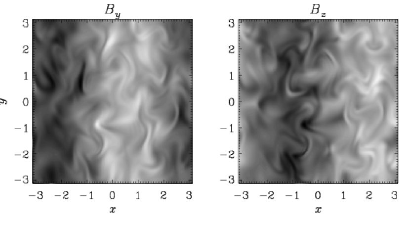
Figure 24: Images of the $B_{y}$ and $B_{z}$ components of the magnetic field in an arbitrarily chosen $xy$ plane. Run 5, $t=1600$.

In these runs with large magnetic Prandtl number the current density shows strong filamentary structures that tend to be aligned with the local magnetic field direction, as seen in Fig. 25. The resulting anisotropy affects particularly the small scales (Goldreich & Sridhar 1997, Maron 2000). Note that this type of anisotropy cannot be captured by closure models (e.g. Pouquet et al. 1976).

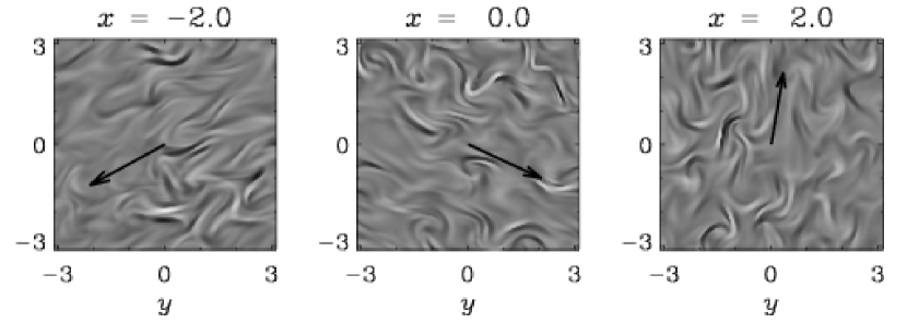
Figure 25: Images of the current density, $J_{x}$, in the plane of the large scale magnetic field. The field direction is shown as a vector. Run 5, $t=1600$.

The main shortcoming of the present large Prandtl number calculations is that the viscous dissipation cutoff wavenumber is so small that it lies in the range of the forcing scale, so no inertial range in the kinetic energy is possible. At the same time, of course, the range of scales available to the magnetic field is still not large enough to establish a $k^{3/2}$ scaling at early times.

4 Conclusions

The main conclusion to be drawn from this work is that in the presence of net magnetic helicity there is a gradual built-up of a nearly force-free magnetic field at the largest possible scale of the system. In our periodic calculations this corresponds to a sinusoidal one-dimensional Beltrami field, e.g. $\overline{\mbox{\boldmath$B$}}\sim(\cos z,\sin z,0)$, which is of course locally strongly distorted by the turbulence. Nevertheless, the presence of the large scale field is clearly seen without averaging (Fig. 4). We emphasize that this result is numerically robust: the relative dominance of magnetic energy at the smallest wavenumber is independent of resolution (Fig. 19) and independent of the degree of scale separation (Fig. 17). So, the effect is seen equally well at resolutions ranging from $30^{3}$ to $120^{3}$ meshpoints, and at forcing wavenumbers ranging from 5 to 30. However, the time it takes to establish such large scale fields increases with the ohmic diffusion time. We also note that the results are not very sensitive to the choice of the forcing function: a forcing function that is nearly delta-correlated in space, but still strongly helical, yields very similar results. In the absence of net helicity, however, no large scale field is generated. Likewise, if the forcing is made non-helical the large scale field disappears.

An important property of the turbulence is that once the large scale field is established, it can suppress magnetic energy on scales smaller than the largest one. This leads to something like a ‘self-cleaning’ processes. This is also seen in histograms of the magnetic field which are, for the present simulations, more nearly gaussian (with one hump perpendicular to the field, and two in the direction of the field). This is similar to other simulations with large scale dynamo action (see Brandenburg et al. 1995), but very different from simulations of small scale dynamo action where the histograms of the field components show stretched exponentials (Brandenburg et al. 1996), which can also be seen in the present simulations, but only at early times.

Our simulations show that most of the energy input to the large scale field comes from small scales. This type of nonlocal spectral energy transfer is suggestive of an $\alpha$-effect that could be responsible for the field generation, rather than a local inverse cascade, which transports energy from $k=2$ to $k=1$, for example. Although a local inverse cascade seems to occur at early times, i.e. before the magnetic field is fully established, once the field is strong the magnetic energy at $k=2$ is actually cascaded to $k=3$ and/or transferred to kinetic energy, both of which are probably important for the ‘self-cleaning’ processes. A sketch of the anticipated energy transfer properties is given in Fig. 26.

Figure 26: Sketch illustrating direct and inverse cascade processes in helical MHD turbulence.

We point out that the present simulations must not be regarded as local in the sense of representing only a small chunk of a larger system, because the field structure depends crucially on the size of the box. Instead, they should be viewed as global within the geometry considered. With other boundary conditions or in different geometries the shape of the large scale field will be different. In the case of a sphere, for example, no perfectly force-free field is possible, but the field may be nearly force-free. An example may be the field obtained in hydromagnetic calculations with $\alpha$-effect (Proctor 1977), where field saturation occurs through the Lorentz force of the large scale field. In these calculations the magnetic saturation field strength is relatively large, which reflects the fact that the field is indeed nearly force-free.

It should be emphasized that the overall growth of the large scale field and the saturation phase of the dynamo are well described by a simple $\alpha^{2}$-dynamo with $\alpha$ and $\eta_{\rm t}$ coefficients that are quenched in a $R_{\rm m}$-dependent fashion; see Eqs. (50) and (55). The reason such a dynamo can still saturate is because of the presence of microscopic diffusion, and it is this what causes the saturation to happen so slowly. The excellent agreement in the evolution toward saturation between both the simulation and the mean-field model is an indication that the simple quadratic quenching formula is actually correct. For example a cubic nonlinearity (Moffatt 1972, Rüdiger 1974) would lead to different behavior and would not have the correct resistive relaxation asymptotics consistent with helicity conservation (Brandenburg 2000).

The slow resistive field evolution past equipartition has become particularly clear in Run 5, where the final selection of the large scale field structure occurred rather late (after $t\approx 1200$, corresponding to about 100 turnover times; Fig. 6). By contrast, in Run 3, where the magnetic Reynolds number was about 6 times smaller, the large scale field was fully developed by the time $t\approx 400$, corresponding to about 50 turnover times. In stars the typical magnetic Reynolds numbers are at least another six orders of magnitude larger than in Run 5, so a large scale field, if generated by an $\alpha$-effect, would require $\sim 10^{8}$ turnover times or $\sim 3\times 10^{6}\,{\rm yr}$ (assuming a turnover time of 10 days). In the case of the sun this estimate would be reduced by another factor of 100 (Brandenburg et al. 2000), because differential rotation contributes to non-helical field generation, so the resulting fields are only partially subject to the helicity constraint. Since even the youngest protostars are older than $3\times 10^{4}\,{\rm yr}$ the $\alpha\omega$-dynamo may still be responsible for field generation in these bodies. For galaxies, on the other hand, the magnetic Reynolds numbers are by another seven orders of magnitude larger than in stars, making here the case for an $\alpha\omega$-dynamo more doubtful. However, this assumes that the conclusions from models with closed or periodic boundaries apply to galaxies, and that the microscopic resistivity is not enhanced during reconnection [see Ji et al. (1998) for anomalous resistivities in a laboratory reconnection experiment].

There is now also some evidence that in oscillatory dynamos of $\alpha\omega$-type the cycle period is not strongly affected by the helicity timescale constraint (Brandenburg et al. 2000). This could be related to the fact that with shear the large scale field is no longer fully force-free and that in that case the turbulent magnetic diffusivity is only partially suppressed (Gruzinov & Diamond 1996). However, the case for $\alpha\omega$-dynamo action in stars, galaxies or accretion discs is by no means settled. Firstly, proposals have been made for nonhelical large scale dynamo action (Vishniac & Cho 2000, Zheligovsky, Podvigina, & Frisch 2000), which may avoid the problems that $\alpha\omega$-dynamos have. Secondly, real astrophysical bodies do have open boundaries and may get rid of small scale helicity rather rapidly (Berger & Ruzmaikin 2000). Indications are, however, that open boundaries also produce significant losses at large scales, which lowers the overall dynamo efficiency; preliminary results are reported in Brandenburg (2000).

References

- (1) Balsara, D., & Pouquet, A. 1999, Phys. Plasmas 6, 89
- (2) Berger, M. A. 1984, Geophys. Astrophys. Fluid Dyn. 30, 79
- (3) Berger, M. A., & Ruzmaikin, A. 2000, JGR 105, 10481
- (4) Biferale, L., & Kerr, R. M. 1995, Phys. Rev. E 52, 6113
- (5) Blackman, E. G. & Chou, T. 1997, ApJ (Letters) 489, L95
- (6) Blackman, E. G., & Field, G. F. 1999, ApJ 521, 597
- (7) Blackman, E. G., & Field, G. F. 2000, ApJ 534, 984
- (8) Brandenburg, A. 2000, in Recent Insights into the Physics of the Sun and Heliosphere, ed. P. Brekke, B. Fleck & and J. B. Gurman (IAU Symp. 203), (in press) astro-ph/0011579
- (9) Brandenburg, A., & Donner, K. J. 1997, MNRAS 288, L29
- (10) Brandenburg, A., & Sokoloff, D. 2000, GAFD (submitted)
- (11) Brandenburg, A., & Subramanian, K. 2000, A&A 361, L33
- (12) Brandenburg, A., Bigazzi, A., & Subramanian, K. 2000, MNRAS (submitted) astro-ph/0011081
- (13) Brandenburg, A., Nordlund, Å., Pulkkinen, P., Stein, R.F., & Tuominen, I. 1990, A&A 232, 277
- (14) Brandenburg, A., Nordlund, Å., Stein, R. F., & Torkelsson, U. 1995, ApJ 446, 741
- (15) Brandenburg, A., Jennings, R. L., Nordlund, Å., Rieutord, M., Stein, R. F., & Tuominen, I. 1996, J. Fluid Mech. 306, 325
- (16) Cattaneo, F., & Hughes, D. W. 1996, Phys. Rev. E 54, R4532
- (17) Cattaneo, F., & Vainshtein, S. I. 1991, ApJ (Letters) 376, L21
- (18) Chandran, B. D. G. 1998, ApJ 492, 179
- (19) Field, G. B., Blackman, E. G., & Chou, H. 1999, ApJ 513, 638
- (20) Frisch, U., Pouquet, A., Léorat, J., & Mazure, A. 1975, J. Fluid Mech. 68, 769
- (21) Galanti, B., Gilbert, A. D., & Sulem, P.-L. 1990, in Topological Fluid Mechanics, ed. H. K. Moffatt & A. Tsinober (Cambridge University Press, Cambridge), p.138
- (22) Galanti, B., Sulem, P.-L. & Gilbert, A. D. 1991, Physica D 47, 416
- (23) Glatzmaier, G. A., & Roberts, P. H. 1995, Nat 377, 203
- (24) Goldreich, P., & Sridhar, S. 1997, ApJ 485, 680
- (25) Gruzinov, A. V., & Diamond, P. H. 1996, Phys. Plasmas 3, 1853
- (26) Ji, H. 1999, Phys. Rev. Lett. 83, 3198
- (27) Ji, H., Yamada, M., Hsu, S., & Kulsrud, R. 1998, Phys. Rev. Lett. 80, 3256
- (28) Kazantsev, A. P. 1968, Sov. Phys. JETP 26, 1031
- (29) Kinney, R. M., Chandran, B. D. G., Cowley, S. C., & McWilliams, J. C, 1998 AAS 192, 66.18
- (30) Kleeorin, N. I, Rogachevskii, I., & Ruzmaikin, A. 1995, A&A 297, 159
- (31) Kleeorin, N. I, Moss, D., Rogachevskii, I., & Sokoloff, D. 2000, A&A 361, L5
- (32) Krause, F., & Rädler, K.-H. 1980, Mean-Field Magnetohydrodynamics and Dynamo Theory (Akademie-Verlag, Berlin; also Pergamon Press, Oxford)
- (33) Kulsrud, R. M., & Anderson, S. W. 1992, ApJ 396, 606
- (34) Maron, J. L. 2000 PhD thesis (Caltech)
- (35) Meneguzzi, M., Frisch, U., & Pouquet, A. 1981, Phys. Rev. Lett. 47, 1060
- (36) Moffatt, H. K. 1978, Magnetic Field Generation in Electrically Conducting Fluids (Cambridge University Press, Cambridge)
- (37) Moffatt, H. K. 1972, J. Fluid Mech. 53, 385
- (38) Moffatt, H. K., & Proctor, M. R. E. 1985, J. Fluid Mech. 154, 493
- (39) Parker, E. N. 1979, Cosmical Magnetic Fields (Clarendon Press, Oxford)
- (40) Pouquet, A., Frisch, U., & Léorat, J. 1976, J. Fluid Mech. 77, 321
- (41) Proctor, M. R. E. 1977, J. Fluid Mech. 80, 769
- (42) Rüdiger, G. 1974, Astr. Nachr. 295, 275
- (43) Seehafer, N. 1996, Phys. Rev. E 53, 1283
- (44) Subramanian, K. 1999, Phys. Rev. Lett. 83, 2957
- (45) Tao, L., Cattaneo, F., & Vainshtein, S. I. 1993, in Solar and Planetary Dynamos, ed. M. R. E. Proctor, P. C. Matthews, & A. M. Rucklidge (Cambridge University Press), p.303
- (46) Vainshtein, S. I., & Cattaneo, F. 1992, ApJ 393, 165
- (47) Vainshtein, S. I., Tao, L., Cattaneo, F., & Rosner, R. 1993, in Solar and Planetary Dynamos, ed. M. R. E. Proctor, P. C. Matthews, & A. M. Rucklidge (Cambridge University Press), p.311
- (48) Vishniac E. T. & Cho J. 2000, ApJ, astro-ph/0010373
- (49) Zheligovsky, V. A., Podvigina, O. M., & Frisch, U. 2000, GAFD (submitted) nlin.CD/0012005
- (50) Ziegler, U., & Rüdiger, G. 2000, A&A 356, 1141