Ly$\alpha$ Transfer in a thick, dusty, and static medium

Abstract

We developed a Monte Carlo code that describes the resonant Ly$\alpha$ line transfer in an optically thick, dusty, and static medium. The code was tested against the analytic formula derived by Neufeld (1990). We explain the line transfer mechanism for a wide range of line center optical depths by tracing histories of photons in the medium. We find that photons escape from the medium by a series of wing scatterings, during which polarization may develop. We applied our code to examine the amount of dust extinction around the Ly$\alpha$ in primeval galaxies. Brief discussions on the astrophysical application of our work are presented.

1 Introduction

Recent advances of large telescopes and CCD techniques have been unveiling very remote astrophysical objects such as primeval star forming galaxies and damped Ly$\alpha$ galaxies. The Ly$\alpha$ emission profiles of these primeval galaxies are categorized into three types : (1) pure Ly$\alpha$ emission, (2) asymmetric or P Cyg type one, (3) broad absorption in damping wings. Moreover, local starburst galaxies also show similar characteristics (e.g. Kunth et al. 1998). We will not list up the full inventory of the starburst galaxies mentioned above, but the issue was discussed in our previous paper (Lee & Ahn 1999). It is plausible that dusts play an important role in the formation of the Ly$\alpha$ line profile. Since Ly$\alpha$ sources in a starburst galaxies are usually embeded in optically thick and dusty media, we must investigate the effects of dusts on the radiative transfer and line formation of Ly$\alpha$ in the media.

Recently Meurer et al. (1999) studied the dust extinction in local starburst galaxies, and applied the result to the primeval galaxies in the Hubble Deep Field. They found a tight relationship between the $\beta$ indexes of ultraviolet (UV) continua and the ratios of far-infrared (FIR) to UV fluxes of the galaxies. The relationship is established because dusts absorb Ly$\alpha$ line photons and UV continua of $\lambda_{0}>912\AA$, and then re-emit in FIR. Leitherer et al. (1999) suggested that the Ly$\alpha$ luminosity is as large as $10\%$ of the total UV luminosity in the star forming regions. Hence it is necessary to know what fraction of Ly$\alpha$ photons is subject to dust extinction during the transfer in a very thick neutral medium.

Studies of the Ly$\alpha$ line transfer in an optically thick and static medium has a long history. Unno (1955) formulated the Ly$\alpha$ line transfer in a dust-free medium, and Osterbrock (1962) proposed a simple physical picture for understanding the resonance line transfer in a thick medium. Adams (1972) revised Osterbrock’s picture by a Monte Carlo method and gave a heuristic explanation on the problem. In an analytical way, Harrington (1973) solved the problem, for which Neufeld (1990) also gave a more general solution. However, the studies thus far are limited to the cases where diffusion approximation is valid and little attention has been paid to the polarization of the Ly$\alpha$ flux emergent from those media with anisotropic geometry and/or kinematics. More realistic treatment of the Ly$\alpha$ line transfer is clearly necessary.

We have developed a sophisticated Monte Carlo code that describes the radiative trasfer of Ly$\alpha$ resonnance photons in optically thick, dusty, and static media, ranging from moderate optical depths to extremely large optical depths. In Section II, we describe the basic theory including the numerical method of our code. The basic results are presented in Section III, and the possible applications of our code are described in Section IV.

2 Basic Theory

2.1 Configuration and Review

Figure 1: Schematic diagram describing the configuration in our investigation. We adopt a plane-parallel and uniform medium of optical depth $\tau_{0}$ to both sides in $z$-direction. The Ly$\alpha$ photons are generated isotropically from the source located at the center of the medium.

The medium used in our investigation is plane-parallel, in which hydrogen atoms and dust particles are mixed homogeneously. In Fig. 1, we show the configuration. We consider the case that a source is located in the mid-plane and radiates photons isotropically. However, it is easy to extend to other configurations.

Osterbrock (1962) proposed a simple physical picture based on a simplified treatment of random walk processes, and predicted that $\langle N\rangle\propto\tau_{0}^{2}$, where $\langle N\rangle$ is the mean number of scattering and $\tau_{0}$ is the line center optical depth. But Adams (1972) solved the problem by a Monte Carlo method and showed that $\langle N\rangle\propto\tau_{0}$ rather than $\langle N\rangle\propto\tau_{0}^{2}$, where $a$ is the Voigt parameter. Also $\langle N\rangle$ and the peak of emergent spectra is dependent upon $a\tau_{0}$ rather than $\tau_{0}$ alone. He made an explanation that the line transfer process is dominated by wing scattering, and is well approximated by random walk processes. He also pointed out that the transfer of Ly$\alpha$ photons in a thick medium can be approximated as a diffusion process both in real space and in frequency space. He suggested that in moderately thick media (i.e. $10^{3}<\tau_{0}<10^{3}/a$) Ly$\alpha$ photons escape by a single longest flight, and for extremely thick media (i.e. $\tau_{0}>10^{3}/a$) by a single longest excursion.

Harrington (1973) solved the radiative transfer equation presented by Unno (1955) in an analytic manner. He adopted the diffusion approximation and used the Sturm-Liouville theory to obtain the analytic solution. However, he considered only for one specific configuration, in which a monochromatic ($\lambda_{0}=1216\AA$) source is located at the center of a plane-parallel medium. Neufeld (1990) gave analytic solutions for a more generalized version of the problem, where the source produces arbitrary initial frequencies and various dust extinctions were included.

In the present paper, we will consider the same problems with more general optical depths using Monte Carlo techniques, and the results obtained by Neufeld (1990) will be used to assure the validity of our method. However, it is noted that our Monte Carlo approach is more faithful to the problem by resorting to less approximation than other approaches mentioned above.

2.2 Optical Depth

In the configuration stated in the previous subsection, the optical depth is given by

$$\tau_{\nu}(s)=\int_{0}^{s}dl\int^{\infty}_{-\infty}dv_{z}\ n(v_{z})\sigma_{\nu}.$$ (1)

In a static medium, the Ly$\alpha$ scattering cross section is given by

$$\sigma_{\nu}={\pi e^{2}\over m_{e}c}f_{12}{\Gamma/4\pi^{2}\over(\nu-\nu_{0})^{2}+(\Gamma/4\pi)^{2}},$$ (2)

where $m_{e}$ is the electron mass, $c$ the light velocity, $f_{12}=0.4126$ the oscillator strength for hydrogen Ly$\alpha$, $\Gamma=A_{21}=3.1\times 10^{9}{\rm s^{-1}}$ the damping constant, and $\nu_{0}$ the frequency of the line center. When we include the thermal motions of scatterers, $\nu$ is tranformed by $\nu^{\prime}=\nu-\nu_{0}{v_{z}\over c}$, and the thermal motion is described by the Maxwellian distribution,

$$n(v_{z})dv_{z}=n_{HI}{1\over\sqrt{\pi}v_{th}}e^{-({v_{z}\over v_{th}})^{2}}dv_{z}.$$ (3)

Here $v_{th}^{2}=2k_{B}T_{g}/m_{H}$, where $m_{H}$ is the hydrogen mass, $k_{B}$ the Boltzmann constant, $n_{H}$ the neutral hydrogen density, and $T_{g}$ the gas temperature.

Substituting Eqs.(2) and (3) into Eq.(1), we obtain the expression for the optical depth,

$$\tau_{x}(s) = {\pi^{1/2}e^{2}\over m_{e}c}f_{12}n_{HI}s{1\over\nu_{D}}{a\over\pi}\int^{\infty}_{-\infty}du{e^{-u^{2}}\over(x-u)^{2}+a^{2}}$$ (4)

$$= 1.41\times 10^{-13}T_{g4}^{-1/2}n_{HI}sH(x,a),$$ (5)

where $T_{g4}\equiv{T_{g}/10^{4}{\rm\ K}}$,

$$\nu_{D}={v_{th}\over c}\nu_{0},$$ (6)

$$x\equiv{\Delta\nu\over\Delta\nu_{D}}\equiv{\nu-\nu_{0}\over\Delta\nu_{D}},$$ (7)

$$u\equiv{v_{z}\nu_{0}\over c\Delta\nu_{d}},$$ (8)

and

$$a\equiv{\Gamma\over 4\pi\Delta\nu_{d}}.$$ (9)

Here $H(x,a)$ is the Hjerting function or the H-function, and the specific values in Rybicki & Lightman (1979) are used. Also the Voigt parameter $a$ is given by

$$a=4.7\times 10^{-4}T_{g4}^{-1/2}.$$ (10)

Therefore, the total optical depth for a given system is

$$\tau_{x}=1.41\times 10^{-13}T_{g4}^{-1/2}N_{HI}H(x,a)=\tau_{0}H(x,a),$$ (11)

where the column density of neutral hydrogen, $N_{HI}=n_{HI}L$ with $L$ being the physical size of the slab, and $\tau_{0}\equiv 1.41\times 10^{-13}T_{g4}^{-1/2}N_{HI}$ is the line center optical depth.

2.3 Monte Carlo Code

In this subsection, we present a detailed description of the Monte Carlo procedure. There are a few Monte Carlo approaches to the resonance line transfer in an optically thick and static medium in the literature (e.g. Adams 1972, Harrington 1973, Gould & Weinberg 1996).

The Monte Carlo code begins with the choice of the frequency and the propagation direction $\vec{k}_{i}$ of an incident photon from an assumed Ly$\alpha$ profile, which is assumed to be monochromatic in our study.

Then we determine the next scattering site separated from the initial point by the propagation length defined by

$$S\equiv\tau_{0}s={\tau\over{H(x,a)+\tau_{d}/\tau_{0}}}\simeq{\tau\over H(x,a)},$$ (12)

where the optical depth is assumed to be composed of hydrogen ($\tau_{0}H(x,a)$) and dust ($\tau_{d}$) parts. Here, $\tau_{d}$ is the dust optical depth which is treated as a constant for the emission line and whose Galactic value is given by Draine & Lee (1984), and $\tau=-\ln({\it\bf R})$, where ${\bf R}$ is a uniform random number in the interval $(0,1)$ generated by a subroutine $ran2()$ suggested by Press et al.(1989).

The emitted photon traverses a distance $S$, and is scattered off by hydrogen atoms until $|z|>\tau_{0}$ for a slab geometry. In this scattering event the frequencies of the absorbed photon and the re-emitted one in the rest frame of the scatterer should be matched.

In contrast to the case of a thin medium, for a very thick medium the scattering in the damping wings is not negligible. A careful treatment needs to be exercised to distinguish the scattering in the damping wings from the resonance scattering, because they show quite different behaviors in the properties including the scattering phase function and the polarization (Lee & Blandford 1997).

Because the natural line width is much smaller than the Doppler width, the local velocity of the scatterers that can resonantly scatter the incident photon is practically a single value. However, when the scattering occurs in the damping wings, the local velocity of the scatterer may run a rather large range. Therefore, in order to enhance the efficiency of the Monte Carlo method, it is desirable to determine the scattering type before we determine the local velocity $\vec{u}$ of the scatterer.

We present a more quantitative argument about the preceding remarks. Under the condition that a given photon is scattered by an atom located at a position $s$, the local velocity component $u$ along the direction $\vec{k}_{i}$ is chosen from the normalized distribution,

$$f(u)={e^{-u^{2}}\over(x-u)^{2}+a^{2}}\left[{\pi\over a}H(x,a)\right]^{-1}.$$ (13)

Here, the Hjerting function or the Voigt function $H(x,a)$ is evaluated by a series expansion in $a$, i.e.,

$$H(x,a) = H_{0}(x,a)+aH_{1}(x,a)+a^{2}H_{2}(x,a)$$ (14)

$$+ a^{3}H_{3}(x,a)+\cdots,$$

where $H_{n}(x,a),~{}{n=0,1,2,3}$ are tabulated by Gray (1992).

Because of the smallness of $a$, the function $f$ has a sharp peak around $u\approx x$, for which the scattering is resonant. Therefore, the probability $P_{r}$ that a given scattering is resonant is approximately given by

$$P_{r} \simeq \int_{-\infty}^{\infty}d(\Delta u){e^{-x^{2}}\over(\Delta u)^{2}+a^{2}}\left[{\pi\over a}H(x,a)\right]^{-1}$$ (15)

$$= {e^{-x^{2}}\over H(x,a)}.$$

The probability that scattering occurs in the damping wings is

$$P_{nr}=1-P_{r}.$$ (16)

In the code we determine the scattering type in accordance with the scattering type probabilities $P_{r}$ and $P_{nr}$. If scattering is chosen to be resonant, then we set $u=x$. Otherwise, the scattering occurs in the damping wings, and $u$ is chosen in accordance with the velocity probability distribution given by Eq.(12).

We give the propagation direction $\vec{k}_{f}$ of a scattered photon in accordance with the phase function completely faithful to the atomic physics (Lee & Ahn 1998). The scattered velocity component $v_{\perp}$ perpendicular to the initial direction $\vec{k}_{i}$ on the plane spanned by $\vec{k}_{i}$ and $\vec{k}_{f}$ is also governed by the Maxwell-Boltzmann velocity distribution, which is numerically obtained using the subroutine ${\it gasdev}()$ suggested by Press et al. (1989). The contribution $\Delta x$ of the perpendicular velocity component $v_{\perp}$ to the frequency shift along the direction of $\vec{k}_{f}$ is obviously

$$\Delta x=v_{\perp}[1-(\vec{k}_{i}\cdot\vec{k}_{f})^{2}]^{1/2}/c.$$ (17)

Therefore, the frequency shift $x_{f}$ of the scattered photon is given by

$$x_{f}=x_{i}-u+u(\vec{k}_{i}\cdot{\vec{k}_{f}})+v_{\perp}[1-(\vec{k}_{i}\cdot\vec{k}_{f})^{2}]^{1/2},$$ (18)

where $x_{i}$ is the frequency shift of the incident photon.

In each scattering event the position of scattered photon is checked, and its path length is added. If the photon escapes from the medium or $|z|<\tau_{0}$, we collect that photon according to its frequency and escaping direction. In collecting photons, we add the weighted fraction considering the dust extinction corresponding to the total path length of the photon. The whole procedure is repeated until typically about $10^{3}$ photons in each frequency bin are collected.

3 Results

3.1 Tracing the Scattering Processes

Figure 2: History of a photon. $x$-axis is the scattering number, and we show frequencies of the photon in Panel A, its locations in panel B, and its type of scattering in panel C. In panel C, ‘0’ means wing scattering, and ‘1’ means core scattering.

Figure 3: History of a photon just before escape. Panels represent the same quantities to those in Fig. 2. We can see that the photon experiences wing scattering just before escape.

Adams (1972) gave a physical picture that describes the Ly$\alpha$ line transfer in extremely thick media of $\tau_{0}>10^{3}/a$, where $a=4.71\times 10^{-4}$ for $T_{g}=10^{4}{\rm\ K}$.

Initially a core photon becomes a wing photon after a sufficient number of scatterings and encountering with a violently moving atom. Due to the small optical depths, wing photons traverse much further in physical space than core photons. When $\tau_{0}<10^{3}$, a photon can directly escape from a medium once it becomes a wing photon. This process is called ‘a single longest flight’ by Adams (1972).

As the line center optical depth gets larger to be an intermediate optical depth, $10^{3}<\tau_{0}<10^{3}/a$, wing photons cannot directly escape from the medium, but experience a large number of core scatterings followed by a few wing scatterings. However, after these wing scatterings, photons may return back to the core because of the so called ‘the restoring force’ (Osterbrock 1962).

For the case of the extremely thick medium we can describe this process using a diffusion approximation, where the $rms$ frequency shift per scattering is the thermal Doppler width ($v_{th}$) or $x=1$, and the mean frequency shift per scattering is $\Delta x=-1/|x|$ that plays the role of the restoring force. This restoring force is caused by relatively large probability that photons scatter in the core. However, for a medium with an intermediate optical depth, the first variance of frequency is not quite large because the optical depth is not enough to enlarge the probability for wing scattering at frequencies far from the line center. Hence, photons often experience a small number of single longest flights before escape, and we may call these processes as ‘random wandering’. Therefore, in this particular case, we think that a simple diffusion approximation is not adequate and that a more accurate approach such as a Monte Carlo method is needed.

For a medium of an even higher optical depth, $\tau_{0}>10^{3}/a$, a series of wing scatterings occur when wing photons are generated. In this case the wandering occurs both in real space and in frequency space. This process is called ‘an excursion,’ and photons escape the medium by ‘a single longest excursion’ (Adams 1972).

These processes can be seen in our Monte Carlo results. In Fig. 2 we have shown the trajectory of a photon that transfers in a medium with $\tau_{0}=10^{4}$. At the 8055th scattering, the photon is scattered off by an atom that moves fast and became a wing photon. At the same time, the photon traverses a longer distance in physical space, and also wing scattering happens.

Before escaping from the medium, the photon experiences a series of wing scatterings. In Fig. 3 we show the history of the same photon, and here we can see that the last scattering occurs in the wing. We checked that the larger $\tau_{0}$, the larger the number of last wing scatterings, which may be regarded as ‘a single longest excursion.’ These last wing scatterings possibly induce polarization because wing scattering has a Rayleigh phase function (Stenflo 1980). We have conducted an investigation on this topic, and the results will be published in another paper.

3.2 Emergent Ly$\alpha$ Profile for Dust Free Media

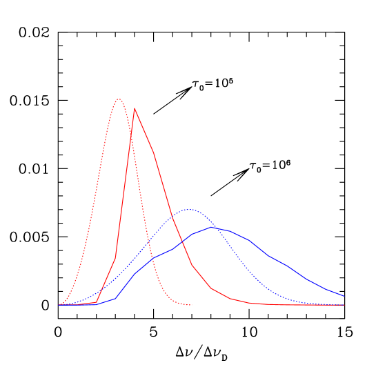
Figure 4: Our emergent profiles (solid lines) are compared with Neufeld’s analytic solution (dotted lines). $x$ axis is a frequency in units of the thermal width, and the total flux of the line is normalized to $1/8\pi$ in accordance with Neufeld’s normalization. The profiles are symmertic about the origin, $\Delta\nu/\Delta\nu_{D}=0$.

Neufeld (1990) derived an analytic solution, for $(a\tau_{0})^{1/3}\gg 1$. According to Unno (1955), Harrington (1973), and Neufeld (1990), for the cases of dust-free media, the Ly$\alpha$ line transfer equation is given by

$${\partial^{2}J\over\partial\tau^{2}}+{\partial^{2}J\over\partial\sigma^{2}}=-3\phi(x){E(\tau,x)\over 4\pi},$$ (19)

where

$$\sigma=\left({2\over 3}\right)^{1/2}\int_{0}^{x}{dx^{\prime}\over\phi(x^{\prime})},$$ (20)

and $\phi(x)$ is the normalized Voigt function given by

$$\phi(x)={1\over\sqrt{\pi}}H(x,a).$$ (21)

Here the boundary conditions are

$$J(\tau,\pm\infty)=0$$ (22)

$$J(\pm\tau_{0},x)=\pm 2H(\pm\tau,x)=\mp{2\over 3\phi(x)}\left({\partial J\over\partial\tau}\right)_{\pm\tau_{0}}.$$ (23)

Since the source function $E(\tau,x)$ in the right hand side of Eq. (19) is very sharply peaked, we can apply the Green function method to the problem. With an approximaton

$$\phi(x)\simeq a/\pi x^{2}$$ (24)

and an application of the Sturm-Lioville theory, Neufeld (1990) derived a solution for the case of a mid-plane source,

$$J(\pm\tau_{0},x)={\sqrt{6}\over 24}{x^{2}\over a\tau_{0}}{1\over\cosh[(\pi^{4}/54)^{1/2}(|x^{3}-x_{i}^{3}|/a\tau_{0})]}.$$ (25)

We perform Monte Carlo calculations for a monochromatic source with $x_{i}=0$, and compare the result with Eq.(24). Fig. 4 shows our results for $\tau=10^{5}$ and $\tau_{0}=10^{6}$. The solid lines are the results of Monte Carlo calculation, and the dotted lines are those obtained by Neufeld. The shapes of the profiles agree with each other, and we emphasize that our Monte Carlo code is written to incorporate all the quantum mechanics associated with both resonant and non-resonant Ly$\alpha$ scattering.

The figure shows an overall disagreement: the Monte Carlo solution appears to be translated from the Neufeld’s solution by an amount of $x\simeq 3$, which corresponds to the frequency shift where the wing scattering becomes important and the profile function $\phi(x)$ can be nicely approximated by Eq. (24). In fact, in the cases of dust free media, no loss of Ly$\alpha$ line photons is permitted, which guarantees the flux conservation. The profile function $\phi(x)$ can not be approximated by Eq.(23) at $x\leq 3$, and therefore, Neufeld’s calculation underestimates the amount of core photons that are removed and ultimately redistributed to the wing regimes, which reduces the amount of diffusively trasferred wing photons.

3.3 Survival Fraction for Dusty Media

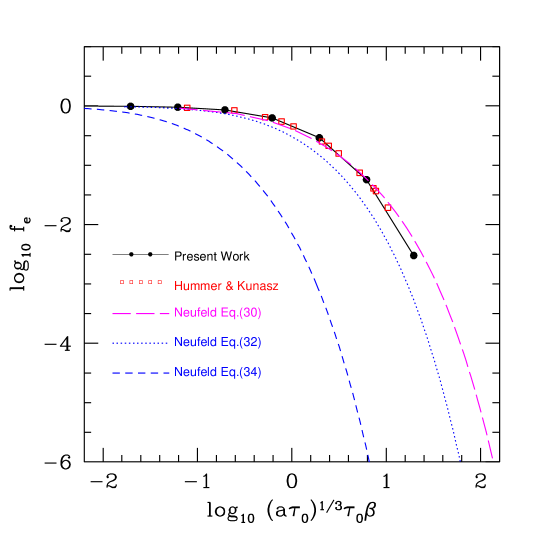
Figure 5: Survival fraction of photons in our Monte Carlo calculations for dusty media of $\tau_{0}=10^{6}$ is compared with previous works. Long dashed line stands for the case of a variable effective frequency, and dotted line for the case of a constant effective frequency. Short dashed line represents Neufeld’s derivation for $Y_{0}$ by considering average scattering number of photons in media with intermediate optical depth.

Neufeld (1990) also provided an analytic solution for the problem of the radiative transfer in a dusty medium. Here we will concentrate on the continuum absorption case. Harrington (1973) and Neufeld (1990) formulated this problem by

$${\partial^{2}J\over\partial\tau^{2}}+{\partial^{2}J\over\partial\sigma^{2}}=-3[\phi(x)+\beta_{t}(x)]\left[{E(\tau,x)\over 4\pi}-\beta(x)J\right],$$ (26)

where

$$\sigma=\left({2\over 3}\right)^{1/2}\int_{0}^{x}{dx^{\prime}\over\phi(x^{\prime})+\beta_{t}(x^{{}^{\prime}})}.$$ (27)

We assume that the total dust opacity $\beta_{t}(x)\approx 0$ becasue $\phi(x)\gg\beta_{t}$. Here, $\beta$ is an absorptive part of dust opacity per atomic hydrogen, which is given by

$$\beta=1.0\times 10^{-8}T_{g4}^{1/2}{n_{H}\over n_{HI}}\xi_{d}.$$ (28)

Here

$$\xi_{d}=(1-A){\tau_{d}\over N_{HI}}/\left[(1-A){\tau_{d}\over N_{HI}}\right]_{G},$$ (29)

where A is albedo and the subscript $G$ represents the Galactic value. A dust opacity per a hydrogen atom is given by

$${\tau_{d}\over N_{HI}}=f_{d}(\sigma_{sca}+\sigma_{abs}),$$ (30)

where $\tau_{d}$ is dust optical depth, $f_{d}$ is dust-to-gas ratio, $\sigma_{sca}$ and $\sigma_{abs}$ are the scattering and the absorption cross sections, respectively. According to Draine and Lee (1984), the mean value of the dust optical depth for Our Galaxy is given by $\tau_{d}/N_{HI}=1.6\times 10^{-21}$ at $\lambda_{0}=1216\AA$.

In our Monte Carlo code, we give $\tau_{d}$, $A$, as well as $N_{HI}$ or $\tau_{0}$. Therefore we can compare these two kinds of calculations. Neufeld also gave solutions for two kinds of approximation: (1) variable effective scattering frequency, (2) constant effective scattering frequency. In the former approximation, the survival fraction of photons is given by

$$f_{e}=\left[1+\sum_{k=1}^{\infty}\left({y_{0}^{2k}\over k!}{1\over 3\cdot 7\cdot 11\cdot\cdot\cdot\cdot(4k-1)}\right)\right]^{-1},$$ (31)

where $y_{0}\equiv{3\over 2}({16\over\pi})^{1/6}a^{1/6}\beta^{1/2}|\tau_{0}|^{2/3}$.

In the latter approximation, the total fraction of photons which escape the slab is given by

$$f_{e}={1\over\cosh(Y_{0})},$$ (32)

where

$$Y_{0}=\left[{3(a\tau_{0})^{1/3}\beta\tau_{0}\over\pi\zeta^{2}}\right]^{1/2},$$ (33)

and $\zeta$ is determined to be $\zeta=0.525$ by fitting the results of Hummer and Kunasz (1980) to the following relation between peak frequency ($x_{s}$) and the $a\tau_{0}$,

$$x_{s}=\zeta(a\tau_{0})^{1/3}.$$ (34)

The other way of determining $Y_{0}$ is provided by Neufeld (see Eq. 4.35 in his paper), who considered the mean scattering length in the result of Hummer and Kunasz (1980). The consideration leads to an survival fraction $1/\cosh(Y_{0})$ with

$$Y_{0}=\left(31.8\beta\tau_{0}\right)^{1/2}.$$ (35)

He argued that this relationship may be applicable even in the range of intermediate optical depth, $10^{3}<\tau_{0}<10^{3}/a$.

In Fig. 5 we show the main result on the survival fraction of Ly$\alpha$ photons in a dusty medium with $\tau_{0}=10^{6}$ and $T=10^{4}{\rm\ K}$. Our results are in good agreement with Neufeld’s approximate solutions and those of Hummer and Kunasz. Our results are also consistent with Neufeld’s approximation solution for the approximation of a constant effective frequency.

On the other hand, although Neufeld noted that Eq.(34) above is valid even in intermediate optical depths, according to our results, this statement is not true.

4 Discussion

In this paper we described the Ly$\alpha$ line transfer in an optically thick, dusty, and static medium. We took accurate atomic physical considerations in the Monte Carlo code, and examined the effect of dusts on Ly$\alpha$ line formation in optically thick media.

For dust free media we confirmed the line transfer mechanism, in which a number of longest flights occur. We emphasize that photons experience a series of wing scatterings at the moment of escape, at which stage significant polarization can be developed. We also confirmed that line profiles from our Monte Carlo calculations agree well with the analytic solution derived by Neufeld (1990).

For dusty media, we calculated the survival fraction of photons for $\tau_{0}=10^{6}$ and $T=10^{4}K$, and found that our results are in good agreement with those obtained by Hummer and Kunasz (1980) and with those of Neufeld’s approximation solution.

The computational speed is limited for extremely thick media with $a\tau_{0}>10^{3}$. This difficulty can be overcome by considering only wing scatterings (Adams 1972). Hence, we are now writing a Monte Carlo code similar to that of Adams. Also we will investigate effects of following various deviations from our simplified configuration: the initial line width, the bulk motion of scatterers, the geometrical shape of scattering media, the degree of homogeneity of the dusts, and the distribution form of photon sources.

One of main goals of our research is to develop a tool to estimate the dust abundance in accordance with the usual method using the Balmer decrement (see Osterbrock 1989) and the slope of UV continuum (Fall & Pei 1989). This may help us correct properly the dust extinction of emission lines in starburst galaxies. Especially this will enable us to estimate the star formation rate of those galaxies which are located near or far.

The other ramification is the formation of the damped Ly$\alpha$ absorption (DLA) in many quasar spectra. The dust contents in DLA galaxies may deform the absorption profile. This may spoil the usual Voigt profile fitting procedure, and subsequent derivation of physical values can be erroneous.

References

- (1) Adams, T. 1972, ApJ, 174, 439
- (2) Draine, B. T. & Lee, H. M. 1984, ApJ, 285, 89
- (3) Fall, S. M. & Pei, Y. 1989, ApJ, 337, 7
- (4) Gould A. & Weinberg D. H. 1996, ApJ, 468, 462
- (5) Gray D. F. 1992, in The Observation and Analysis of Stellar Photospheres 2nd ed. Cambridge Press, New York
- (6) Harrington, J. P. 1973, MNRAS, 162, 43
- (7) Hummer, D. G. & Kunasz, P. B. 1980, ApJ, 236, 609
- (8) Kunth, D., Mas-Hesse, J. M., Terlevich, E., Terlevich, R., Lequeux, J., & Fall, S. M. 1998, AA, 334, 11
- (9) Leitherer, C. et al. 1999, ApJS, 123, 3
- (10) Lee, H.-W. & Ahn, S.-H 1998, ApJ, 504, L61
- (11) Lee, H.-W. & Blandford, R. D. 1997, MNRAS, 288, 19
- (12) Meurer, G. R., Heckman, T. M., Calzetti, D. 1999, ApJ, 521, 6 4
- (13) Miralda-Escude, J. & Rees, M. J. 1998, ApJ, 497, 21
- (14) Neufeld, D. A. 1990, ApJ, 350, 216
- (15) Osterbrock, D. E. 1962, ApJ, 135, 195
- (16) Osterbrock, D. E. 1989, Astrophysics of Gaseous Nebulae and Active Galactic Nuclei, University Science Books, California
- (17) Ogle, P. M. 1999 ApJS, 125, 1
- (18) Phillips, K. C. & Mészáros, P. 1986, ApJ, 310, 284
- (19) Press W. H., Flannery B. P., Teukolsky S. A., & Vetterling W. T. 1989, Numerical Recipes, Cambridge Press, New York
- (20) Rybicki G. B & Lightman A. P. 1979, Radiative Processes in As trophysics, John Wiley & Sons, New York
- (21) Stenflo, J. O. 1980, A&A, 1984, 68
- (22) Unno, W. 1955, PASJ, 7, 81