Theoretical and Experimental Topics on Ultra High Energy Cosmic Rays

Abstract

Since their first observation in 1962, the existence of Ultra High Energy Cosmic Rays (UHECR) remains a mystery in modern astrophysics. Those cosmic rays, with energies well above 50 EeV ($50\times 10^{18}$eV), can hardly be accelerated, even in the most active parts of our universe such as FR-II radio galaxies or AGNs, nor can they travel on distances larger than 100 Mpc. In the following some of the production and acceleration models for UHECR are reviewed and some of the transport issues are exposed. Finally the detection and identification on Earth of those “cosmic bullets” are presented.

1 Introduction

This lecture is mainly concerned with the problems of the existence and observation of cosmic rays whose energies are above $5\times 10^{19}$ eV. Such cosmic rays - for which we shall use the term “ultra high energy cosmic rays” or UHECR - are exceptional for the following reasons:

• They are above the Greisen-Zatsepin-Kuzmin (GZK) cutoff[1] which corresponds to the proton energy threshold for pion photo-production on the cosmic microwave background (CMB). Similar cutoffs exist at lower energies for gammas interacting with background photons (CMB, infra-red or radio waves). Consequently, and except for neutrinos, if the UHECR observed on Earth are due to the known stable particles, they must be produced in our vicinity. At the GZK cutoff, the “visible” universe shrinks suddenly to a sphere of a few tens of megaparsecs (Mpc).

• There are very few conventional astrophysical sources able to accelerate particles at energies exceeding 10²⁰ eV, those of the most energetic UHECR that have been observed up to now.

• At such energies and in most field models, the bending effect of the galactic and extragalactic magnetic fields are quite weak. Thus, even for charged particles, the reconstructed incident direction points toward the source within a few degrees. Unlike with lower energy cosmic rays one can do point-source-search astronomy with UHECR.

The widely shared excitement about the UHECR comes from the above considerations and from the study of the scarce data available. If the sources are astrophysical macroscopic objects, they must be visible through some counterpart that optical or radio-astronomy should detect. But there are no remarkable object visible in the directions pointed at by UHECR. There is even no convincing evidence that one can find any correlation between the incoming directions and the inhomogeneous distribution of matter in our vicinity.

In the following, we shall develop in detail the facts and arguments briefly mentioned in this introduction. In section 2 we present the candidate source characteristics and we discuss the transport problems. Section 3 is devoted to cosmic ray interactions in the atmosphere and section 4 to detection techniques. Finally section 5 describes some of the available experimental results.

To avoid repetitive use of large powers of ten, the energy units in the following will mostly be in zetta-electron-volts (ZeV, 10²¹ eV) and exa-electron-volts (EeV, i.e. 10¹⁸ eV).

2 Production and Transport of UHECR

Today’s understanding of the phenomena responsible for the production of UHECR, i.e. the transfer of macroscopic amounts of energy to microscopic particles, is still limited. One distinguishes two classes of processes: the so called “Top-Down” and “Bottom-Up” scenarios. In the former, the cosmic ray is one of the stable decay products of a super-massive particle. Such particles with masses exceeding 1 ZeV can either be meta-stable relics of some primordial field or highly unstable particles produced by the radiation, interaction or collapse of topological defects. Those processes are reviewed in Section 2.3

In the second scenario discussed in section 2.2 the energy is transferred to the cosmic rays through their interaction with electromagnetic fields. This classical approach does not require new physics as opposed to the “Top-Down” mechanism, but does not exclude it either since, in some models, the accelerated particle - the cosmic ray - is itself “exotic”.

Once accelerated the cosmic rays must propagate from their source to the observer. At energies above 10 EeV and except for neutrinos, the Universe is not transparent to ordinary stable particles on scales much larger than about 10 Mpc. Regardless of their nature, cosmic rays lose energy in their interaction with the various photon backgrounds, dominantly the copious Cosmic Microwave Background (CMB) but also the Infra-Red/Optical (IR/O) and the Radio backgrounds. The GZK cutoff puts severe constraints on the distance that a cosmic ray can travel before losing most of its energy or being absorbed. The absence of prominent visible astrophysical objects in the direction of the observed highest energy cosmic rays together with this distance cutoff adds even more constraints on the “classical” Bottom-Up picture.

It is beyond the scope of this lecture to describe all the scenarios - they are far too numerous - proposed for the production of the UHECR. Let us simply agree on the fact that the profusion of models shows that none of them is totally satisfactory and that data are not very constraining. Consequently we will try to present, from an experimentalist’s point of view, the main features of the various categories of models. We will also try to focus on the possible experimental constraints, if they exist, or on the problems related to the UHECR and which remain unsolved. For a more detailed review we urge the reader to consult the excellent report by P.Bhattacharjee and G.Sigl[2] and the references therein. Extensive use of this report is made in some of the following sections where we avoided repeated reference to it.

At first sight, it would seem natural to discuss potential sources and acceleration mechanisms before the description of the cosmic ray transportation to Earth. However, and because the attenuation or interaction lengths are relatively short and strongly energy dependent in the range of interest, the observed spectra do not only depend on the nature of the sources but also on their distribution. In addition, the GZK cutoff puts important constraints which we prefer to discuss before describing the possible nature of the sources themselves.

2.1 Propagation

We will focus here on the propagation of atomic nuclei (in particular protons) and photons. Electrons are not considered as potential UHECR because they radiate most of their energy while crossing the cosmic magnetic fields. Among the known stable particles, and within the framework of the Standard Model, those are the only possible candidates for UHECR. As mentioned in Section 5.2, the actual data effectively favor a hadronic composition.

Neutrinos and the lightest super-symmetric particles (LSP) should deserve special attention as they may travel through space unaffected even on large distances. However, for neutrinos the interaction should occur uniformly in atmospheric depth, a feature which is not reproduced by the current data. While neutrinos may very well be one of the components of the high energy end of the cosmic ray spectrum and prove to be an unambiguous signature of the new physics underlying the production mechanisms (see below) they do not seem to dominate the observations at least up to energies of a few 10²⁰ eV.

The LSP are expected to have smaller interaction cross sections with photons and a higher threshold for pion photo-production due to their higher mass (see Eq. (1) below). Therefore they may travel unaffected by the CMB on distances 10 to 30 times larger than nucleons. However in usual models the LSP is neutral and cannot be accelerated in a Bottom-Up scenario and must be produced as a secondary of an accelerated charged particle (e.g. protons). This accelerated particle must reach energies at least one order of magnitude larger than the detected energy (order of ZeV) and will produce photons. The acceleration site should therefore be detectable as a very powerful gamma ray source in the GeV range. In a Top-Down scenario including Super-Symmetry, the problem of propagation is of somewhat lesser importance as the decaying super-massive particles may be distributed on cosmological or on nearby scales and are, in any case, invisible (see Section 2.3). Finally let us stress that the analysis of the UHECR shower shape limits the mass of the cosmic ray to about 50 GeV,[3] an additional constraint for the LSP candidate.

2.1.1 Protons and Nuclei: The GZK cutoff

The Greisen-Zatsepin-Kuzmin (GZK) cutoff (see Section 1) threshold for collisions between the cosmic microwave background (CMB) and protons (pion photo-production) can be expressed in the CMB “rest” frame as

$$E_{th}\simeq\frac{E_{\gamma}^{lab}m_{p}}{2\epsilon}\sim\frac{7\times 10^{16}}{\epsilon}eV$$ (1)

where $\epsilon$ is the CMB photon energy, $E_{\gamma}^{lab}=m_{\pi}^{2}/2m_{p}+m_{\pi}$ is the photon threshold for a proton at rest and $E_{th}$ the proton threshold in the CMB frame, all in electron-volts. For an energetic CMB photon with $\epsilon=$ 10^-3 eV, $E_{th}$ is $7\times$10¹⁹ eV which is where one expects the GZK cutoff to start.

The interaction length for this process can be estimated from the pion photo-production cross section (taken beyond the $\Delta$ resonance production) and the CMB photon density:

$$L=(\sigma\rho)^{-1}\simeq 1.8\times 10^{25}\,\mbox{cm}\simeq 6\,\mbox{Mpc}$$

for $\rho=410\,\mbox{cm}^{-3}$ and $\sigma=135~{}\mu$barns.

file=./adrf25.eps, width = 8cm

Figure 1: Energy of a proton as a function of the propagation distance through the 2.7K cosmic background radiation for various initial energies.

The energy loss of protons of various initial energies as a function of the propagation distance is shown in Figure 1. Above 100 Mpc the observed energy is below 10²⁰ eV regardless of its initial value. One should point out that this reduction is not the consequence of a single catastrophic process but of many collisions (more than 10) each of which reduces the incident energy by 10 to 20%. Therefore the probability to travel without losses is negligible.

A proton may also produce $e^{+}e^{-}$ pairs on the CMB at a much lower threshold (around $5\times$10¹⁷ eV) but the cross section is orders of magnitude smaller and together with a much smaller energy loss per interaction the overall attenuation length stays around 1 Gpc.

For nuclei, the situation is in general more difficult. They undergo photo-disintegration in the CMB and infrared radiations losing on average 3 to 4 nucleons per Mpc when their energy exceeds 2$\times$10¹⁹ eV to 2$\times$10²⁰ eV depending on the IR background density value. The IR background is much less well known than the CMB and the attenuation length (see Figure 2) derived for nuclei must be taken with precaution.

file=./adrf24.eps, width = 8cm

Figure 2: Attenuation length of photons, protons and iron in various background radiation as a function of energy. The dot-dashed line represents the absolute upper limit on the distance a particle can travel toward Earth, regardless of its initial energy.

2.1.2 Electrons and Photons: Electromagnetic Cascades

Top-Down production mechanisms predict that, at the source, photons (and neutrinos) dominate over ordinary hadrons by about a factor of ten. An observed dominance of gammas in the supra-GZK range would then be an almost inescapable signature of a super-heavy particle decay. Photons are also secondaries of more ordinary processes such as pion photo-production; their propagation is thus worth studying. Unlike photons, electrons and positrons cannot constitute the primary CR as the radiation energy losses they undergo forbid them to reach the highest energies by many orders of magnitude.

High energy photons traveling through the Universe produce $e^{+}e^{-}$ pairs when colliding with the Infra-Red/Optical (IR/O), CMB or Universal Radio Background (URB) photons. As can be seen on Figure 2 the attenuation length gets below 100 Mpc for photon energies between $3\times$10¹² eV and 10²² eV. In this energy range, nearly 10 orders of magnitude, the Universe is opaque to photons on cosmological scales.

Once the photon converted, the $e^{+}e^{-}$ pair will in turn produce photons mostly via Inverse Compton Scattering (ICS) (the case of synchrotron radiation, usually non dominant, will be treated in the next section). At our energies, those two dominant processes are responsible for the production of electromagnetic (EM) cascades.

Far above the pair production threshold ($s\gg 4m_{e}^{2}$, where $\sqrt{s}$ is the CM energy) the ICS ($\sigma_{\mbox{ICS}}$) and the pair production ($\sigma_{\mbox{pp}}$) cross sections are related by :

$$\sigma_{\mbox{pp}}\approx 2\sigma_{\mbox{ICS}}=\frac{3}{2}\sigma_{T}\frac{m_{e}^{2}}{s}\log\left(\frac{s}{2m_{e}^{2}}\right)$$

where $m_{e}$ is the electron mass and $\sigma_{T}=8\pi\alpha^{2}/3m_{e}^{2}=665$ mbarn the Thomson cross section for photon elastic scattering on an electron at rest. The $1/s$ dependence implies that far from the pair threshold the EM cascade develops slowly as it is the case when the initial photon energy is above 10²² eV.

At the pair production threshold ($s\sim 4m_{e}^{2}$), the pair cross section reaches $\sim 170$ mbarn and $\sigma_{\mbox{ICS}}$ is nearly equal to the Thomson cross section. The EM cascades develop very rapidly. From Figure  2 one sees that at the pair production threshold on the CMB photons ($2\times$10¹⁴ eV) conversion occurs on distances of about 10 kpc (a thousand times smaller than for protons at GZK energies) while subsequent ICS of electrons on the CMB in the Thomson regime will occur on even smaller scales (1 kpc).

As a consequence, all photons of high energy (but below 10²² eV) will produce, through successive collisions on the various photon backgrounds (URB, CMB, IR/O), lower and lower energy cascades and pile up in the form of a diffuse photon background below 10¹² eV with a typical power law spectrum of index $\alpha=1.5$. This is a very important fact as measurements of the diffuse gamma ray background in the $10^{7}$-10¹¹ eV range done for example by EGRET[4] will impose limits on the photon production fluxes of Top-Down mechanisms and consequently on the abundance of topological defects or relic super-heavy particles.

2.1.3 Charged Particles: Magnetic Fields

The effect of magnetic fields (galactic or extragalactic) on the deflection of charged particles will be reviewed in Section 5.3.1. Here we will present some of the effects of the fields on EM cascade production.

Electrons and positrons produced through EM cascades lose energy via synchrotron radiation at a rate given by:

$$-\frac{dE}{dt}=\frac{4\alpha^{2}}{3m_{e}^{2}}<B^{2}>\left(\frac{E}{m_{e}}\right)^{2},$$

where we assume a random field $B$ isotropically distributed with respect to the electron direction.

At high enough energy, i.e.

$$E\sim\left(\frac{B}{10^{-9}\,\mbox{G}}\right)^{-1}10^{19}\,\mbox{eV}$$

this process will dominate over ICS on URB or CMB photons. In a nanoGauss field and at 10¹⁹ eV the loss is about $3\times$10¹⁸ eV over 100 kpc. The above threshold is not very strict as it depends on the URB density which is not a very well known quantity. The emitted gammas have a typical energy given by[2]

$$E_{\mbox{synch}}=6.3\times 10^{11}\left(\frac{E}{10^{19}\,\mbox{eV}}\right)\left(\frac{B}{10^{-9}\,\mbox{G}}\right)\mbox{eV}.$$

Again low energy photon flux measurements will put constraints on the extragalactic fields and/or on the initial photon flux.

Above threshold, the synchrotron radiation will damp the electron-positron pair energy extremely quickly. At 100 EeV in a $10^{-9}$ G magnetic field the attenuation length is of the order of 20 kpc. If one observes gammas above 10²⁰ eV they could not be high energy secondaries (e.g. from ICS) of an even higher energy photon converted into a pair. They must instead be primary ones. Consequently, their flux $j_{\gamma}(E)$ per unit area and unit solid angle at a given energy is directly related to the source distribution without any transport nor cosmological effects in between :

$$j_{\gamma}(E)\sim\frac{1}{4\pi}l_{\gamma}(E)\phi(E)$$

where $\phi(E)$ is the source density per unit time and energy interval and $l_{\gamma}(E)$ is the photon interaction length.

Of course quantitative predictions of such effects is pending definite measurements of the galactic and extragalactic magnetic fields. Although the magnetic fields of the galactic disc are now believed to be fairly well known this is not the case of the ones in the halo or extragalactic media. As mentioned in Section 5.3.1, several authors advocate our bad knowledge of those fields in explaining the puzzling observational data and question both the typical value of $10^{-9}$ G and the coherence length of 1 Mpc usually assumed for the extragalactic fields.[5]

2.2 Conventional acceleration: Bottom-Up scenarios

One essentially distinguishes two types of acceleration mechanisms :

• Direct, one-shot acceleration by very high electric fields. This occurs in or near very compact objects such as highly magnetized neutron stars or the accretion disks of black holes. However, this type of mechanism does not naturally provide a power-law spectrum.

• Diffusive, stochastic shock acceleration in magnetized plasma clouds which generally occurs in all systems where shock waves are present such as supernova remnants or radio galaxy hot spots. This statistical acceleration is known as the Fermi mechanism of first (or second) order, depending on whether the energy gain is proportional to the first (or second) power of $\beta$, the shock velocity.

Extensive reviews of acceleration mechanisms exist in the literature, e.g. on acceleration by neutron stars,[6] shock acceleration and propagation,[7] non relativistic shocks,[8] and relativistic shocks.[9]

Hillas has shown[10] that irrespective of the details of the acceleration mechanisms, the maximum energy of a particle of charge $Ze$ within a given site of size $R$ is:

$$E_{\mbox{max}}\approx\beta Z\left(\frac{B}{1\,\mu\mbox{G}}\right)\left(\frac{R}{1\,\mbox{kpc}}\right)10^{18}~{}\mbox{eV}$$ (2)

where $B$ is the magnetic field inside the acceleration volume and $\beta$ the velocity of the shock wave or the efficiency of the acceleration mechanism. This condition essentially states that the Larmor radius of the accelerated particle must be smaller than the size of the acceleration region, and is nicely represented in the Hillas diagram shown in Figure 3.

file=./Hillas.ps, width = 8cm

Figure 3: Size and magnetic field strength of possible acceleration sites. Objects below the diagonal lines cannot accelerate the corresponding elements (Iron with $\beta=1$ or protons $\beta=1$ and $\beta=1/300$) above 10²⁰ eV.

2.2.1 Candidate sites

Inspecting the Hillas diagram one sees that only a few astrophysical sources satisfy the necessary, but not sufficient, condition given by Eq. (2). Some of them are reviewed e.g. by Biermann.[11] Let us just mention, among the possible candidates, pulsars, Active Galactic Nuclei (AGN), Fanaroff-Riley Class II (FR-II) radio galaxies and Gamma Ray Bursts (GRB).

Pulsars 
From a dimensional analysis, the electric field potential drop in a rotating magnetic pulsar is given by:

$$\Delta\Phi=\frac{B\times R^{2}}{\Delta T}$$ (3)

One obtains $e\Delta\Phi=100$ EeV with $B=10^{9}\,$T, $\Delta T=10^{-3}\,$s and $R=10^{4}\,$m. However the high radiation density in the vicinity of the pulsar will produce $e^{+}e^{-}$ pairs from conversion in the intense magnetic field.[6] These pairs will drift in opposite directions along the field lines and short circuit the potential drop down to values of about 10¹³ eV. Moreover in the above dimensional analysis a perfect geometry is assumed. Actually, a more realistic geometry would introduce an additional factor $R/c\Delta T\sim 0.1$, and further decrease the initial estimate. Finally, as will be described in the next section, synchrotron radiation losses in such compact systems become very important even for protons.

AGN cores and jets 
Blast wave in AGN jets have typical sizes of a few percent of a parsec with magnetic fields of the order of 5 gauss.[12] They could in principle lead to a maximum energy of a few tens of EeV. Similarily for AGN cores with a size of a few $10^{-5}$ pc and a field of order $10^{3}$ G one reaches a few tens of EeV. However those maxima, already marginal, are unlikely to be achieved under realistic conditions. The very high radiation fields in and around the central engine of an AGN will interact with the accelerated protons producing pions and $e^{+}e^{-}$ pairs. Additional energy loss due to synchrotron radiation and Compton processes lead to a maximum energy of about 10¹⁶ eV, much below the initial value.[2] To get around this problem, the acceleration site must be away from the active center and in a region with a lower radiation density such as in the terminal shock sites of the jets: a requirement possibly fulfilled by FR-II radio galaxies.

FR-II radio galaxies 
Radio-loud quasars are characterized by a very powerful central engine ejecting matter along thin extended jets. At the ends of those jets, the so-called hot spots, the relativistic shock wave is believed to be able to accelerate particles up to ZeV energies. This estimate depends strongly on the value assumed for the spots’ local magnetic field, a very uncertain parameter. Nevertheless FR-II galaxies seem the best potential astrophysical source of UHECR.[11] Unfortunately, no nearby (less than 100 Mpc) object of this type is visible in the direction of the observed highest energy events. The closest FR-II source, actually in the direction of the Fly’s Eye event at 320 EeV, is at about 2.5 Gpc, way beyond the GZK distance cuts for nuclei, protons or photons.

Gamma Ray Burst 
Gamma ray bursters (GRB) are intense source of gamma rays of a few milliseconds with gamma energies ranging from about 1 KeV to a few GeV. Several hundreds have been observed by satellites. The most favored GRB emision model is the “expanding fireball model” where one assumes that a large fireball, as it expends, becomes optically thin hence emitting a sudden burst of gamma rays. The engine (the power source) of such a fireball remains unknown whilst the explanation of the non thermal spectra observed needs some additionnal modeling (such as internal shocks in the expanding fireball).

The observation of afterglow (low energy gamma ray emission of the heated gas in which the fireball expanded) allowed to measure the red shift of the GRBs from which one confirmed their cosmological origin (and a support for the fireball model). Under certain conditions, GRB can be shown to accelerate protons up to 10²⁰ eV therefore making them a good candidate site for UHECR production. However in such a framework the UHECR spectrum should clearly show the GZK cut-off while above 10²⁰ eV the distribution of arrival directions should be strongly anisotropic. Although more data is needed the 20 events already observed above 10²⁰ eV do not seem to confirm this hypothesis. In addition, the detection of high energy neutrinos (10¹⁴ eV and eventually 10¹⁸ eV depending on the GRB environment) in coincidence with the gamma burst would be a strong evidence for this model[13].

2.2.2 Additional constraints

In addition to the constraint given by Eq. (2), candidate sites must also satisfy two additional conditions.

• The acceleration must occur on a reasonable time scale, e.g. the size of the acceleration region must be less than the interaction length of the accelerated particle. This is a relatively weak constraint since all the objects in the Hillas diagram have a size below 1 Mpc. However, in shock acceleration mechanisms the rate of energy loss on the CMB must be less than the rate of energy gain:

  $$-\frac{dE_{\mbox{loss}}}{dt}\propto\mbox{const}\times E<\frac{dE_{\mbox{gain}}}{dt}$$ (4)

• The acceleration region must be large enough so that synchrotron losses are negligible compared to the energy given by Eq. (2). For shock acceleration the radiated synchrotron power must be below the rate of energy gain:

  $$-\frac{dE_{\mbox{sync}}}{dt}\propto\frac{E^{4}}{R^{2}}\propto B^{2}~{}E^{2}$$ (5)

file=./adrf23.eps, width = 8.5cm

Figure 4: Magnetic field strength and shock velocity of possible sites. GC refers to Galactic Cluster (accretion shocks), IGM to Inter Galactic Medium, RGL to Radio Galaxy Lobes and RGH to Radio Galaxy Hot Spots (a subclass of RGL).

Using, as the characteristic acceleration time, $T_{A}=R/\beta$ (where $\beta$ is the shock velocity) one finds a characteristic gain rate of :

$$\frac{dE_{\mbox{gain}}}{dt}\approx\frac{E_{\mbox{max}}}{T_{A}}\propto\beta^{2}~{}B.$$ (6)

For a given $E_{\mbox{max}}$ (e.g. 100 EeV), these two constraints define two lines in the $\log{B}$, $\log{\beta}$ plane above and below which particles cannot be accelerated at the required energy. As can be seen on Figure 4 the only remaining candidates are the radio galaxy hot spots (RGH).

To conclude on the bottom-up scenario, let us mention a recent analysis from Farrar and Biermann.[14] They have shown that, on cosmological scales, the correlation between the arrival direction of the five highest energy events and Compact Quasi Stellar Objects (CQSO’s) which include radio-loud galaxies is unlikely to be accidental. However, only a new type of neutral particle could travel on distances over 1 Gpc without losing its energy on the CMB nor being deflected by extragalactic magnetic fields. More data at very high energy are needed to validate this result which would sign the existence of a new particle physics phenomenon.

2.3 “Exotic” sources: Top-Down scenario

One way to overcome the many problems related to the acceleration of UHECR, their flux, the visibility of their sources and so on, is to introduce a new unstable or meta-stable super-massive particle, currently called the $X$-particle. The decay of the $X$-particle produces, among other things, quarks and leptons. The quarks hadronize, producing jets of hadrons which, together with the decay products of the unstable leptons, result in a large cascade of energetic photons, neutrinos and light leptons with a small fraction of protons and neutrons, part of which become the UHECR.

For this scenario to be observable three conditions must be met:

• The decay must have occurred recently since the decay products must have traveled less than about 100 Mpc because of the attenuation processes discussed above.

• The mass of this new particle must be well above the observed highest energy (100 EeV range), a hypothesis well satisfied by Grand Unification Theories (GUT) whose scale is around $10^{24}$-10²⁵ eV.

• The ratio of the volume density of this particle to its decay time must be compatible with the observed flux of UHECR.

The $X$-particles may be produced by way of two distinct mechanisms:

• Radiation, interaction or collapse of Topological Defects (TD), producing $X$-particles that decay instantly. In those models the TD are leftovers from the GUT symmetry breaking phase transition in the very early universe. Quantitative predictions of the TD density that survives a possible inflationary phase rely on a large number of theoretical hypotheses. Therefore they cannot be taken as face value, although the experimental observation of large differences could certainly be interpreted as the signature of new effects.

• Super-massive metastable relic particles from some primordial quantum field, produced after the now commonly accepted inflationary stage of our Universe. Howerver the ratio of their lifetime to the age of the universe requires a fine tuning ($10^{-11}$) with their relative abundance as is discussed in section2.3.3. It is worth noting that in some of those scenarios the relic particles may also act as non-thermal Dark Matter.

In the first case the $X$-particles instantly decay and the flux of UHECR is related to their production rate given by the density of TD and their radiation, collapse or interaction rate, while in the second case the flux is driven by the ratio of the density of the relics over their lifetime. In the following the terms “production or decay rate” will refer to these two situations. Before discussing the exact nature of the $X$-particles we shall briefly review the main characteristics of the decay chain and the expected flux of the energetic outgoing particles.

2.3.1 $X$decay and secondary fluxes

At GUT energies and if they exist, squark and sleptons are believed to behave like their corresponding super-symmetric partners so that the gross characteristics of the cascade may be inferred from the known evolution of the quarks and leptons. Of course the internal mechanisms of the decay and the detailed dynamics of the first secondaries do depend on the exact nature of the particles but the bulk flow of outgoing particles is most certainly independent of such details.[2]

A common picture for the hadronisation of the decay products follows three steps. At the high energy end, the perturbative QCD-inspired recipes provide a good framework for the description of the hard processes driving the dynamics of the parton cascade. At a cutoff energy of about 1 GeV soft processes become dominant and partons are glued together to form color singlets which will in turn decay into known hadrons. The LUND[15] string fragmentation model provides a description for the second and last phases while a model like the Local Parton-Hadron Duality directly relates the parton density in the parton cascade to the final hadron density.[16] Nevertheless and despite the fact that up to 40% of the initial energy may turn into LSP, the cascade produces a rather hard  hadron spectrum adequately described by:

$$\frac{dN_{h}}{dE}\propto E^{-\alpha}\mbox{~{}~{}with~{}~{}}1<\alpha<2$$

in the range $E/m_{X}\ll 1$, where $m_{X}$ is the $X$-particle mass. At the high energy end a cutoff occurs at a value depending on the $X$-particle mass and on the eventual existence of new physics such as Super Symmetry (SUSY), which would displace the maximum of the hadron spectrum to a lower energy (see Figure 5).

file=./Sigl23.eps, width = 8cm

Figure 5: Fragmentation function in the Modified Leading Log Approximation for a total jet energy of $5\times$10²⁴ eV with SUSY (thick solid line peaking at $10^{12}$GeV) and without SUSY (thin solid Line) as calculated by Bhattacharjee and Sigl. Other lines are Hill’s formula (dashed) and an approximated expression (dotted). Note that around 10²⁰ eV, our region of interest, the fluxes are not too widely different.

Indeed, Super Symmetry is not the only candidate theory for new physics beyond the standard model, although the only known acceptable one. Other (yet unknown) models may appear as possible alternatives in the future. However, in all cases, secondaries from Top-Down mechanisms should manifest themselves as a change of slope in the UHECR spectrum, above 10 EeV and over a range which will reflect the (new) physics at play.

In all conceivable Top-Down scenarios, photons and neutrinos dominate at the end of the hadronic cascade. This is the important distinction from the conventional acceleration mechanisms. The spectra of photons and neutrinos can be derived from the charged and neutral pion densities in the jets as:

$$\Phi_{\gamma}^{\pi^{0}}(E,t)\simeq 2\int_{E}^{E_{\mbox{jet}}}\Phi_{\pi^{0}}(\varepsilon,t)d\varepsilon/\varepsilon$$

$$\Phi_{\nu}^{\pi^{\pm}}(E,t)\simeq 2.34\int_{2.34E}^{E_{\mbox{jet}}}\Phi_{\pi^{\pm}}(\varepsilon,t)d\varepsilon/\varepsilon$$

where $E_{\mbox{jet}}$ is the total energy of the jet (or equivalently the initial parton energy). Since $\Phi_{\pi^{\pm}}(\varepsilon,t)\simeq 2\Phi_{\pi^{0}}(\varepsilon,t)$, photons and neutrinos should have very similar spectra. These injection spectra must then be convoluted with the transport phenomena to obtain the corresponding flux on Earth. As was mentioned in Section 2.1.2 the photon transport equation strongly depends on its energy and on the badly known Universal Radio Background and extragalactic magnetic fields.

2.3.2 $X$ production or decay rates: a lower limit

The production or decay rates of the $X$-particles are very model dependent and no firm prediction on the expected flux of UHECR can be made. However, in their review, Bhattacharjee and Sigl evaluate with a simple model the rate needed to explain the observed UHECR fluxes. Assuming that photons dominate at the source and on Earth and that they follow a power law spectrum of index $\alpha$; assuming also that the initial $X$ decay secondaries are quarks and leptons in equal numbers, they calculate a lower limit on the production rate given by (for $\alpha=1.5$):

$$\dot{n}_{X}\geq 10^{-46}\left(\frac{\mbox{10\,Mpc}}{l_{E}(E_{\gamma})}\right)\left(\frac{E^{2}j_{\gamma}(E)}{{\cal F}_{\oplus}}\right)\sqrt{\frac{10^{16}\mbox{GeV}}{m_{X}}}~{}\mbox{cm}^{-3}\mbox{s}^{-1}$$ (7)

Here ${\cal F}_{\oplus}\approx 1$ eV cm^-2s^-1sr^-1 is the observed energy flow of UHECR at 100 EeV and $l_{E}(E_{\gamma})$ the photon attenuation length. Additional normalization factors of order unity have not been reproduced here. In other words, for TD or relics to explain the observed UHECR flux at 100 EeV and assuming an $X$ mass of $10^{16}$ GeV their production or decay rates must be larger than $10^{-46}\mbox{cm}^{-3}\mbox{s}^{-1}$. This is of course only an order of magnitude calculation which may be modified by the decay dynamics and the distribution of the $X$-particles, but can be used as a reasonable scale of the necessary rates.

2.3.3 More about $X$-particles

Topological defects
The very wide variety of topological defect models together with their large number of parameters makes them difficult to review in detail. Many authors have addressed this field. Among them, let us mention Vilenkin and Shellard[17] and Vachaspati[18, 19] for a review on TD formation and interaction, and Bhattacharjee,[20] Bhattacharjee and Sigl[2] and Berezinky, Blasi and Vilenkin[21] for a review on experimental signatures in the framework of the UHECR.

According to the current picture on the evolution of the Universe, several symmetry breaking phase transitions such as $GUT\Longrightarrow H~{}...\Longrightarrow SU(3)\times SU(2)\times U(1)$ occurred during the cooling. For those “spontaneous” symmetry breakings to occur, some scalar field (called the Higgs field) must acquire a non vanishing expectation value in the new vacuum (ground) state. Quanta associated to those fields have energies of the order of the symmetry breaking scale, e.g. $10^{15}-10^{16}$ GeV for the Grand Unification scale. Such values are indeed perfectly in the range of interest for the above mentioned $X$-particles.

During the phase transition process, non causaly connected regions may evolve towards different states - the correlation length is smaller than the horizon - in such a way that at the different domain borders, the Higgs field is forced to keep a vanishing expectation value for topological reasons. Energy is thus trapped at the border called a TD whose properties depend on the topology of the manifold where the Higgs potential reaches its minimum (the vacuum manifold topology).

Possible TDs are classified according to their dimensions: magnetic monopoles (0-dimensional, point-like); cosmic strings (1-dimensional); a sub-variety of the previous which carries current and is superconducting; domain walls (2-dimensional); textures (3-dimensional). Among those, only monopoles and cosmic strings are of interest as possible UHECR sources: textures do not trap energy while domain walls, if they were formed at a scale that could explain EHECR, would over-close the Universe.[22]

In GUT theories, magnetic monopoles always exist because the reduced symmetry group contains at least the electroweak $U_{Y}(1)$ invariance. In fact it is the predicted overabundance of magnetic monopoles in our present universe that led Guth[23] to come up with the now well adopted idea of an inflationary universe. Strings on the other hand are the only defects that can be relevant for structure formation. It is possible, from the scaling property of the string network, to relate the string formation scale $\eta$ to the mass fluctuations in the Universe. Using the large scale mass fluctuation value of $\delta M/M\sim 1$ this gives $\eta\simeq 10^{16}$ GeV and similar conclusions are drawn if one uses the COBE results on CMB anisotropies.[24] It is striking to see that if strings were to play a role in large scale structure formation, hence making the Hot Dark Matter scenario viable,

• the proper energy scale is precisely the grand unification scale of GUT theories,

• this scale also corresponds to the one relevant for UHECR production.

When two strings intercommute, the energy release sometimes leads to the production of small loops that will release more energy when they collapse. These are, among other mechanisms, fundamental dissipation processes that prevent the string network from dominating the energy density in the Universe. For monopoles, it is the annihilation of monopolonia (monopole-antimonopole bound states)[25, 26] that releases energy -although the existence of monopole of the proper energy scale is very questionable as they are either over abundant or washed out by inflation-. In each case part of the released energy is in the form of $X$-particles.

Strings and monopoles come in various forms according to the scale at which TDs are formed and to the vacuum topology. They may even coexist. Nevertheless, the $X$-particle production rate may, on dimensional grounds, be parameterized in a very general way.[27] Introducing the Hubble time $t$, the production rate can be written as:

$$\dot{n}_{X}(t)=\frac{Q_{0}}{m_{X}}\left(\frac{t}{t_{0}}\right)^{-4+p}$$ (8)

where $Q_{0}\equiv\dot{n}_{X}(t_{0})\,m_{X}$ is the energy injection rate at $t=t_{0}$ (the present epoch). The parameter $p$ depends on the exact TD model. In most cases (intercommuting strings, collapsing loops as well as monopolonium annihilation) $p=1$ but superconducting string models can have $p\leq 0$ while decaying vortons  give $p=2$.

One can compare the integrated energy release of Eq. (8) in the form of low energy (10 MeV - 100 GeV) photons resulting from the cascading of the electromagnetic component of the $X$-particle decay with the diffuse extragalactic gamma ray background, $w_{\mbox{em}}\sim 10^{-6}$ eV cm^-3 s^-1, as measured by EGRET. Assuming as in Ref.[21] that half of the energy release goes into the electromagnetic component, one obtains :

$$w_{\mbox{em}}=\frac{Q_{0}}{2}\int_{t_{\mbox{min}}}^{t_{0}}\left(\frac{t}{t_{0}}\right)^{-4+p}\frac{dt}{(1+z)^{4}}.$$ (9)

where $(1+z)=(t_{0}/t)^{2/3}$ in a matter dominated Universe. For $\alpha\equiv p-1/3>0$ evolutionary effects are negligible and Eq. (9) simply leads to

$$w_{\mbox{em}}\simeq\frac{Q_{0}}{2}\frac{t_{0}}{\alpha}$$

or, using the EGRET limit and $t_{0}\simeq 2\times 10^{17}h^{-1}$s, to:

$$\dot{n}_{X}(t_{0})\leq\alpha\frac{10^{-48}h~{}\mbox{cm}^{-3}\mbox{s}^{-1}}{m_{X}/10^{16}\,\mbox{GeV}}$$

a limit hardly compatible with the order of magnitude given by Eq. (7). However, more information about the UHECR fluxes, the diffuse gamma ray background and extragalactic magnetic fields are needed to confirm this.

In the models where $\alpha<0$ evolutionary effects can become important. In fact it is the lower bound of the integral of Eq. (9) that would dominate. Using as a lower bound the decoupling time $t_{\mbox{dec}}/t_{0}\sim 10^{-5}$ one gets:

$$w_{\mbox{em}}\simeq\frac{Q_{0}}{2}\left(\frac{t_{\mbox{dec}}}{t_{0}}\right)^{-\alpha}\frac{t_{0}}{|\alpha|}$$

or,

$$\dot{n}_{X}(t_{0})\leq|\alpha|\frac{10^{-48-5\alpha}\mbox{cm}^{-3}\mbox{s}^{-1}}{m_{X}/10^{16}\,\mbox{GeV}}.$$

which, for $p\leq 0$ is perfectly compatible with Eq. (7). However the large density of gamma rays released in the early Universe impacts on the ⁴He production and on the uniformity of the CMB making this kind of models currently unfavored in the context of UHECR.

Supermassive relics
Supermassive relic particles may be another possible source of UHECR.[28] Their mass should be larger than $10^{12}$ GeV and their lifetime of the order of the age of the Universe since these relics must decay now (close by) in order to explain the UHECR flux. Unlike strings and monopoles, but like monopolonia, relics aggregate under the effect of gravity like ordinary matter and act as a (non thermal) cold dark matter component. The distribution of such relics should consequently be biased towards galaxies and galaxy clusters. A high statistics study of the UHECR arrival distributions will be a very powerful tool to distinguish between aggregating and non-aggregating Top-Down sources.

If one neglects the cosmological effects, a reasonable assumption on the decay rate would simply be, since the decay should occur over the last 100 Mpc/c:

$$\dot{n}_{X}=\frac{n_{X}}{\tau}$$

where $\tau$ is the relic’s lifetime and where the relic density $n_{X}$ may be given in terms of the critical density of the Universe $\rho_{c}$ as:

$$n_{X}=\frac{\rho_{c}(\Omega_{X}h^{2})}{m_{X}}=10^{-17}(\Omega_{X}h^{2})\left(\frac{m_{X}}{10^{12}~{}\mbox{GeV}}\right)^{-1}$$

From which, with the constraint given by Eq. (7) and using $m_{X}=10^{12}$ GeV, one obtains a lifetime of the order of $10^{21}(\Omega_{X}h^{2})$ years. To obtain such a value, orders of magnitude larger than the age of the Universe, one needs a symmetry (such as $R$-parity) to be very softly broken unless the fractional abundance $\Omega_{X}$ represents only a tiny part ($\sim 10^{-11}$) of the density of the Universe, in which case the production mechanism of relics must be extraordinarily inefficient.

2.4 Conclusions

The cosmic rays’ chemical composition, the shape of their energy spectrum and the distribution of their directions of arrival will prove to be powerful tools to distinguish between the different acceleration or decay scenarios.

If the UHECR are conventional hadrons accelerated by Bottom-Up mechanisms, they should point back to their sources, with a quite specific distribution in the sky and a spectrum clearly showing the GZK cutoff. If, on the other hand, the accelerated particles are not conventional, they should be neutral particles in order not to interact with the CMB (they can only be secondary collision products therefore putting even more requirements on the source power) and must interact strongly with the atmosphere.

For Top-Down mechanisms and above the ZeV, one should observe a flux of photons (and neutrinos) as the photon absorption length increases (up to several Gpc). Below 100 EeV the spectrum shape will depend on the relative values of, the characteristic distance between TD interactions or relic particle decays and Earth ($D$), the proton attenuation length ($R_{p}$), and the photon absorption length ($L_{\gamma}$). Following the description of Ref.[21] the following situations can be disentangled:

• $R_{p}<D$: a very low flux with an exponential cutoff. If the sources are nearby, the observed distribution will be strongly anisotropic.

• $L_{\gamma}<D<R_{p}$: the protons dominate and the GZK cutoff is visible. As energy increases, the direction of arrival distribution should become more and more anisotropic as photons no longer get absorbed.

• $D<L_{\gamma}$: a very strong flux in the direction of the sources; photons dominate.

• $D\ll L_{\gamma}$: the GZK cutoff is visible and protons dominate as long as $R_{p}(E)$ is much larger than $L_{\gamma}(E)$. Photons dominate above a few ZeV. The arrival distribution is isotropic at all energies.

For relic particles and TDs like vortons and monopolonia, because of the accumulation in the galactic halo, photons will dominate the flux. Some anisotropy should be visible due to the earth’s slightly eccentric position in the halo. The spectrum will not show any GZK cutoff and the EGRET constraints on the injection rate will not apply as the emitted photons have no time to cascade over the short distances.

Finally, if nuclei can possibly be UHECR candidates in Bottom-Up scenarios, they are completely excluded in the Top-Down cascades.

3 Extensive Air Showers Phenomenology

Extensive Air Showers (EAS) are the particle cascade following the interaction of a cosmic ray particle with an atom of the upper atmosphere. On an incident cosmic ray the atmosphere acts as a calorimeter with variable density, a vertical thickness of 26 radiation lengths and 11 interaction lengths. In the following, we will describe the properties of a vertical EAS initiated by a 10 EeV proton and mention how some of these properties are modified with energy and with the nature of the initial cosmic ray.

3.1 Shower development, size and particle content

A schematic development of an atmospheric shower is shown on Figure 6. At sea level (atmospheric thickness of 1033 g/cm²) the number of secondaries reaching ground level (with energies in excess of 200 keV) is about $3\times 10^{10}$ particles. 99% of these are photons and electrons/positrons in a ratio of 6 to 1. Their energy is mostly in the range 1 to 10 MeV and they transport 85% of the total energy. The remaining 1% is shared between mostly muons with an average energy of 1 GeV (and carrying about 10% of the total energy), pions of a few GeV (about 4% of the total energy) and, in smaller proportions, neutrinos and baryons. The shower footprint (more than 1 muon per $m^{2}$) on the ground extends over a few $km^{2}$

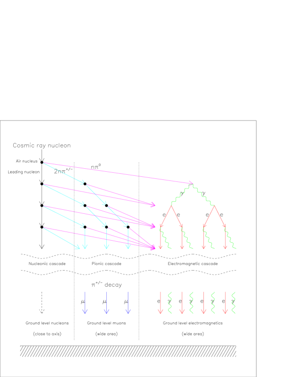
Figure 6: Schematic development of an atmospheric shower. Three components are depicted (case of an hadronic primary).Hadronic cascade (leading nucleon) close to the axis (100m), EM cascade ( $\pi^{0}$ decay) and pion cascade,the last 2 component extend a few km from the axis.

At each step of the cascade the hadronic energy is shared between 70% hadronic and 30% electromagnetic. The shower grows until the average pion energy reaches a critical value ($E_{c}\sim GeV$) where their interaction length is longer than their decay length. At this stage the shower development is at a maximum (about 830$g/cm^{2}$ of atmospheric depth) and starts to very slowly decrease.

Using a very simplified model, as depicted on Figure 7 one can derive the main EAS properties. Let $\lambda~{}$ be the interaction length in Air, $E_{c}~{}$ the critical energy below which particles only decay or loose energy via ionization and $X$ the shower depth in the atmosphere (usually measured in $g/cm^{2}$) then :

• the particle number ($N(X)$) at a given depth $X$ grows like $N_{s}^{X/\lambda}$ (where $N_{s}$ is the number of secondaries in an interaction),

• the secondaries mean energy $E(X)$ at depth $X$ is $E_{0}/N(X)$

• and since by definition $E_{c}=E_{0}/N(X_{max})=E_{0}/N_{max}$ one can show that the position of the shower maximum $X_{max}$ varies like $\lambda~{}log(E_{0})$ while the size at maximum $N_{max}$ is proportionnal to the primary energy.

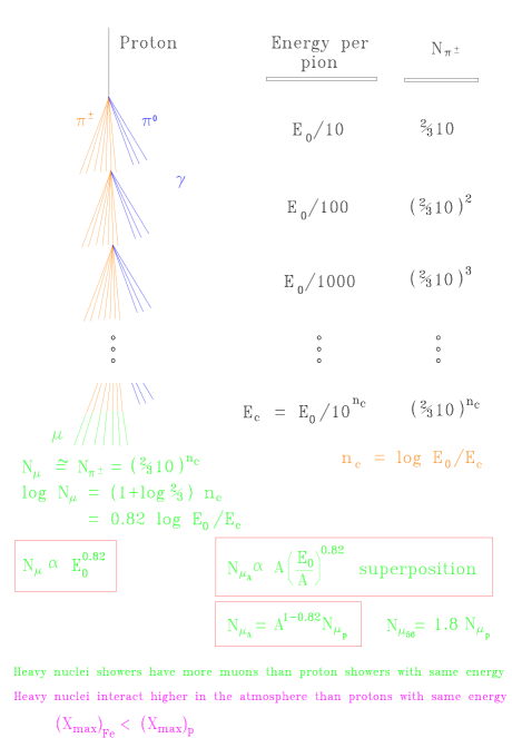
Figure 7: A simplified shower development model.

At ground level most of the energy is caried out by photon and electrons and their number is proportionnal to the total shower energy, i.e. to the primary cosmic ray energy.

$$E_{EM}\propto(N_{\gamma}+N_{e^{+}e^{-}})<\epsilon>\quad\propto E_{prim}$$

where $<\epsilon>$ is the mean photon or electron/positron energy at ground level ($\sim 10MeV$).

The muon content of the shower does not scale linearly with energy. Muons are mainly produced through pion decay whose energy increases faster ($\propto E_{prim}$) than their number ($\propto\log{E_{prim}}$) therefore the number of pions reaching the critical energy and decaying into muons is not proportionnal to the primary energy. With a simple Monte Carlo one can show that for a proton primary the muon number scale as :

$$N_{\mu}^{p}(E)\propto E^{0.85}.$$

For nuclei, the superposition principle stipulates that a nucleus ${}^{A}N$ of total energy $E_{0}$ is equivalent to $A$ proton of energy $E_{0}/A$. Therefore the muon content of an EAS initiated by a nucleus will contain more muons than the EAS initiated by a single proton of the same energy :

$$N_{\mu}^{A}(E)\propto A^{0.15}\times N_{\mu}^{p}(E).$$

Therefore an Iron primary (${}^{56}Fe$) gives 80% more muons then a proton of the same energy.

For lighter primaries such as photons, the muon component will be much smaller as the number of pion produced in the cascade is greatly reduced. The position of the shower maximum will also strongly depends on the primary type (photon or neutrinos) and on additionnal phenomena such as conversion in the geomagnetic field and the Landau Pomeranchuk Migdal effect[30]. This effect describes the decrease of the photon/electron nucleus cross-sections with energy and with the density of the medium with which they interact.

Let’s conclude by stressing that the experimental measurements of both the EAS muon content and maximum depth in the atmosphere are of the outmost importance to derive informations about the primary cosmic ray nature.

3.2 Spatial structure

An EAS is essentially a thin disk (a few $\mu s$ thickness) of particles moving at the speed of light. The longitudinal and the lateral development as well as the time structure of the shower are characteristics of its nature. In the following we’ll describe the dominant features of those profiles.

As was previously mentionned, the longitudinal development is characterized by a maximum reached at an atmospheric depth of 830 g/cm² (or an equivalent altitude of about 1800 meters for vertical showers). At maximum, the shower contains about $7\times 10^{9}$ electrons. The depth of maximum is a function of the primary energy and type,

$$X_{max}(10\times E_{0})=X_{max}(E_{0})+55~{}(g/cm^{2})$$

and, from the superposition principle,

$$X_{max}(^{56}F_{e};E_{0})=X_{max}(p;E_{0})-100~{}(g/cm^{2})$$

The electrons contained in the shower excite the Nitrogen molecules of the atmosphere which produce fluorescence light. As the emision of light is proportionnal to the number of ionizing particles, the fluorescence light follows the longitudinal developmewnt of the shower. Such a profile as measured by the Fly’s Eye optical device is shown on Figure 8.

Figure 8: A longitudinal profile as measure by the Fly’s Eye experiment. The measured energy is $3\times$10²⁰ eV.

The lateral development of the shower is represented by its Molière radius (or the distance within which 90% of the total energy of the shower is contained) which, in “standard air” is 70 m. However, the actual extension of the shower at ground level is of course much larger. As an example, at a distance of 1 km from the shower axis, the average densities of photons/electrons/muons are 30/2/1 per m² respectively.

The particle density as a function of distance to the shower axis is parameterized by the “lateral distribution function” :

$$\rho(r)\propto k\times r^{-[\eta+f(r)]}$$

where $f$ and $k$ depend on the ground detector type and $\eta$ upon the primary incident angle and energy. For $r>800m$ this (empirical) expression must be modified by a factor $(r/800)^{1.03}$ to better modelize the experimental data. Patricle densities are presented on figure 9 as well as the corresponding response of water Cherenkov detector.

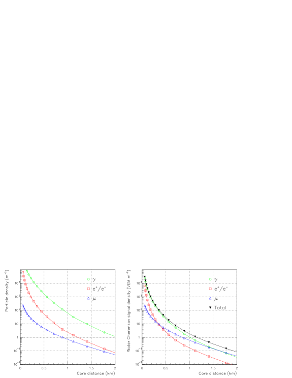
Figure 9: Particle densities as a function of core distance (left). Corresponding detector response for a water Cherenkov tank (right).

The particle arrival time at a given detector is essentially driven by geometrical arguments. Defining the shower plane as the plane tangent to the shower front and perpendicular to its axis one observes that far from the core particles arrive after the shower plane. In fact the shape of the shower front above the shower plane can be modeled with a cone.

• At a distance R from the core particles are spread over a time interval which is roughly proportionnal to R. Moreover, this time spread increases when $X_{max}$ increases.

• Muons, as they can travel quite far and almost straight, arrive in general earlier than the electromagnetic component.

The first item allows to distinguish small close-by showers from far away large ones while the second allows to count muons without a particle identification detector. As an example a ${}^{56}Fe$ primary gives more muons and interacts sonner (higher) in the atmosphere. Consequently, the signal rise time (for a signal proportionnal to the particle number) will be slower than for a proton shower.

Let $t_{\alpha}$ be the time for which $E(t_{\alpha})=\alpha\times E(+\infty)$ with $\alpha\in[0,1].$ $E(t)$ is the integrated detector signal amplitude as a function of time. Then $t_{\alpha-\beta}=t_{\beta}-t_{\alpha}$ is an indirect measure of $X_{max}$ i.e. of the primary type.

Fluctuations :
All the above distributions are subject to fluctuations in the ground particle distibutions. Those fluctuations depend only weakly on the depth and characteristics of the first interaction. There is an optimal distance from the shower core where one can estimate the primary energy from the ground particle density. The shower to shower “physical” fluctuations due to the variation in the first interaction important near the core decrease with distance, while the statistical fluctuation in the densities increase.

3.3 Monte Carlo descriptions

All these effects are studied through heavy use of EAS Monte Carlo programs such as AIRES,[31] CORSIKA,[32] HEMAS[33] or MOCCA.[34] At the UHECR ranges, where the center-of-mass energies are much higher (almost two orders of magnitude) than those attainable in the future accelerator (like LHC), the correct modelling of the EAS in these programs becomes delicate.

Some data are available from accelerator experiments such as HERA,[35] and showers of about $10^{16}$ eV are now being well studied through experiments such as KASCADE.[36] The models are thus constrained at lower energies and then extrapolated at higher ones.

The most commonly used models for the high energy hadronic interactions are SIBYLL,[37] VENUS,[38] QGSJet[39] and DPMJet.[40] Interactions at lower energies are either processed through internal routines of the EAS simulation programs or by well-known packages such as GHEISHA.[41] Some detailed studies of the different models are available.[42] The main shower parameters, such as the reconstructed direction and energy of the primary CR, are never strongly dependent on the chosen model. However, the identification of the primary is more problematic. Whatever technique is chosen, the parameters used to identify the primary cosmic ray undergo large physical fluctuations which make an unambiguous identification difficult.

A complete analysis done by the KASCADE group on the hadronic core of EAS[36] has put some constraints on interaction models beyond accelerator energies. Various studies seem to indicate QGSJet as being the model which best reproduces the data[42, Erlykin] with still some disagreement at the knee energies ($10^{16}$ eV). For the highest energies, additionnal work (and data) is needed to improve the agreement between the available models.

4 Detection techniques

When the cosmic ray flux becomes smaller than 1 particle per m² per year, satellite borne detectors are not appropriate any more. This happens above $10^{16}$ eV (the so-called “knee” region). Then large surfaces are needed and the detectors become ground-based. What they detect is not the incident particle itself but the Extensive Air shower described in the previous section.

All experiment aim to measure as accuratly as possible the three following quantities  :

• The primary direction (given by the shower axis),

• the primary energy,

• the primary nature (or mass).

There are two major techniques used. The first, and the most frequent, is to build an array of sensors (scintillators, water Cerenkov tanks, muon detectors) spread over a large area. The detectors count the particle densities sampling the EAS particles hitting the ground. The surface of the array is chosen in adequation with the incident flux and the energy range one wants to explore. From the timed sampling of the lateral development of the shower at a given atmospheric depth one can deduce the direction, the energy and possibly the identity of the primary CR. The second technique, until recently the exclusivity of a group from the University of Utah, consists in studying the longitudinal development of the EAS by detecting the fluorescence light produced by the interactions of the charged secondaries.

4.1 The optical fluorescence technique

The basic principle is simple[43] the fluorescence light which is quickly and isotropically emitted by the nitrogen atoms of the atmosphere can be detected by a photo-multiplier. The emission efficiency (ratio of the energy emitted as fluorescence light to the deposited one) is poor, less than 1%, therefore observations can only be done on clear moonless nights (which results in an average 10% duty cycle) and low energy showers can hardly be observed. However, at higher energies, the huge number of particles in the shower  produce enough light to be detected even at large distances.

The fluorescence yield is 4 photons per electron per meter at ground level pressure. The emitted light is typically in the 300-400 nm UV range to which the atmosphere is quite transparent. Under favorable atmospheric conditions an UHECR shower can be detected at distances as large as 20 km, about two attenuation lengths in a standard desert atmosphere at ground level.

The first successful detectors based on these ideas were built by a group of the University of Utah, under the name of “Fly’s Eyes”[44], and used with the Volcano Ranch ground array[45]. A complete detector was then installed at Dugway (Utah) and started to take data in 1982. An updated version, the High-Resolution Fly’s Eye, or HiRes[46], is presently running on this same site.

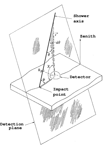
Figure 10: The principle of the detection of an EAS by a fluorescence telescope.

Figure 10 shows the geometry of the detection of an air shower by a Fly’s Eye type detectors. The detector sees the shower as a variable light bulb  moving at the speed of light along the shower axis. The detector itself is a set of phototubes mounted on a “camera” set at the focal plane of a mirror. Each phototube sees a small portion of the sky (typically $1^{\circ}$ squared). A fit of the hit tubes pattern determines with a precision better than one degree the plane containing the detector and the shower axis. In the stereo mode (EAS seen by two telescopes installed a few km apart), two planes are thus reconstructed and their intersection gives the incident direction with good precision. In the mono mode (EAS seen by a single telescope), one relies on the time of arrival of the photons on the tubes. A good reconstruction of the direction (the $\Psi$ angle) then needs a larger number of pixels, enough to measure simultaneously the angular velocity and the angular acceleration of the shower development. Finally, in the hybrid mode, i.e. simultaneous detection of the EAS with a fluorescence telescope and a ground array, the position of the core given by the array determines the final geometry. For 100 EeV showers, a precision of $0.2^{\circ}$ can then be reached.

The fluorescence technique is the most appropriate way to measure the energy of the incident cosmic ray: it is a partial calorimetric measurement with continuous longitudinal sampling. The amount of fluorescence light emitted is proportional to the number of charged particles in the shower. The EAS has a longitudinal development usually parameterized by the analytic Gaisser-Hillas function giving the size $N_{\mbox{e}}$ of the shower (actually the number of the ionizing electrons) as a function of atmospheric depth $x$:

$$N_{\mbox{e}}(x)=N_{\mbox{max}}\left(\frac{x-x_{0}}{X_{\mbox{max}}-x_{0}}\right)^{(X_{\mbox{max}}-x_{0})/\lambda}\mbox{e}^{(X_{\mbox{max}}-x)/\lambda}$$

where $\lambda=70\,$g/cm², $x_{0}$ is the depth at which the first interaction occurs, and $X_{\mbox{max}}$ the position of the shower maximum. The total energy of the shower is proportional to the integral of this function, knowing that the average energy loss per particle is 2.2 MeV/g cm^-2.

In practice several effects have to be taken into account to properly convert the detected fluorescence signal into the primary energy. These include the subtraction of the direct or diffused Cerenkov light, the effects of Rayleigh and Mie scatterings, the dependence of the attenuation on altitude (and elevation for a given altitude) and atmospheric conditions, the energy transported by the neutral particles (neutrinos), the hadrons interacting with nuclei (whose energy is not converted into fluorescence) and penetrating muons whose energy is mostly dumped into the earth. One also has to take into account that a shower is never seen in its totality by a fluorescence telescope: the Gaisser-Hillas function parameters are measured by a fit to the visible part of the shower, (there is usually a missing part at the beginning, close to the interaction point, and at the end, tail absorbed by the earth). All these effects contribute to the systematic errors in the energy measurement which needs sophisticated monitoring and calibration techniques. The overall energy resolution one can reach with a fluorescence telescope is of course dependent on the EAS energy but also on the detection mode (mono, stereo or hybrid). The HiRes detector should have a resolution of 25% or better above 30 EeV in the mono mode. This improves significantly in the stereo or hybrid modes (about 3% median relative error at the same energy in the latter case).

The identification of the primary cosmic ray with a fluorescence telescope is based on the shower maximum position in the atmosphere ($X_{\mbox{max}}$). Simulations show typical values of 750 and 850 g/cm² for iron nuclei and protons respectively. Unfortunately, the physical fluctuations of the first interaction point and of the shower development (larger than the measurements precision) blur this ideal image. Therefore, one must look for statistical means of studying the chemical composition and/or use the hybrid detection method where a multi-variable analysis becomes possible.

The former method uses the so-called elongation rate measured for a sample of showers within some energy range. The depth of the shower maximum as a function of the energy for a given composition is given by[47]:

$$X_{\mbox{max}}=D_{\mbox{el}}\ln\left(\frac{E}{E_{0}}\right)$$

where $E_{0}$ is a parameter depending on the primary nucleus mass. Therefore, incident samples of pure composition will be displayed as parallel straight lines with the same slope $D_{\mbox{el}}$ (the elongation rate) on a semi-logarithmic diagram.

4.2 The ground array technique

The surface of the array is a direct function of the expected incident flux and of the statistics needed to answer the questions at stake. The 100 km² AGASA[Yoshoda, 53] array is appropriate to confirm the existence of the UHECR with energies in excess of 100 EeV (which it detects at a rate of about one event per year). To explore the properties of these cosmic rays and hopefully answer the open question of their origin, the Auger Observatory with its 6000 km² surface over two sites will be very helpfull.

The array detectors count the number of secondary particles which cross them as a function of time, sampling the non-absorbed part of the shower which reaches the ground. The incident cosmic ray direction and energy are measured by assuming that the shower has an axial symmetry. This assumption is valid for not too large zenith angles (usually $\theta<60^{\circ}$). At larger angles the low energy secondaries are deflected by the geomagnetic fields and the analysis becomes more delicate.

The direction of the shower axis (hence of the incident primary) is reconstructed by fitting the “lateral distribution function” (LDF) to the measured densities. The LDF explicit form depends on each experiment. The Haverah Park experiment[48] (an array of water-Cerenkov tanks) used the function:

$$\rho(r,\theta,E)=kr^{-[\eta(\theta,E)+r/4000]}$$

as the LDF for distances less than 1 km from the shower core. Here $r$ is in meters, and $\eta$ can be expressed as:

$$\eta(\theta,E)=a+b\sec\theta+c\log(E/E_{0})$$

with appropriate values for all the parameters taken from shower theory and Monte Carlo studies in a given energy range. At larger distances (and higher energies), this function has to be modified to take into account a change in the rate at which the densities decrease with distance. A much more complicated form is used by the AGASA group.[49] However, the principle remains the same.

Once the zenith angle correction is made for the LDF, an estimator of the primary energy is extracted from this function. At energies below 10 EeV, the optimal estimation distance is 600 m from the shower core, a value slowly increasing with energy, reaching 1000m in the UHECR range. Once this value is determined, the primary energy is related to it by a quasi-linear relation:

$$E=k\rho_{optimal}^{\alpha}$$

where $\alpha$ is a parameter close to 1. Of course, to be able to reconstruct the LDF, many array stations have to be hit at the same time. The spacing between the stations determines the threshold energy for a vertical shower: the 500 m spacing of the Haverah Park triggering stations corresponds to a threshold of a few $10^{16}$ eV, while the 1.5 km separation of the Auger Observatory stations gives almost 100% efficiency above 10 EeV.

In a ground array, the primary cosmic ray’s identity is reflected in the proportion of muons among the secondaries at ground level. Here a proper estimator is therefore the ratio of muons to electrons - and eventually photons, if they are detected -. When a ground array has muon detecting capabilities (water Cerenkov tanks, buried muon detectors), one measures directly the muon to electron ratio. Otherwise, an indirect method is given by the signal rise time.

5 Experimental results

It is outside the scope of this lecture to present the full history of the cosmic ray detection and studies. This would cover the whole century (1912 is the year of the first decisive balloon experiments by Victor Hess). As a starting point for the genesis of the UHECR physics, one can use the first observations of Pierre Auger and collaborators[50] done in 1938. They studied the coincidence rates between counters with increasing separation (up to 150 m in their first experiments in Paris, more than 300 m when they repeated them at the Jungfraujoch in Switzerland). They inferred from these very modest measurements the existence of primary cosmic rays with energies as large as 1 PeV (10¹⁵ eV).

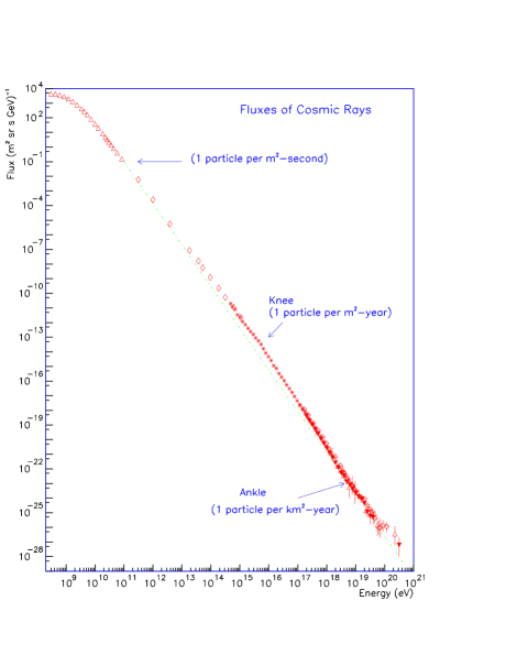
Figure 11: The all-particle spectrum of cosmic rays

Figure 11 is a compilation[51] of the differential spectrum of cosmic ray flux as a function of energy. On this figure, integrated fluxes above three energy values are also indicated: 1 particle/m²-second above 1 TeV, 1 particle/m²-year above 10 PeV, 1 particle/km²-year above 10 EeV. Ground detectors are the only alternative for the highest energy part of the spectrum.

In this section, and unless otherwise specified, we shall pay special attention to the events with energies exceeding 100 EeV. This value has no particular physical meaning except that it is well above the GZK cutoff.

5.1 The energy spectrum and flux

The energy spectrum (Figure 11) ranges over 13 orders of magnitude in energy and 34 orders of magnitude in flux. However, if one discards the saturation region at the lowest energies, the spectrum is surprisingly regular in shape. From the GeV energies to the GZK cutoff, it can be represented simply by three power-law curves interrupted by two breaks, the so-called “knee” and “ankle”.

file=./agasa.eps,width=270pt

Figure 12: Energy spectrum above 100 PeV. The compilation is from Ref. updated by M.Nagano (private communication).

The flux of supra-GZK events is extremely low. Figure 12 is a zoom on the highest energy part of the total spectrum. On this figure, the energy spectrum is multiplied by $E^{3}$ so that the part below the EeV energies becomes flat. One can see the ‘ankle’ structure in its complexity: a steepening around the EeV and then a confused region where the GZK cutoff is expected. The ultimate data points come from very few events hence their large error bars. Due to normalization problems it is difficult to compare different experiments. On Figure 13 where the AGASA data alone are displayed,[53] one has a clearer view of what can be expected from a cosmological distribution of conventional sources and what is observed.

file=./takeda.ps,bbllx=117pt,bblly=228pt,bburx=512pt,bbury=602pt,width=8cm,clip=

Figure 13: Highest energy region of the cosmic ray spectrum as observed by the AGASA detector The figures near the data points indicate the number of events in the corresponding energy bin. The arrows show 90% confidence level upper limits. The dashed line is the expected spectrum if the sources were cosmologically distributed.

The GZK cutoff is clearly visible on the dashed line while the data suggests a change of slope as if a new phenomenon was rising above a steeply falling spectrum. The cutoff, that would be expected if the sources were cosmologically distributed and if the observed cosmic rays had no exotic propagation or interaction properties, is not present in the observed data.

The flux of the highest energy cosmic rays cannot be deduced from the data above the cutoff energies: no reliable fit to the spectrum shape is feasible in this region. A reasonable estimate can be ontained taking the ratio of the total experimental exposure to the number of events observed. The exposure to events above the GZK cutoff for AGASA, Fly’s Eye and Haverah Park detectors together, is of the order of 2000 km² sr yr. The number of events observed in this energy range yields an integrated flux which can be parameterized by:

$$I(E>E_{0})\approx\left(\frac{E_{0}}{10\,\mbox{EeV}}\right)^{-2}\,\mbox{km}^{-2}\mbox{sr}^{-1}\mbox{year}^{-1}$$ (10)

With $E_{0}=100$ EeV. Therefore the expected flux above 100 EeV is (only) 1 particle per km² per century.

5.2 The chemical composition

The UHECR chemical composition is very likely to be unveiled only on a statistical basis. What we know at present is weak and controversial due to the limited number of events observed. The most recent information comes from the Fly’s Eye and AGASA experiments. The Fly’s Eye studies[44] (between 0.1 EeV and 10 EeV) are based on $X_{\mbox{max}}$ behavior as a function of the logarithm of the primary energy. With this method, their data show evidence of a shift from a dominantly heavy composition (compatible with iron nuclei) to a light composition (protons). In this framework UHECR are mainly protons.

The AGASA group based their primary identification on the muon content of the EAS at ground level,[54]. Initially the conclusion of the AGASA experiment was quite opposite to the Fly’s Eye: no change in chemical composition. However a recent critical review of both methods[55] showed that the inconsistencies were mainly due to the scaling assumption of the interaction model used by the AGASA group. The authors concluded that if a model with a higher (compared to the one given by scaling) rate of energy dissipation at high energy is assumed, as indicated by the direct $X_{\mbox{max}}$ measurements of the Fly’s Eye, both data sets demonstrate a change of composition, a shift from heavy (iron) at 0.1 EeV to light (proton) at 10 EeV. Different interaction models as long as they go beyond scaling in their energy dissipation, would lead to the same qualitative result but possibly with a different rate of change.

Gamma rays have also high cross sections with air and are still another possible candidate for UHECR but no evidence were found up to now for a gamma signature among the Big Events. The most energetic Fly’s Eye event was studied in detail[56] and found incompatible with an electromagnetic shower. Both interpretations of the AGASA and the Fly’s Eye data favor a hadronic origin.

5.3 Distribution of the sources

A necessary ingredient in the search for the origin of the UHECR is to locate their sources. This is done by reconstructing the incident cosmic ray’s direction and checking if the data show images of point sources or correlations with distributions of astrophysical objects in our vicinity. In the following we will consider the effects of the galactic and extragalactic magnetic fields on protons and we will show that for supra-GZK energies, proton astronomy is possible to some extent. We will then give a review of what we can extract from the present data.

5.3.1 Magnetic fields

There are a limited number of methods to study the magnetic fields on galactic or extragalactic scales.[57] One is the measure of the Zeeman splitting of radio or maser lines in the interstellar gas. This method informs us mainly on the galactic magnetic fields, as extragalactic signals suffer Doppler smearing while the field values are at least three orders of magnitude below the galactic ones. The magnetic field structure of the galactic disc is therefore thought to be rather well understood. One of the parameterizations currently used is that of Vallée[58]: concentric field lines with a few $\mu$G strength and a field reversal at about one half of the disk radius. Outside the disk and in the halo, the field model is based on theoretical prejudice and represented by rapidly decreasing functions (e.g. gaussian tails).

The study of extragalactic fields is mainly based on the Faraday rotation measure (FRM) of the linearly polarized radio sources. The rotation angle is a measurement of the integral of $n_{e}B_{\parallel}$ along the line of sight, where $n_{e}$ is the electron/positron density and $B_{\parallel}$ the longitudinal field component. Therefore, the FRM needs to be complemented by the measurement of $n_{e}$. This is done by observing the relative time delay versus frequency of waves emitted by a pulsar. Since the group velocity of the signal depends simultaneously on its frequency but also on the plasma frequency of the propagation medium, measurement of the dispersion of the observed signals gives an upper limit on the average density of electrons in the line of sight. Here again, because of the faintness of extragalactic signals, our knowledge of the strength and coherence distances of large scale extragalactic fields is quite weak and only upper limits over large distances can be extracted. An educated guess gives an upper limit of 1 nG for the field strength and coherence lengths of the order of 1 Mpc.[57]

file=./angular.eps,height=214pt,width=322pt

Figure 14: Effect of magnetic fields on the propagation of a proton as a function of energy: angular deviation (left) and time delay (right), with respect to a straight line trajectory, in the framework of three realistic scenarios (see text).

A few other more or less indirect methods exist for the study of large scale magnetic fields. If the UHECR are protons and if they come from point-like sources, the shape of the source image as a function of the cosmic ray energy will certainly be one of the most powerful of them. The Larmor radius $R$ of a charged particle of charge $Ze$ in kiloparsecs is given by:

$$R_{\mbox{kpc}}\approx\frac{1}{Z}\left(\frac{E}{1\,\mbox{EeV}}\right)\left(\frac{B}{1\,\mu\mbox{G}}\right)^{-1}$$

The Larmor radius of a charged particle at 320 EeV is larger than the size of the galaxy if its charge is less than 8. If we take the currently accepted upper limit ($10^{-9}$ G) for the extragalactic magnetic fields, a proton of the same energy should have a Larmor radius of 300 Mpc or more.

In Figure 14, three different situations are envisaged to evaluate the effects of magnetic fields on a high energy cosmic proton. The situations correspond to what is expected a-) for a trajectory through our galactic disk (0.5 kpc distance inside a 2 $\mu$G field) or b-) over a short distance (1 Mpc) through the extragalactic (1 nG) field (same curve), and finally c-) a 30 Mpc trajectory through extragalactic fields with a 1 Mpc coherence length (multiple scattering effect). One can see that at 100 EeV, the deviation in the third case would be about $2^{\circ}$. This gives an idea of the image size if the source is situated inside our local cluster or super-cluster of galaxies. Since the angular resolution of the (present and future) cosmic ray detectors can be comparable to or much better than this value, we expect to be able to locate point-like sources or establish correlations with large-scale structures.

However, let us remember that this working hypothesis of very weak extragalactic magnetic fields is not universally accepted. Several authors recently advocated our bad knowledge of those fields arguing for stronger magnetic fields (typically at the $\mu$G level) either locally[60] or distributed over larger, cosmological, scales.[61]

5.3.2 Anisotropies

file=./bigevents.eps,bbllx=79pt,bblly=417pt,bburx=528pt,bbury=627pt,width=12cm,clip=

Figure 15: Arrival directions of cosmic rays with energies above 10 EeV (equatorial coordinates), as measured by the AGASA experiment. The thick dotted lines show the galactic and supergalactic planes (GC indicating the galactic center). The shaded regions are those invisible to the AGASA detector. See text.

In the search for potential sources, the propagation arguments incite us to look for correlations with the distribution of astrophysical matter within a few tens of Mpc. In our neighborhood, there are two structures showing an accumulation of objects, both only partially visible from any hemisphere: the galactic disk on a small scale and the supergalactic plane on a large scale, a structure roughly normal to the galactic plane, extending to distances up to $z\approx 0.02$ (about 100 Mpc).

In equatorial coordinates isotropically distributed sources, give a uniform right ascension distribution of events and a declination distribution which can be parameterized with the known zenith angle dependence of the detector aperture.

The most recent analysis on the correlation between arrival directions and possible source locations was done by the AGASA experiment for the highest energy range.[62] The analysis is based on 581 events above 10 EeV, a subset of 47 events above 40 EeV and 7 above 100 EeV. Figure 15 is a compilation of the total sample in equatorial coordinates. The dots, circles and squares are respectively events with energies above 10, 40 and 100 EeV. The data show no deviation from the expected uniform right ascension distribution. An excess of 2.5 $\sigma$ is found at a declination of $35^{\circ}$ and can be interpreted as a result of observed clusters of events (see below). No convincing deviation from isotropy is found when the analysis is performed in galactic coordinates.

The same collaboration[63] made also a similar analysis for the lower energy region (events down to 1 EeV and detected with zenith angles up to $60^{\circ}$). In this article, a slight effect of excess events in the direction of the galactic center was announced. A similar study[64] with the Fly’s Eye data, concludes on a small correlation with the galactic plane for events with energies lower than 3.2 EeV and isotropy for higher energies.

In summary, both the AGASA and Fly’s Eye experiments seem to converge on some anisotropy in the EeV range (correlation with the galactic plane and center) and isotropy above a few tens of EeV. This result may seem surprising - one naively expects the correlations to be stronger when the cosmic rays have large magnetic rigidity. It is actually explained by the fact that the low energy component may be dominantly galactic heavy nuclei (see the section on chemical composition), hence a (weak) correlation with the galactic plane, whereas the higher energy cosmic rays would be dominated by extragalactic protons.

5.4 Point sources?

If the sources of UHECR are nearby astrophysical objects and if, as expected, they are in small numbers, a selection of the events with the largest magnetic rigidity would combine into multiplets or clusters which would indicate the direction to look for an optical or radio counterpart. Such an analysis was done systematically by the AGASA group.[62]

file=./bigevents.eps,bbllx=71pt,bblly=187pt,bburx=528pt,bbury=398pt,width=12cm,clip=

Figure 16: Arrival directions of cosmic rays with energies above 40 EeV (galactic coordinates), as measured by the AGASA experiment.See text.

Figure 16 shows the subsample of events in the AGASA catalog with energies in excess of 100 EeV (squares) and in the range 40-100 EeV (circles). A multiplet is defined as a group of events whose error boxes ($2.5^{\circ}$ circles) overlap. One can see that there are three doublets and one triplet. If one adds the Haverah Park events, the most southern doublet also becomes a triplet. The chance probability of having as many multiplets as observed with a uniform distribution are estimated by the authors to less than 1%.

A search for nearby astrophysical objects within an angle of $4^{\circ}$ from any event in a multiplet was also done, and produced a few objects. One of the most interesting candidates is Mrk 40, a galaxy collision, since the shock waves generated in such phenomena are considered by some authors[65] as being valid accelerating sites.

Another way of using the observed multiplets, assuming that they come from an extragalactic point source, is to consider the galactic disk as a magnetic spectrometer which can give information on the charge of the incident cosmic rays. Cronin[66] made such an analysis on the doublet where the energy difference between the two events is the largest (a factor of four). He uses the magnetic field model of Vallée[58] to trace back the detected couple of events outside of the galaxy assuming various charges. It is shown that the maximum charge compatible with a separation less than the detector’s angular resolution is 2 for the members of the doublet with conservative integrated values for the magnetic field, a result compatible with UHECR being mostly protons.

6 Conclusions

The UHECR were a puzzle when they were first observed, more than 30 years ago. They still are. Among all the tentative explanations given to their existence none fully explains the whole set of observation.

The past experiments which explored this field could do hardly better than convince us of the existence of the UHECR above the GZK cutoff. Statistics which should make us able to locate the sources, reconstruct the shape of the cosmic ray spectrum above the cutoff and study the chemical composition will soon be provided by the ongoing (HiRes, AGASA) and oncoming (Auger, Telescope-Array, OWL/Airwatch, EUSO) experiments.

The references given as astro-ph/xxxxxxx or hep-ph/xxxxxxx are articles available from the Web electronic preprint archive at the URL http://xxx.lanl.gov/

References

- [1] K. Greisen, Phys. Rev. Lett. 16 (1966) 748. G.T.Zatsepin, V.A.Kuzmin, JETP Lett. 4 (1966) 78.
- [2] P. Bhattacharjee, G. Sigl, “Origin and propagation of extremely high energy cosmic rays”, astro-ph/9811011, to be published in Physics Reports.
- [3] I. F. M. Albuquerque, G. R. Farrar, E. W. Kolb, Phys.Rev. D59 (1999).
- [4] A. Karle et al, Phys. Rev. Lett. B347 (1995) 161.
- [5] G. Sigl, M. Lemoine, P. Biermann, Astropart. Phys. 10 (1999) 141.
- [6] A. Venkatesan, M. Coleman Miller, A. V. Olinto, Ap. J. 484 (1997) 323.
- [7] R. J. Protheroe “Origin and propagation of the highest energy cosmic rays”, Towards the Millennium in Astrophysics: Problems and Prospects, Erice 1996, (World Scientific, Singapore).
- [8] L. O’C. Drury, Rep. Prog. Phys. 46 (1983) 973.
- [9] J. G. Kirk and P. Duffy, “Particle acceleration and relativistic shocks”, astro-ph/9905069.
- [10] A. M. Hillas, Annual Review Astron. Astrophys. 22 (1984) 425.
- [11] P. L. Biermann, Phys. Rev. D51 (1995) 3450.
- [12] F. Halzen, E. Zas, Ap. J. 488 (1997) 669.
- [13] E. Waxman, “Gamma-Ray Burts, Cosmic-Rays and Neutrinos”, Nuclear Physics B, Proceedings Supplements, Volume 87, July 2000.
- [14] G. R. Farrar, P. L. Biermann, Phys. Rev. Lett. 81 (1998) 3579.
- [15] B. Andersson et al. Phys. Rep. 97 (1983) 31.
- [16] Y. I. Azimov et al. Z. Phys. C 27 (1985) 65.
- [17] A. Vilenkin, E. P. S. Shellard, “Strings and Other Topological Defects”, Cambridge Univ. Press, Cambridge, 1994.
- [18] T. Vachaspati, “Formation of Topological Defetcs”, ICTP summer school on Cosmology (1997), hep-ph/9710292.
- [19] T. Vachaspati, “Formation, Interaction and Observation of Topological Defects”, Les Houches (1998), astro-ph/9903362.
- [20] P. Bhattacharjee, “Ultrahigh Energy Cosmic Rays from Topological Defects — Cosmic Strings, Monopoles, Necklaces, and All That”, astro-ph/9803029.
- [21] V. Berezinsky, P. Blasi, A. Vilenkin, Phys. Rev. D58 (1998), 103515.
- [22] Ya. Zel’dovich, I. Kobzarev, L. Okun, Zh. Eksp. Teor. Fiz. 67 (1974) 3.
- [23] A. H. Guth, Phys. Rev. D23 (1981) 347.
- [24] R. H. Brandenberger, Pramana 51 (1998) 191. See also hep-ph/9806473.
- [25] C. T. Hill, Nucl. Phys. B 224 (1983) 469.
- [26] D. N. Schramm, C. T. Hill, Proc. 18th ICRC (1983) 393.
- [27] P. Bhattacharjee, C. T. Hill, D. N. Schramm, Phys. Rev. Lett. 69 (1992) 567.
- [28] V. Berezinsky, ‘‘Ultra High Energy Cosmic Rays’’, hep-ph/9802351
-
[29]
S. C. Corbato et al, Proc. of the International Workshop
on Techniques to Study Cosmic Rays with Energies Greater than eV,
Paris, Nucl. Phys. B (Proc. Suppl.) 28B (1992) 36.
Web site: sunshine.chpc.utah.edu/research/cosmic/hires/ -
[30]
L. Landau, I. Pomeranchuk, Dokl. Akad. Nauk. SSR 92 (1953) 535.
A. B. Migdal, Phys. Rev. 103 (1956) 1811. - [31] S. J. Sciutto, “Air Shower Simulations with the AIRES System”, astro-ph/9905185.
-
[32]
J. N. Capdevielle et al, Kernforschungszentrum
Karlsruhe preprint KfK 4998 (1992).
J. Knapp, D. Heck, preprint KfK 5196 (1993). - [33] Web site: osf1.lngs.infn.it/~carboni/Hemas/doc/
- [34] A. M. Hillas, Proc. 19th ICRC (La Jolla), 1 (1985) 155.
- [35] R. Engel, Xth Int. Symposium on Very High Energy Cosmic Rays Interactions, Gran Sasso (1998).
- [36] H. O. Klages et al (KASCADE Collaboration), Nucl. Phys. B (Proc. Suppl.) 52B (1997) 92.
- [37] R. S. Fletcher et al., Phys. Rev. D50 (1994) 5710.
- [38] K. Werner, Phys. Rep. 232 (1993) 87.
- [39] N. N. Kalmykov, S. S. Ostapchenko, Yad. Fiz. 56 (1993) 105.
- [40] J. Ranft, INFN/AE-97/45, Gran Sasso report, 1997.
- [41] H. Fesefeldt, Report PITHA-85/02 (1985), RWTH Aachen.
-
[42]
J. Knapp, Proc. 25th ICRC, Durban (1997).
T. Antoni et al, “Test of high-energy interaction models using the hadronic core of EAS”, astro-ph/9904287. - [43] G. L. Cassiday, Ann. Rev. Nucl. Part. Sci. 35 (1985) 321. See also Ref.[47], Chapter 6.
- [44] D. J. Bird et al, Ap. J. 424 (1994) 491.
- [45] J. Linsley, Phys. Rev. Lett. 10 (1963) 146.
-
[46]
S. C. Corbato et al, Proc. of the International Workshop
on Techniques to Study Cosmic Rays with Energies Greater than eV,
Paris, Nucl. Phys. B (Proc. Suppl.) 28B (1992) 36.
Web site: sunshine.chpc.utah.edu/research/cosmic/hires/ - [47] For a clear and detailed presentation of EAS properties, see e.g. P. Sokolsky, Introduction to Ultra High Energy Cosmic Ray Physics (Addison Wesley, Frontiers in Physics, 1989), Chapter 3.
- [48] M. A. Lawrence, R. J. O. Reid, A. A. Watson, J. Phys. G. 17 (1991) 773.
- [49] S. Yoshida et al, Astropart. Phys. 3 (1995) 105.
-
[50]
P. Auger, R. Maze, T. Grivet-Meyer, Comptes rendus,
Académie des Sciences 206 (1938) 1721.
P. Auger, R. Maze, Comptes rendus, Académie des Sciences 207 (1938) 228.
P. Auger et al, Rev. Mod. Phys. 11 (1939) 288. - [51] S. Swordy, private communication. The data points are collected from the following experiments: LEAP, Proton, Akeno, AGASA, Fly’s Eye, Haverah Park, Yakutsk.
- [52] For a complete and comprehensive overview of the astrophysical acceleration mechanisms, see M. S. Longair, in High Energy Astrophysics (Cambridge University Press, Cambridge, 2nd edition, 1994), Vol. 2, Chapter 21 and T. K. Gaisser, Cosmic Rays and Particle Physics (Cambridge University Press, Cambridge, 1990), Chapter 11.
-
[53]
M. Takeda et al, Phys. Rev. Lett. 81
(1998) 1163; e-print astro-ph/9807193.
See also: www.icrr.u-tokyo.ac.jp/as/project/agasa.html, the AGASA Web site for regular updates. - [54] N. Hayashida et al, J. Phys. G. 21 (1995) 1101. For recent updates, see also: www.icrr.u-tokyo.ac.jp/as/project/agasa.html.
- [55] B. R. Dawson, R. Meyhandan, K. M. Simpson, Astropart. Phys. 9 (1998) 331.
- [56] F. Halzen et al, Astropart. Phys. 2 (1995) 151.
- [57] P. P. Kronberg, Rep. Prog. Phys. 57 (1994) 325.
- [58] J. P. Vallée, Ap. J. 366 (1991) 450.
- [59] The Pierre Auger Project Design Report, Fermilab, October 1995 (Web site: www.auger.org/admin/).
- [60] M. Lemoine, G. Sigl, P. Biermann, “Supercluster Magnetic Fields and Anisotropy of Cosmic Rays above eV”, astro-ph/9903124.
- [61] G. R. Farrar, T. Piran, “GZK Violation - a Tempest in a (Magnetic) Teapot?”, astro-ph/9906431.
- [62] M. Takeda et al, “Small scale anisotropy of cosmic rays above eV observed with the Akeno Giant Air Shower Array”, astro-ph/9902239.
- [63] N. Hayashida et al, “The anisotropy of cosmic ray arrival directions around eV”, astro-ph/9807045, Astropart. Phys. 10 (1999) 303.
- [64] D. J. Bird et al, “Study of Broad Scale Anisotropy of Cosmic Ray Arrival Directions from eV to eV from Fly’s Eye data”, astro-ph/9806096.
-
[65]
C. Cesarsky, Proc. of the International
Workshop on Techniques to Study Cosmic Rays with Energies Greater than
eV, Paris, Nucl. Phys. B (Proc. Suppl.) 28B (1992) 51.
C. Cesarsky, V. Ptuskin, Proc. 23rd ICRC (Calgary), 2 (1993) 341. - [66] J. W. Cronin, private communication, unpublished.
- [67] R. D. Blanford, “Acceleration of ultra high energy cosmic rays”, e-print astro-ph/9906026 (to be published in Particle Physics and the Universe, Physica Scripta World Scientific.).